


1. Introduction
Currently, our Universe is going through an accelerated period of expansion [1, 2], which is confirmed by supernova research enormous-scale galaxy surveys and cosmic background microwave radiation. The identification of this late-time accelerations source is a crucial cosmic science problem [3]. Several approaches have been proposed for the investigation and understanding of this cosmic acceleration. The modification of the foundational equations of general relativity is one of them [4]. A modified theory of gravity, known as F(R) gravity, modifies the left-hand side of Einstein's field equations for general relativity by adding a function of the scalar curvature, denoted as R. This modification presents a fascinating blend of cosmological and astrophysical implications [5]. F(R) gravity may provide an explanation for the observable universe from the structure formation to the evolution epochs, including radiation/matter dominance, dark energy and inflation [6]. Within the field of gravitational theories, F(R) gravity not only works with both Newtonian and post-Newtonian approximations but also attracts interest as a possible means of explaining the structure formation of the expanding Universe without requiring the mysterious existence of dark matter. Introducing a strange fluid known as dark energy is another fascinating way to understand the accelerated phase of our cosmos. It is the fluid that takes center stage here, exhibiting isotropy and a noticeable negative pressure.
A different narrative is told by the phantom scalar field in which the pressure and energy density both unexpectedly take on negative forms, creating a realistic approximation of the enigmatic dark energy phenomenon. F(R) gravity is interesting because it may be used to explain the fascinating objects in space called black holes. Because of their strong gravitational fields, these mysterious cosmic objects provide a unique lens through which to investigate and test gravitational theories. However, black hole solutions are challenging to obtain from the fourth-order differential equations of F(R) gravity, especially when matter fields are involved. Phantom fields are a further factor to consider as we go through the complexities of F(R) gravity. This setting involves a spin-1 phantom field connected linearly inside a topological metric to the action of F(R) theory. The objective of the investigation is to determine how the phantom field affects the structural and basic characteristics of the resultant solution, adding another level of complexity to the system. As we continue our cosmic exploration, we want to understand the Universe's accelerated dynamics, investigate the mystery of black holes in alternative gravitational theories and explore the fascinating interaction between phantom fields and F(R) gravity. Research on modified gravity theory black holes now functions as an essential framework for quantum gravitational studies and also provides exposure of dark energy regions of space. Einstein gravity established the four laws of black hole mechanics together with SBH = A/4 Bekenstein-Hawking entropy as fundamental principles of classical thermodynamics [7]. The introduction of modified theories, such as F(R), scalar-tensor and Gauss-Bonnet gravities, brought fundamental changes to the thermodynamic behavior because they contain higher-order curvature corrections. The expression of entropy in F(R) gravity contained an ${F}^{{\prime} }(R)$ factor that affects the relation $S\propto {F}^{{\prime} }(R)A$ [8] and has shown deviation from SBH when the spacetime curvatures became very large (such as near singular points or phantom energy domains) [9]. Scalar-tensor theories experienced entropy variability because scalar-field interactions with non-minimal couplings affect both the Hawking temperature and phase-transition behavior [10]. Topological entropy terms evolved from the Euler characteristic in Gauss-Bonnet gravity theories, thus creating variations in P - V criticality behavior of AdS black holes [11].
Generalized entropy formalisms, such as Tsallis, Barrow and Kaniadakis, have become a good way to address most of these challenges. Implementing these approaches, SBH is extended with nonextensive statistics [12], fractal horizons [13] and relativistic kinematics [14], and is consistent with F(R) thermodynamics and the quantum spacetime model. An example is S ∝ A1+∆/2 (where ∆ ∈ [0, 1] is a measure of the fractal structure), which matches the natural algebraic extension of order ∆/2 from F(R)-correction of entropy $S\sim {F}^{{\prime} }(R)A$ when ${F}^{{\prime} }(R)\sim {A}^{{\rm{\Delta }}/2}$ (and takes into account the probability that ${F}^{{\prime} }(R)\sim {A}^{1+{\rm{\Delta }}/2}$ has positive probability) [15]. Generalized entropy is a powerful tool for the study of phantom (A)dS black holes when dark energy effects reinforce thermodynamic instabilities, as in these results [16]. By assuming various modified entropies, authors have discussed the thermodynamic quantities and geometries for various well-known black holes [17-19].
Recently, [4] have developed the phantom (A)dS black hole solutions in F(R) gravity and evaluated various conserved/thermodynamic quantities of the system through the first law of thermodynamics. They also studied the heat capacity and the geometrothermodynamics and suggested useful results in the family of black holes. Here, we investigate the thermodynamic quantities of phantom (A)dS black hole solutions in F(R) gravity by assuming generalized entropy. The paper is arranged as follows. In section 2 , we provide the basic setup of black hole solutions and discuss its horizons. In sections 2 and 3 , thermodynamic properties and geometries are examined. In the last section, we provide our final observations and conclusions.
2. F(R)-gravity-corrected black hole solutions
The action of F(R) gravity coupled to the Maxwell field is given by
$\begin{eqnarray}{I}_{F(R)}={\int }_{\partial M}{{\rm{d}}}^{4}x\sqrt{-g}[F(R)+2{\kappa }^{2}\,\eta \,\unicode{x003DD}],\end{eqnarray}$
where κ2 = 8πG (G is the Newtonian gravitational constant), and g is the determinant of the metric tensor. Moreover, F(R) = R + f(R), where R and f(R) appear as the scalar curvature and arbitrary function of the scalar curvature, respectively. Additionally, the second term is the coupling to the Maxwell field, either a phantom field of spin 1 when η = 1 or when η = -1. However, F = FμνFμν represents the Maxwell invariant, while Fμν appears as the electromagnetic tensor field and its expression is Fμν = ∂uAν - ∂νAμ (Aμ signifies the gauge potential). For simplicity, we assume G = c = 1.The equations of motion for F(R) theory can be obtained by modifying the actions equation (2.1 ) with respect to the gauge field Aμ and the gravitational field gμν. According to this variation, one can get
$\begin{eqnarray}\begin{array}{l}{R}_{\mu \nu }(1+{f}_{{R}_{0}})-\frac{{g}_{\mu \nu }F(R)}{2}+({g}_{\mu \nu }{{\rm{\nabla }}}^{2}-{{\rm{\nabla }}}_{\mu }{{\rm{\nabla }}}_{\nu }){f}_{{R}_{0}}=\,8\pi {T}_{\mu \nu },\\ \quad {\partial }_{\mu }(\sqrt{-g}{F}^{\mu \nu })=0,\end{array}\end{eqnarray}$
where $f(R)=\frac{{\rm{d}}f(R)}{{\rm{d}}R}$ and Tμν is the energy momentum tensor. The description of four-dimensional spacetime can be expressed as follows $\begin{eqnarray}{T}_{\mu \nu }=2\eta \left(\frac{1}{4}{g}_{\mu \nu }\unicode{x003DD}-{F}_{\mu }^{\alpha }{F}_{\mu \alpha }\right).\end{eqnarray}$
Further, we consider a topological four-dimensional static spacetime, which has the following form 2.4 ), g(r) is the metric function and ${\rm{d}}{{\rm{\Omega }}}_{k}^{2}$ is given below
$\begin{eqnarray}{\rm{d}}{s}^{2}=g(r)\,\rm{d}\,{t}^{2}-\frac{{\rm{d}}{r}^{2}}{g(r)}-{r}^{2}{\rm{d}}{{\rm{\Omega }}}_{k}^{2}.\end{eqnarray}$
In the above action, equation ( $\begin{eqnarray}{\rm{d}}{{\rm{\Omega }}}_{k}^{2}=\left\{\begin{array}{ll}{\rm{d}}{\theta }^{2}+{\sin }^{2}\theta {\rm{d}}{\varphi }^{2}, & (k=1)\\ {\rm{d}}{\theta }^{2}+{\rm{d}}{\varphi }^{2}, & (k=0)\\ \,\rm{d}\,{\theta }^{2}+{\sinh }^{2}\theta v{\varphi }^{2}, & (k=-1)\end{array}\right..\end{eqnarray}$
It is important to note that the constant k denotes the possibility of several curvature forms, such as elliptic for k = 1, flat for k = 0 and hyperbolic for k = -1. The authors in [4] have developed the following form of a metric coefficient after solving the field equations of the F(R)-Maxwell (or phantom) model by assuming constant curvature scalar as $\begin{eqnarray}g(r)=k-\frac{2m}{r}+\frac{{R}_{0}{r}^{2}}{12}+\eta \frac{{q}^{2}}{(1+{f}_{{R}_{0}}){r}^{2}},\end{eqnarray}$
here $\begin{eqnarray}{R}_{0}=\frac{2f({R}_{0})}{{f}_{{R}_{0}}-1}.\end{eqnarray}$
The integration constant m is related to the black hole total mass.The Kretschmann scalar is one of the characteristics that can provide light on the existence of a singularity. Using the metric function provided by equation (2.6 ) to examine the four-dimensional spacetime given by equation (2.4 ), we can derive the Kretschmann scalar as follows [4]
$\begin{eqnarray}{R}_{\alpha \beta \gamma \delta }{R}^{\alpha \beta \gamma \delta }=\frac{{R}_{0}^{2}}{6}+\frac{48{r}^{2}}{{r}^{6}}-\frac{96m\eta {q}^{2}}{(1+{f}_{{R}_{0}}){r}^{7}}+\frac{56{\eta }^{2}{q}^{4}}{{(1+{f}_{{R}_{0}})}^{2}{r}^{8}},\end{eqnarray}$
which leads to $\begin{eqnarray}\mathop{\mathrm{lim}}\limits_{r\to 0}\,{R}_{\alpha \beta \gamma \delta }{R}^{\alpha \beta \gamma \delta }\longrightarrow \infty ,\end{eqnarray}$
as r approaches zero. At r = 0, a curvature singularity exists, whereas at r ≠ 0, it remains finite. The Kretschmann scalar exhibits asymptotic behavior, as described below $\begin{eqnarray}\mathop{\mathrm{lim}}\limits_{r\to 0}\,{R}_{\alpha \beta \gamma \delta }{R}^{\alpha \beta \gamma \delta }\longrightarrow \frac{{R}_{0}^{2}}{6}.\end{eqnarray}$
Furthermore, the metric function asymptotic behavior leads to the $\mathop{\mathrm{lim}}\limits_{r\to \infty }\,g(r)=\frac{{R}_{0}^{2}}{12}$. The spacetime is asymptotically (A)dS with g(r), where R0 is defined as -4$\Lambda$. It is important to note that we have to restrict our attention to when fR ≠ -1 to obtain physically significant answers.Moreover, we are calculating the thermodynamic and conserved parameters for the topological (A)dS phantom black hole solutions in F(R) gravity to ensure adherence to the first law of thermodynamics. To assess these properties, we must represent the mass m in terms of the charge q and the event horizon radius r+. This is achieved by setting gtt and grr to zero, resulting in the following expression
$\begin{eqnarray}m=\frac{k{r}_{+}}{2}+\frac{{R}_{0}{r}_{+}^{3}}{24}+\frac{\eta {q}^{2}}{2(1+{f}_{{R}_{0}}){r}_{+}}.\end{eqnarray}$
Here, the objective is to identify the Hawking temperature of the black hole. The surface gravity of the black hole is usually described by the following formula $\begin{eqnarray}\kappa =\frac{{g}_{tt}^{{\prime} }}{2\sqrt{-{g}_{tt}{g}_{rr}}}{\Space{0ex}{3.25ex}{0ex}| }_{r={r}_{+}}=\frac{g{(r)}^{{\prime} }}{2}{\Space{0ex}{3.25ex}{0ex}| }_{r={r}_{+}}.\end{eqnarray}$
Here, r+ stands for the event horizon radius.From equation (2.12 ), the mass is substituted as in equation (2.11 ), and by further using the metric function from equation (2.6 ), we can obtain the surface gravity as 2.13 ), we have
$\begin{eqnarray}\kappa =\frac{k}{2{r}_{+}}+\frac{{R}_{0}{r}_{+}}{8}-\frac{\eta {q}^{2}}{2(1+{f}_{{R}_{0}}){r}_{+}^{3}}.\end{eqnarray}$
By applying the Hawking temperature as $T=\frac{\kappa }{2\pi }$ in equation ( $\begin{eqnarray}T=\frac{k}{4\pi {r}_{+}}+\frac{{R}_{0}{r}_{+}}{16\pi }-\frac{\eta {q}^{2}}{4\pi (1+{f}_{{R}_{0}}){r}_{+}^{3}}.\end{eqnarray}$
Although foundational to black hole thermodynamics in the Einstein gravity that assumes classical spacetime geometry and smooth geometry, the Bekenstein-Hawking entropy SBH = A/4 is yet to be defined for other black holes. In a strong field or in the regime of quantum gravity, however, in F(R) gravity, the horizon geometry and thermodynamic relations get non-trivial corrections. These corrections are naturally incorporated into the generalized entropy formalisms, such as Tsallis (nonextensive statistics), Barrow (fractal horizons arising from quantum spacetime foam) and Kaniadakis (relativistically thermostatised), which modify the entropy——area scaling to take into account nonextensive, fractal and Lorentz invariant effects [14-16]. These are F(R)-induced entropy terms in that respect, as well as in resolving inconsistencies with phase transitions or holographic bounds within standard frameworks. In view of this synergy, we use generalized entropy to investigate phantom (A)dS F(R) black holes as it unifies quantum gravitational spacetime corrections with thermodynamic stability in high-curvature regimes. Thus, to calculate the entropy of a black hole within the framework of the F(R) = R + f(R) metric, there is an opportunity to use an adjusted area law form, the Noether charge method [4] $\begin{eqnarray}{S}_{{\rm{B}}{\rm{H}}}=\frac{A(1+{f}_{{R}_{0}})}{4},\end{eqnarray}$
where A is the horizon area and is defined as $\begin{eqnarray}A={\int }_{0}^{2\pi }{\int }_{0}^{\pi }\sqrt{{g}_{\theta \theta }{g}_{\varphi \varphi }}{| }_{r={r}_{+}}=4\pi {r}_{+}^{2}.\end{eqnarray}$
We are going to give a universal entropy function that is singularity free and may include several well-known entropy functions that have already been proposed. The four-parameter entropy in black hole thermodynamics is derived from modified gravity theories as F(R) gravity in which the entropy is dependent on other parameters as well as the event horizon's area, reflecting the particular characteristics of the theory. Such parameters tend to be the horizon area, the coupling constants' geometries, curvatures and the form of the gravitational action. This generalized entropy formula is an improvement from the original Bekenstein-Hawking area law since it may contain quantum modification and prognoses in theories beyond relativity embedded in it. Knowledge of four-parameter entropy is especially important if we want to discuss quantum gravity, black hole stability and the correspondence with the fundamental symmetries of gravitational theory. However, a generalized four-parameter entropy function is given by [20-22]
$\begin{eqnarray}S=\frac{1}{\gamma }\left[{\left(1+\frac{{\alpha }_{1}}{\beta }{S}_{{\rm{B}}{\rm{H}}}\right)}^{\beta }-{\left(1+\frac{{\alpha }_{2}}{\beta }{S}_{{\rm{B}}{\rm{H}}}\right)}^{-\beta }\right].\end{eqnarray}$
This entropy possesses unified quantum gravitational, nonextensive and curvature-dependent correction to the Bekenstein-Hawking entropy, ${S}_{\,\rm{BH}\,}=\frac{A}{4}$. It is based on the following three foundational principles:
1. Nonextensive thermodynamics: in terms of Tsallis, such as scaling $S\sim {S}_{\,\rm{BH}\,}^{\delta }$, we can write our term as ${\left(1+{\alpha }_{1}/\beta {S}_{\,\rm{BH}\,}\right)}^{\beta }$, which captures fractal phase space or long-range interaction systems.
2. Quantum spacetime: the α2-dependent term represents Barrow entropy corrections, S ~ A1+∆/2, where ∆ measures the fractal horizon deformations from quantum geometry.
3. Holographic consistency: in the β → 0 limit, logarithmic and inverse-area terms naturally occur, in accordance with string theory and loop quantum gravity predictions.
This entropy has been derived from a depinned partition function, $Z=\,\rm{Tr}\,[\exp (-\beta { \mathcal H }+{\alpha }_{1}{{ \mathcal H }}^{\beta }-{\alpha }_{2}{{ \mathcal H }}^{-\beta })]$, and thus unites statistical mechanics with modified gravity. For gravities with perfect fluid matter content in F(R) gravity, SBH becomes $\frac{{F}^{{\prime} }(R)A}{4}$ and α1, α2, β, $\gamma$ couple to spacetime curvature invariants.
In the formula, α1, α2, β and $\gamma$ are parameters, all of which are positive. The above formula converges to the known entropies Bekenstein-Hawking entropy, Tsallis entropy, Barrow entropy, Rényi entropy, Kaniadakis entropy, Sharma-Mittal entropy and the entropy in the context of loop quantum gravity (detailed analysis of this entropy is given in [20-22] and summarized in table 1). For the above-mentioned black hole solution, the generalized entropy becomes
$\begin{eqnarray}S=\frac{1}{\gamma }\left[\left(1+\frac{{\alpha }_{1}}{4}{r}_{+}^{2}(1+{f}_{{R}_{0}})\right)-{\left(1+\frac{{\alpha }_{2}}{4}{r}_{+}^{2}(1+{f}_{{R}_{0}})\right)}^{-1}\right].\end{eqnarray}$
After solving the above relation for the horizon radius, one can get the following relation $\begin{eqnarray}{r}_{+}=\sqrt{2}{\left(\frac{-{\alpha }_{1}\left({f}_{{R}_{0}}+1\right)+\sqrt{{\left({f}_{{R}_{0}}+1\right)}^{2}\left({\alpha }_{1}^{2}+2{\alpha }_{2}{\alpha }_{1}(\gamma S+1)+{\alpha }_{2}^{2}{(\gamma S-1)}^{2}\right)}+{\alpha }_{2}\left({f}_{{R}_{0}}+1\right)(\gamma S-1)}{{\alpha }_{1}{\alpha }_{2}{\left({f}_{{R}_{0}}+1\right)}^{2}}\right)}^{\frac{1}{2}}.\end{eqnarray}$
Later, we will utilize this horizon radius to evaluate various thermodynamic quantities and geometries.Table 1. Reduction of generalized entropy to known forms. |
| Entropy type | Parameter choice | Resulting entropy |
|---|---|---|
| Bekenstein-Hawking | α1 = α2 = 0 | S = SBH/$\gamma$ |
| Tsallis | α2 = 0, β → 1 | S ∝ (1 + α1SBH) |
| Barrow | α1 = 0, β = ∆/2 | $S\propto {S}_{\,\rm{BH}\,}^{1+{\rm{\Delta }}/2}$ |
| Rényi | α2 = 0, β → 0 | $S\propto \frac{1}{\gamma }\mathrm{ln}(1+\gamma {S}_{\,\rm{BH}\,})$ |
| Sharma-Mittal | α1 = α2 ≡ α | $S\propto \frac{1}{\gamma }[\exp (\gamma {S}_{\,\rm{BH}\,})-1]$ |
Within the framework of F(R) gravity, we can determine the total mass of these black holes per volume unit, ν, using the Ashtekar-Magnon-Das approach [23, 24]
$\begin{eqnarray}M=\frac{m(1+{f}_{{R}_{0}})}{4\pi }.\end{eqnarray}$
Inserting the value of m in the above expression, one can get $\begin{eqnarray}M=\frac{(1+{f}_{{R}_{0}})\,{r}_{+}}{2}\left(k+\frac{{R}_{0}\,{r}_{+}^{2}}{12}\right)+\frac{\eta \,{q}^{2}}{2{r}_{+}}.\end{eqnarray}$
It is simple to show that the conserved and thermodynamic values follow the first rule of thermodynamics $\begin{eqnarray}{\rm{d}}M=T{\rm{d}}S+\eta U\,{\rm{d}}Q,\end{eqnarray}$
where $T={\left(\frac{\partial M}{\partial S}\right)}_{Q}$, $\eta \,U={\left(\frac{\partial M}{\partial S}\right)}_{Q}$ and $Q=\frac{q}{4\pi }$ [4]. We then go on to discuss how the parameter η, the constant scalar curvature R0 and the topological constant k affect the stability of topological phantom (A)dS black holes within the framework of F(R) gravity. For this purpose, we will examine these black holes through heat capacity and geometrothermodynamics. A thermodynamic system's heat capacity can be used to study the local stability of the system within the canonical ensemble. The most important source of information on the thermal properties of black holes is the heat capacity. It includes unique and important pieces of information. Heat-capacity discontinuities suggest various thermal phase transitions that the system might experience. The heat capacity's symbol indicates the system's thermal stability. Specifically, a positive sign denotes thermal stability, whereas a negative sign denotes instability. The heat capacity's roots are significant because they may point to possible transitions between stable and unstable states or critical points. We need to use such a quantity to study the local stability of the black holes and compute the heat capacity of the solutions because of these significant issues.To analyze the heat capacity and other thermodynamic quantities, we need to elaborate the total mass (M) and temperature in terms of mass, which is given by 2.23 ) and (2.24 ), we can compute the heat capacity in the form
$\begin{eqnarray}\begin{array}{l}M=\sqrt{\frac{-{\alpha }_{1}({f}_{{R}_{0}}+1)+\sqrt{{({f}_{{R}_{0}}+1)}^{2}({\alpha }_{1}^{2}+2{\alpha }_{2}{\alpha }_{1}(\gamma S+1)+{\alpha }_{2}^{2}{(\gamma S-1)}^{2})}+{\alpha }_{2}({f}_{{R}_{0}}+1)(\gamma S-1)}{{\alpha }_{1}{\alpha }_{2}{({f}_{{R}_{0}}+1)}^{2}}}\\ \,\times \,\frac{({f}_{{R}_{0}}+1)}{\sqrt{2}}+\left(k+\frac{1}{6{\alpha }_{1}{\alpha }_{2}{({f}_{{R}_{0}}+1)}^{2}}{R}_{o}(-(({f}_{{R}_{0}}+1)\right.\,({\alpha }_{1}+{\alpha }_{2}(1-\gamma S)))+({({f}_{{R}_{0}}+1)}^{2}({\alpha }_{1}^{2}+2{\alpha }_{2}{\alpha }_{1}(\gamma S+1)\\ \,+\,\left.{\alpha }_{2}^{2}{(\gamma S-1)}^{2}){)}^{\frac{1}{2}})\right)+\frac{4\sqrt{2}{\pi }^{2}\eta {Q}^{2}}{\sqrt{\frac{-{\alpha }_{1}({f}_{{R}_{0}}+1)+\sqrt{{({f}_{{R}_{0}}+1)}^{2}({\alpha }_{1}^{2}+2{\alpha }_{2}{\alpha }_{1}(\gamma S+1)+{\alpha }_{2}^{2}{(\gamma S-1)}^{2})}+{\alpha }_{2}({f}_{{R}_{0}}+1)(\gamma S-1)}{{\alpha }_{1}{\alpha }_{2}{({f}_{{R}_{0}}+1)}^{2}}}},\end{array}\end{eqnarray}$
$\begin{eqnarray}\begin{array}{l}T=\gamma ({\alpha }_{1}({f}_{{R}_{0}}+1)\\ +\,\sqrt{{({f}_{{R}_{0}}+1)}^{2}({\alpha }_{1}^{2}+2{\alpha }_{2}{\alpha }_{1}(\gamma S+1)+{\alpha }_{2}^{2}{(\gamma S-1)}^{2})}\\ +\,{\alpha }_{2}({f}_{R}+1)(\gamma S-1))({R}_{o}({\alpha }_{1}^{2}({f}_{{R}_{0}}+1)\\ +\,{\alpha }_{1}(2{\alpha }_{2}({f}_{{R}_{0}}+1)-({({f}_{{R}_{0}}+1)}^{2}({\alpha }_{1}^{2}+2{\alpha }_{2}{\alpha }_{1}(\gamma S+1)\\ +\,{\alpha }_{2}^{2}{(\gamma S-1)}^{2}){)}^{\frac{1}{2}}+{\alpha }_{2}(\gamma S-1)(({({f}_{{R}_{0}}+1)}^{2}\\ \times \,({\alpha }_{1}^{2}+2{\alpha }_{2}{\alpha }_{1}(\gamma S+1)+{\alpha }_{2}^{2}{(\gamma S-1)}^{2}){)}^{\frac{1}{2}}\\ +\,{\alpha }_{2}({f}_{{R}_{0}}+1)(\gamma S-1))){\alpha }_{1}{\alpha }_{2}({f}_{{R}_{0}}+1)\\ \times \,({\alpha }_{1}({f}_{{R}_{0}}+1)(k+8{\pi }^{2}{\alpha }_{2}\eta {Q}^{2})\\ -\,k{({({f}_{{R}_{0}}+1)}^{2}({\alpha }_{1}^{2}+2{\alpha }_{2}{\alpha }_{1}(\gamma S+1)+{\alpha }_{2}^{2}{(\gamma S-1)}^{2}))}^{\frac{1}{2}}\\ -\,{\alpha }_{2}k({f}_{{R}_{0}}+1)(\gamma S-1))))[(2\sqrt{2}{\alpha }_{1}^{3}{\alpha }_{2}^{2}{({f}_{{R}_{0}}+1)}^{3}\\ \times \,\sqrt{{({f}_{{R}_{0}}+1)}^{2}({\alpha }_{1}^{2}+2{\alpha }_{2}{\alpha }_{1}(\gamma S+1)+{\alpha }_{2}^{2}{(\gamma S-1)}^{2})}{)}^{-1}\\ \times \,{({\alpha }_{1}{\alpha }_{2})}^{\frac{3}{2}}{({f}_{{R}_{0}}+1)}^{3}(-{\alpha }_{1}({f}_{{R}_{0}}+1)+({({f}_{{R}_{0}}+1)}^{2}({\alpha }_{1}^{2}\\ +\,2{\alpha }_{2}{\alpha }_{1}(\gamma S+1)+{\alpha }_{2}^{2}{(\gamma S-1)}^{2}){)}^{\frac{1}{2}}\\ +\,{\alpha }_{2}({f}_{{R}_{0}}+1)(\gamma S-1){)}^{\frac{-3}{2}}].\end{array}\end{eqnarray}$
Heat capacity, which is formally defined as heat per degree of temperature rise, refers to the quantity of heat needed to cause a one degree increase in temperature of a substance. It tells us how much energy can be stored by the substance while it undergoes the process of heating or cooling. The heat capacity is given as $\begin{eqnarray}{C}_{Q}=\frac{{\left(\frac{\partial M(S,Q)}{\partial S}\right)}_{Q}}{{\left(\frac{{\partial }^{2}M(S,Q)}{\partial {S}^{2}}\right)}_{Q}}.\end{eqnarray}$
By using equations ( $\begin{eqnarray*}\begin{array}{l}{C}_{Q}={R}_{0}({\alpha }_{1}^{2}({f}_{{R}_{0}}+1)+{\alpha }_{1}(2{\alpha }_{2}({f}_{{R}_{0}}+1)\\ -\,{({f}_{{R}_{0}}+1)}^{2}({\alpha }_{1}^{2}+2{\alpha }_{2}{\alpha }_{1}(\gamma S+1)\\ +\,{\alpha }_{2}^{2}{(\gamma S-1)}^{2}){)}^{\frac{1}{2}})+{\alpha }_{2}(\gamma S-1)\\ \times \,({({f}_{{R}_{0}}+1)}^{2}({\alpha }_{1}^{2}+2{\alpha }_{2}{\alpha }_{1}(\gamma S+1)\\ +\,{\alpha }_{2}^{2}{(\gamma S-1)}^{2}){)}^{\frac{1}{2}}+{\alpha }_{2}({f}_{{R}_{0}}+1)(\gamma S-1)))\\ -\,{\alpha }_{1}{\alpha }_{2}({f}_{{R}_{0}}+1)({\alpha }_{1}({f}_{{R}_{0}}+1)\\ \times \,(k+8{\alpha }_{2}\eta {\pi }^{2}{Q}^{2})\\ -\,k\sqrt{{({f}_{{R}_{0}}+1)}^{2}({\alpha }_{1}^{2}+2{\alpha }_{2}{\alpha }_{1}(\gamma S+1)+{\alpha }_{2}^{2}{(\gamma S-1)}^{2})}\\ -\,{\alpha }_{2}k({f}_{{R}_{0}}+1)(\gamma S-1))(8\gamma ({f}_{{R}_{0}}+1){\alpha }_{1}^{3}\\ \times \,({\alpha }_{1}^{2}+2(S\gamma +1){\alpha }_{2}{\alpha }_{1}+{(S\gamma -1)}^{2}\\ \times \,{\alpha }_{2}^{2}{)}^{2}\\ \times \,(\sqrt{{({f}_{{R}_{0}}+1)}^{2}({\alpha }_{1}^{2}+2(S\gamma +1){\alpha }_{2}{\alpha }_{1}+{(S\gamma -1)}^{2}{\alpha }_{2}^{2})}\\ -\,({f}_{{R}_{0}}+1){\alpha }_{1}\end{array}\end{eqnarray*}$
$\begin{eqnarray*}\begin{array}{l}+\,(S\gamma -1)({f}_{{R}_{0}}+1){\alpha }_{2}{)}^{4}({R}_{0}(4({f}_{{R}_{0}}+1){\alpha }_{1}^{4}\\ +\,((4S\gamma +13)({f}_{{R}_{0}}+1){\alpha }_{2}-4\\ \times \,\sqrt{{({f}_{{R}_{0}}+1)}^{2}({\alpha }_{1}^{2}+2(S\gamma +1){\alpha }_{2}{\alpha }_{1}+{(S\gamma -1)}^{2}{\alpha }_{2}^{2})})\\ \times \,{\alpha }_{1}^{3}+((S\gamma (S\gamma -4)\\ +\,15)({f}_{{R}_{0}}+1){\alpha }_{2}-9\\ \times \,\sqrt{{({f}_{{R}_{0}}+1)}^{2}({\alpha }_{1}^{2}+2(S\gamma +1){\alpha }_{2}{\alpha }_{1}+{(S\gamma -1)}^{2}{\alpha }_{2}^{2})})\\ \times \,({\alpha }_{2}{\alpha }_{1}^{2})+(S\gamma -1)((S\gamma +6){({f}_{{R}_{0}}+1)}^{2}\\ \times \,({\alpha }_{1}^{2}+2(S\gamma +1){\alpha }_{2}{\alpha }_{1}+{(S\gamma -1)}^{2}\\ \times \,{\alpha }_{2}^{2}){)}^{\frac{1}{2}}+(S\gamma -1)(2S\gamma +7)({f}_{{R}_{0}}\\ +\,1){\alpha }_{2}){\alpha }_{2}^{2}{\alpha }_{1}+{(S\gamma -1)}^{3}({({f}_{{R}_{0}}+1)}^{2}\\ \times \,({\alpha }_{1}^{2}+2(S\gamma +1){\alpha }_{2}{\alpha }_{1}+{(S\gamma -1)}^{2}{\alpha }_{2}^{2}){)}^{\frac{1}{2}}\\ +\,(S\gamma -1)({f}_{{R}_{0}}+1){\alpha }_{2}){\alpha }_{2}^{3})\\ \end{array}\end{eqnarray*}$
$\begin{eqnarray}\begin{array}{l}-\,({f}_{{R}_{0}}+1){\alpha }_{1}{\alpha }_{2}(4({f}_{{R}_{0}}+1)(\eta {\alpha }_{2}{\pi }^{2}{Q}^{2}+k){\alpha }_{1}^{3}\\ +\,(-28\eta {\alpha }_{2}{({f}_{{R}_{0}}+1)}^{2}({\alpha }_{1}^{2}+2\\ \times \,(S\gamma +1){\alpha }_{2}{\alpha }_{1}+{(S\gamma -1)}^{2}{\alpha }_{2}^{2}){)}^{\frac{1}{2}}{\pi }^{2}{Q}^{2}\\ -\,4k({({f}_{{R}_{0}}+1)}^{2}({\alpha }_{1}^{2}+2(S\gamma +1)\\ \times \,{\alpha }_{2}{\alpha }_{1}+{(S\gamma -1)}^{2}{\alpha }_{2}^{2}){)}^{\frac{1}{2}}){f}_{{R}_{0}}+1){\alpha }_{2}\\ \times \,(k(5S\gamma +7)-8{\pi }^{2}{Q}^{2}(S\gamma +1)\eta {\alpha }_{2})){\alpha }_{1}^{2}\\ +\,(-12{\pi }^{2}{Q}^{2}{(S\gamma -1)}^{2}\eta ({f}_{{R}_{0}}+1){\alpha }_{2}^{2}\\ +\,2(S\gamma -1)(k(S\gamma -1)({f}_{{R}_{0}}+1)-6{\pi }^{2}\\ \times \,{Q}^{2}\eta \sqrt{{({f}_{{R}_{0}}+1)}^{2}({\alpha }_{1}^{2}+2(S\gamma +1){\alpha }_{2}{\alpha }_{1}+{(S\gamma -1)}^{2}{\alpha }_{2}^{2})})\\ \times \,{\alpha }_{2}+k(S\gamma -3)\\ \times \,\sqrt{{({f}_{{R}_{0}}+1)}^{2}({\alpha }_{1}^{2}+2(S\gamma +1){\alpha }_{2}{\alpha }_{1}+{(S\gamma -1)}^{2}{\alpha }_{2}^{2})})\\ \times \,{\alpha }_{2}{\alpha }_{1}+k{(S\gamma -1)}^{2}\\ \times \,(\sqrt{{({f}_{{R}_{0}}+1)}^{2}({\alpha }_{1}^{2}+2(S\gamma +1){\alpha }_{2}{\alpha }_{1}+{(S\gamma -1)}^{2}{\alpha }_{2}^{2})}\\ +\,(S\gamma -1)({f}_{{R}_{0}}+1)\\ \times \,{\alpha }_{2}){\alpha }_{2}^{2})){)}^{-1}.\end{array}\end{eqnarray}$
Now, the critical point of heat capacity (CQ = T = 0) is physically distinct between black hole physics and non-black hole physics; it is divided between the physical (T > 0) and non-physical solutions of black holes (T < 0), and is a physical limitation point. This point shows the change of sign in its heat capacity for a rather significant change in the system. Furthermore, it is suggested that phase-transition critical points of black holes are associated with heat-capacity singularities. The relationships that follow are used to outline the key and scoping points with respect to the heat capacity of black holes. The divergence points corresponding to this system can be found as $\begin{eqnarray}T=\left\{\begin{array}{ll}{\left(\frac{\partial M(S,Q)}{\partial S}\right)}_{Q}=0, & \to \,\rm{physical limitation points}\,\\ {\left(\frac{{\partial }^{2}M(S,Q)}{\partial {S}^{2}}\right)}_{Q}=0, & \to \,\rm{phase transition critical points}\,.\end{array}\right.\end{eqnarray}$
By using these relations, one can get physical limitation roots as follows $\begin{eqnarray}\begin{array}{rcl}{S}_{{\rm{root}}1} & = & \gamma {({f}_{{R}_{0}}+1)}^{5/2}\sqrt{{k}^{2}{f}_{{R}_{0}}+{k}^{2}+16{\pi }^{2}\eta {Q}^{2}{R}_{0}}\\ & & \times \,({\alpha }_{1}{\alpha }_{2}k{f}_{{R}_{0}}+4{\pi }^{2}{\alpha }_{1}{\alpha }_{2}^{2}\eta {Q}^{2}{f}_{{R}_{0}}\\ & & +\,{\alpha }_{1}{\alpha }_{2}k-{\alpha }_{2}{R}_{0}-{\alpha }_{1}{R}_{0}+4{\pi }^{2}{\alpha }_{1}{\alpha }_{2}^{2}\eta {Q}^{2})\\ & & -\,{\alpha }_{1}{\alpha }_{2}\gamma {k}^{2}{f}_{R}^{4}-4{\alpha }_{1}{\alpha }_{2}\gamma {k}^{2}{f}_{{R}_{0}}^{3}\\ & & -\,6{\alpha }_{1}{\alpha }_{2}\gamma {k}^{2}{f}_{{R}_{0}}^{2}-4{\alpha }_{1}{\alpha }_{2}\gamma {k}^{2}{f}_{{R}_{0}}\\ & & +\,{\alpha }_{1}\gamma k{f}_{{R}_{0}}^{3}{R}_{0}+3{\alpha }_{1}\gamma k{f}_{{R}_{0}}^{2}{R}_{0}+3{\alpha }_{1}\gamma k{f}_{{R}_{0}}{R}_{0}\\ & & +\,{\alpha }_{2}\gamma k{f}_{{R}_{0}}^{3}{R}_{0}+3{\alpha }_{2}\gamma k{f}_{{R}_{0}}^{2}{R}_{0}+3{\alpha }_{2}\gamma k{f}_{{R}_{0}}{R}_{0}\\ & & -\,4{\pi }^{2}{\alpha }_{1}{\alpha }_{2}^{2}\gamma \eta k{Q}^{2}{f}_{{R}_{0}}^{4}-16{\pi }^{2}{\alpha }_{1}\\ & & \times \,{\alpha }_{2}^{2}\gamma \eta k{Q}^{2}{f}_{{R}_{0}}^{3}-24{\pi }^{2}{\alpha }_{1}{\alpha }_{2}^{2}\gamma \eta k{Q}^{2}{f}_{{R}_{0}}^{2}\\ & & -\,16{\pi }^{2}{\alpha }_{1}{\alpha }_{2}^{2}\gamma \eta k{Q}^{2}{f}_{{R}_{0}}+8{\pi }^{2}{\alpha }_{2}^{2}\gamma \eta {Q}^{2}\\ & & \times \,{f}_{{R}_{0}}^{3}{R}_{0}+24{\pi }^{2}{\alpha }_{2}^{2}\gamma \eta {Q}^{2}{f}_{{R}_{0}}^{2}{R}_{0}\\ & & +\,24{\pi }^{2}{\alpha }_{2}^{2}\gamma \eta {Q}^{2}{f}_{{R}_{0}}{R}_{0}-{\alpha }_{1}{\alpha }_{2}\gamma {k}^{2}+{\alpha }_{1}\gamma k{R}_{0}\\ & & +\,{\alpha }_{2}\gamma k{R}_{0}-4{\pi }^{2}{\alpha }_{1}{\alpha }_{2}^{2}\gamma \eta k{Q}^{2}+8{\pi }^{2}{\alpha }_{2}^{2}\gamma \eta {Q}^{2}{R}_{0}\\ & & \times \,(2({\alpha }_{2}{\gamma }^{2}k{f}_{{R}_{0}}^{3}{R}_{0}+3{\alpha }_{2}{\gamma }^{2}k{f}_{{R}_{0}}^{2}{R}_{0}\\ & & +\,3{\alpha }_{2}{\gamma }^{2}k{f}_{{R}_{0}}{R}_{0}+4{\pi }^{2}{\alpha }_{2}^{2}{\gamma }^{2}\eta {Q}^{2}{f}_{{R}_{0}}^{3}{R}_{0}\\ & & +\,12{\pi }^{2}{\alpha }_{2}^{2}{\gamma }^{2}\eta {Q}^{2}{f}_{{R}_{0}}^{2}{R}_{0}+12{\pi }^{2}{\alpha }_{2}^{2}{\gamma }^{2}\eta {Q}^{2}\\ & & \times \,{f}_{{R}_{0}}{R}_{0}-{\gamma }^{2}{f}_{{R}_{0}}^{2}{R}_{0}^{2}-2{\gamma }^{2}{f}_{{R}_{0}}{R}_{0}^{2}\\ & & +\,{\alpha }_{2}{\gamma }^{2}k{R}_{0}+4{\pi }^{2}{\alpha }_{2}^{2}{\gamma }^{2}\eta {Q}^{2}{R}_{0}-{\gamma }^{2}\\ & & \times \,{R}_{0}^{2}){)}^{-1},\end{array}\end{eqnarray}$
and $\begin{eqnarray}\begin{array}{rcl}{S}_{{\rm{root}}2} & = & -\,\gamma {({f}_{{R}_{0}}+1)}^{5/2}\\ & & \times \,\sqrt{{k}^{2}{f}_{{R}_{0}}+{k}^{2}+16{\pi }^{2}\eta {Q}^{2}{R}_{0}}({\alpha }_{1}{\alpha }_{2}k{f}_{{R}_{0}}\\ & & +\,4{\pi }^{2}{\alpha }_{1}{\alpha }_{2}^{2}\eta {Q}^{2}{f}_{{R}_{0}}\\ & & +\,{\alpha }_{1}{\alpha }_{2}k-{\alpha }_{2}{R}_{0}-{\alpha }_{1}{R}_{0}+4{\pi }^{2}{\alpha }_{1}{\alpha }_{2}^{2}\eta {Q}^{2})\\ & & -\,{\alpha }_{1}{\alpha }_{2}\gamma {k}^{2}{f}_{{R}_{0}}^{4}-4{\alpha }_{1}{\alpha }_{2}\gamma {k}^{2}{f}_{{R}_{0}}^{3}\\ & & -\,6{\alpha }_{1}{\alpha }_{2}\gamma {k}^{2}{f}_{{R}_{0}}^{2}-4{\alpha }_{1}{\alpha }_{2}\gamma {k}^{2}{f}_{{R}_{0}}+{\alpha }_{1}\gamma k{f}_{{R}_{0}}^{3}{R}_{0}\\ & & +\,3{\alpha }_{1}\gamma k{f}_{{R}_{0}}^{2}{R}_{0}+3{\alpha }_{1}\gamma k{f}_{{R}_{0}}{R}_{0}\\ & & +\,{\alpha }_{2}\gamma k{f}_{{R}_{0}}^{3}{R}_{0}+3{\alpha }_{2}\gamma k{f}_{{R}_{0}}^{2}{R}_{0}+3{\alpha }_{2}\gamma k{f}_{{R}_{0}}{R}_{0}\\ & & -\,4{\pi }^{2}{\alpha }_{1}{\alpha }_{2}^{2}\gamma \eta k{Q}^{2}{f}_{{R}_{0}}^{4}-16{\pi }^{2}{\alpha }_{1}\\ & & \times \,{\alpha }_{2}^{2}\gamma \eta k{Q}^{2}{f}_{{R}_{0}}^{3}-24{\pi }^{2}{\alpha }_{1}{\alpha }_{2}^{2}\gamma \eta k{Q}^{2}{f}_{{R}_{0}}^{2}\\ & & -\,16{\pi }^{2}{\alpha }_{1}{\alpha }_{2}^{2}\gamma \eta k{Q}^{2}{f}_{{R}_{0}}+8{\pi }^{2}{\alpha }_{2}^{2}\gamma \eta {Q}^{2}\\ & & \times \,{f}_{{R}_{0}}^{3}{R}_{0}+24{\pi }^{2}{\alpha }_{2}^{2}\gamma \eta {Q}^{2}{f}_{{R}_{0}}^{2}{R}_{0}\\ & & +\,24{\pi }^{2}{\alpha }_{2}^{2}\gamma \eta {Q}^{2}{f}_{{R}_{0}}{R}_{0}-{\alpha }_{1}{\alpha }_{2}\gamma {k}^{2}+{\alpha }_{1}\gamma k{R}_{0}\\ & & +\,{\alpha }_{2}\gamma k{R}_{0}-4{\pi }^{2}{\alpha }_{1}{\alpha }_{2}^{2}\gamma \eta k{Q}^{2}+8{\pi }^{2}{\alpha }_{2}^{2}\gamma \eta {Q}^{2}{R}_{0}\\ & & \times \,(2({\alpha }_{2}{\gamma }^{2}k{f}_{{R}_{0}}^{3}{R}_{0}+3{\alpha }_{2}{\gamma }^{2}k{f}_{{R}_{0}}^{2}{R}_{0}\\ & & +\,3{\alpha }_{2}{\gamma }^{2}k{f}_{{R}_{0}}{R}_{0}+4{\pi }^{2}{\alpha }_{2}^{2}{\gamma }^{2}\eta {Q}^{2}{f}_{{R}_{0}}^{3}{R}_{0}\\ & & +\,12{\pi }^{2}{\alpha }_{2}^{2}{\gamma }^{2}\eta {Q}^{2}{f}_{{R}_{0}}^{2}{R}_{0}+12{\pi }^{2}{\alpha }_{2}^{2}{\gamma }^{2}\eta {Q}^{2}\\ & & \times \,{f}_{{R}_{0}}{R}_{0}-{\gamma }^{2}{f}_{{R}_{0}}^{2}{R}_{0}^{2}-2{\gamma }^{2}{f}_{{R}_{0}}{R}_{0}^{2}\\ & & +\,{\alpha }_{2}{\gamma }^{2}k{R}_{0}+4{\pi }^{2}{\alpha }_{2}^{2}{\gamma }^{2}\eta {Q}^{2}{R}_{0}-{\gamma }^{2}\\ & & \times \,{R}_{0}^{2}){)}^{-1}.\end{array}\end{eqnarray}$
In figure 1, temperature (T) and heat-capacity graphs CQ are depicted against entropy S, with varying parameters while keeping Q = 0.02 and ${f}_{{R}_{0}}=0.1$ constant. These graphs serve as tools for assessing local stability. The upper panel of figure 1 focuses on charged (A)dS black holes in F(R) gravity for both k = 1 and k = -1, whereas the lower panel showcases phantom (A)dS black holes for the same values of k. Here are the specific cases examined. When k = 1, η = 1 and R0 = 1, the topologically charged black hole in F(R) gravity exhibits local stability, particularly if possessing a high entropy. With R0 = - 1, η = 1 and k = 1, the charged (A)dS black hole is found to be locally stable. For R0 = 1, η = -1 and k = -1, the phantom (A)dS black hole is identified as locally stable. Similarly, when R0 = -1, η = -1 and k = -1, the phantom (A)dS black hole demonstrates local stability. In figure 1, it is observed that the temperature and heat capacity return to their equilibrium states after experiencing disturbances. This behavior underscores the system's resilience and its ability to restore stability following perturbations. The graphical representation thus provides valuable insights into the local stability of the considered black hole configurations under the specified parameters.
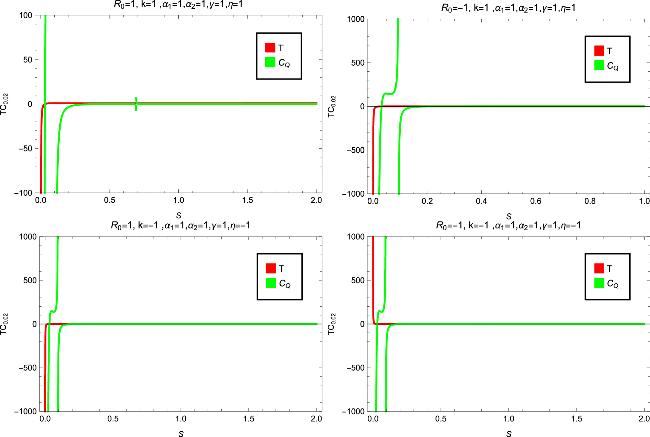
Figure 1. The temperature T and heat capacity CQ versus entropy S for fixed parameters, Q = 0.02, ${f}_{{R}_{0}}=0.1$, α1 = α2 = $\gamma$ = 1 and η = ±1. |
Moreover, we apply geometrothermodynamics to study the phase transition of (A)dS black holes in F(R) gravity. By defining one thermodynamic variable as the thermodynamic potential and taking additional thermodynamic quantities into consideration as extended parameters, the geometrothermodynamics method creates a thermodynamical metric or thermodynamic phase space. The system's phase-transition points can be found by computing this thermodynamical metric's Ricci scalar and locating its divergence point (S). For this objective, different thermodynamic metrics have been designed to construct a geometric phase space based on thermodynamic quantities. A number of metrics, such as the well-known Weinhold [25], Ruppeiner [26, 27] and Quevedo metrics, have been developed to assess the geometrothermodynamics of black holes [28]. As previously noted, concerns have been raised regarding their exact use in assessing different kinds of black holes. In recent research, a new metric known as the HPEM metric was proposed to overcome these difficulties [29]. In this part, we investigate the geometrothermodynamics technique, as specified by the HPEM metric for the phase transition of topological phantom (A)dS black holes in the non-extended phase space. The HPEM metric is defined as [29]2.27 ), $M=\frac{\partial M}{\partial S}=0$ for bound and ${M}_{SS}=\frac{{\partial }^{2}M}{\partial {S}^{2}}=0$ for phase-transition points. If we look at equation (2.31 ), we can see that the roots and divergence points of the heat capacity equal the divergences of the HPEM's Ricci scalar. Basically, the numerator and denominator of the heat capacity are included in the denominator of the Ricci scalar in the HPEM metric (see equation (2.25 )). The roots and critical points of phase transitions in the heat capacity essentially correspond with the divergence points of the Ricci scalar in the HPEM metric. As a result, all relevant physical limitations and phase-transition critical points are contained in the divergences of the Ricci scalar in the HPEM metric. This confirms the HPEM measure as a useful tool to investigate the bound and phase-transition properties of these kinds of black holes.
$\begin{eqnarray}{\rm{d}}{s}^{2}=\frac{S{M}_{S}}{{M}_{QQ}^{3}}\left(-{M}_{SS}{\rm{d}}{S}^{2}+{M}_{QQ}{\rm{d}}{Q}^{2}\right),\end{eqnarray}$
where ${M}_{S}=\frac{\partial M}{\partial S}$, ${M}_{SS}=\frac{{\partial }^{2}M}{\partial {S}^{2}}$ and ${M}_{QQ}=\frac{{\partial }^{2}M}{\partial {Q}^{2}}$. We consider the denominator of the Ricci scalar of the HPEM to look for divergence points of this scalar quantity. Specifically, we are interested in knowing the nature of the denominator since it plays a critical role in defining how the HPEM's Ricci scalar behaves [29]. The denominator of the HPEM's Ricci scalar is as follows $\begin{eqnarray}denom(R)=2{S}^{3}{M}_{S}^{3}{M}_{SS}^{2}.\end{eqnarray}$
Thus, to conduct a proper evaluation of changes that occur in the phase transitions in the field of geometrothermodynamics, it is necessary that the thermodynamic Ricci scalar shows divergence at certain points, as previously shown. These points of divergence are denoted by equation (Moreover, Figure 2 presents the variation of temperature (T), heat capacity (CQ), and Ricci curvature (R) with entropy (S) for fixed parameters fR0 = 0.1, α1 = 1, α2 = 1,$\gamma$ = 1, and Q = 0.02, using different scales of η and R0. The two upper panels correspond to charged (A)dS black holes in F(R)gravity for k = +1 and k = 1, while the two lower panelsillustrate the phantom (A)dS black holes for the samecurvature values. The hatched regions in the figurerepresent the physically meaningful and locally stableconfigurations of these black holes.
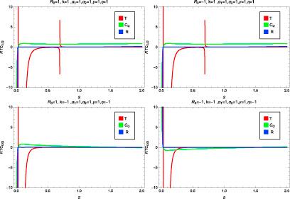
Figure 2. The temperature T, heat capacity CQ and Ricci curvature R versus entropy S for fixed values of the parameter ${f}_{{R}_{0}}$ = 0.1, α1 = 1, α2 = 1, $\gamma$ = 1 and Q = 0.02 with different scales η and R0. |
3. Thermal quantities
In this section, we focus on detailing various thermodynamic properties of topological phantom (A)dS black holes within the framework of F(R) gravity. The Gibbs potential has the capability to predict the global stability of a thermodynamic system in the grand-canonical ensemble, and any value of G that is negative means that the system is globally stable. On the other hand, in the canonical ensemble, the global stability is confirmed using the Helmholtz free energy, which is also required to be negative. Consequently, the goal of the discussion is to analyze the global stability of (A)dS black holes in F(R) gravity using both the Gibbs potential and Helmholtz free energy. The Gibbs potential is defined by the following equation
$\begin{eqnarray}G=M(S,Q)-TS-\eta UQ.\end{eqnarray}$
By inserting the values of corresponding quantities, we can find the Gibbs potential as $\begin{eqnarray}\begin{array}{l}G=-16{\pi }^{2}{\alpha }_{1}^{2}{\alpha }_{2}\eta {Q}^{2}({f}_{{R}_{0}}+1)(-{\alpha }_{1}({f}_{{R}_{0}}+1)+\,{({f}_{{R}_{0}}+1)}^{2}({\alpha }_{1}^{2}+2{\alpha }_{2}{\alpha }_{1}(\gamma S+1)\\ +\,{\alpha }_{2}^{2}{(\gamma S-1)}^{2}){)}^{\frac{1}{2}}+{\alpha }_{2}({f}_{{R}_{0}}+1)(\gamma S-1))+\,\frac{2}{3{\alpha }_{2}{({f}_{{R}_{0}}+1)}^{2}}(-{\alpha }_{1}({f}_{{R}_{0}}+1)\\ +\,\sqrt{{({f}_{{R}_{0}}+1)}^{2}({\alpha }_{1}^{2}+2{\alpha }_{2}{\alpha }_{1}(\gamma S+1)+{\alpha }_{2}^{2}{(\gamma S-1)}^{2})}+\,{\alpha }_{2}({f}_{{R}_{0}}+1)(\gamma S-1){)}^{2}\\ \times \,(6{\alpha }_{1}{\alpha }_{2}k{({f}_{{R}_{0}}+1)}^{2}+{R}_{0}(\sqrt{{({f}_{{R}_{0}}+1)}^{2}({\alpha }_{1}^{2}+2{\alpha }_{2}{\alpha }_{1}(\gamma S+1)+{\alpha }_{2}^{2}{(\gamma S-1)}^{2})}\\ -\,({f}_{{R}_{0}}+1)({\alpha }_{1}+{\alpha }_{2}(1-\gamma S))))-\,(\gamma S({\alpha }_{1}({f}_{{R}_{0}}+1)+{({f}_{{R}_{0}}+1)}^{2}({\alpha }_{1}^{2}+2{\alpha }_{2}{\alpha }_{1}\\ \times \,(\gamma S+1)+{\alpha }_{2}^{2}{(\gamma S-1)}^{2}){)}^{\frac{1}{2}}+{\alpha }_{2}({f}_{{R}_{0}}+1)(\gamma S-1))(-({\alpha }_{1}{\alpha }_{2}({f}_{{R}_{0}}+1)\\ \times \,({\alpha }_{1}({f}_{{R}_{0}}+1)(k+8{\pi }^{2}{\alpha }_{2}\eta {Q}^{2})-\,k{({f}_{{R}_{0}}+1)}^{2}({\alpha }_{1}^{2}+2{\alpha }_{2}{\alpha }_{1}(\gamma S+1)+{\alpha }_{2}^{2}\\ \times \,{(\gamma S-1)}^{2}){)}^{\frac{1}{2}}-{\alpha }_{2}k({f}_{{R}_{0}}+1)(\gamma S-1))))+\,{R}_{0}({\alpha }_{1}^{2}({f}_{{R}_{0}}+1)+{\alpha }_{1}(2{\alpha }_{2}\\ \times \,({f}_{{R}_{0}}+1)-\,\sqrt{{({f}_{{R}_{0}}+1)}^{2}({\alpha }_{1}^{2}+2{\alpha }_{2}{\alpha }_{1}(\gamma S+1)+{\alpha }_{2}^{2}{(\gamma S-1)}^{2})})+{\alpha }_{2}\\ \times \,(\gamma S-1)\,(\sqrt{{({f}_{{R}_{0}}+1)}^{2}({\alpha }_{1}^{2}+2{\alpha }_{2}{\alpha }_{1}(\gamma S+1)+{\alpha }_{2}^{2}{(\gamma S-1)}^{2})}+{\alpha }_{2}\\ \times \,({f}_{{R}_{0}}+1)(\gamma S-1))))({({f}_{{R}_{0}}+1)}^{2}({\alpha }_{1}^{2}+\,2{\alpha }_{2}{\alpha }_{1}(\gamma S+1)+{\alpha }_{2}^{2}{(\gamma S-1)}^{2}){)}^{-1}{)}^{\frac{1}{2}}\\ \times \,(2\sqrt{2}{\alpha }_{1}^{3}{\alpha }_{2}^{2}{({f}_{{R}_{0}}+1)}^{3}\left(\frac{1}{{\alpha }_{1}{\alpha }_{2}{({f}_{{R}_{0}}+1)}^{2}}\right.-\,{\alpha }_{1}({f}_{{R}_{0}}+1)+{({f}_{{R}_{0}}+1)}^{2}({\alpha }_{1}^{2}\\ {\left.+\,2{\alpha }_{2}{\alpha }_{1}(\gamma S+1)+{\alpha }_{2}^{2}{(\gamma S-1)}^{2})\right)}^{\frac{1}{2}}+\,{\alpha }_{2}({f}_{{R}_{0}}+1)(\gamma S-1){)}^{\frac{-3}{2}})).\end{array}\end{eqnarray}$
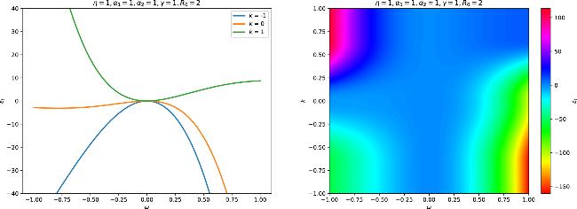
In figure 3, we have depicted the Gibbs free energy G plotted against entropy S with fixed parameters α1 = 1, α2, $\gamma$ = 1, Q = 0.02 and ${f}_{{R}_{0}}=0.1$. The graph's behavior aids in assessing local stability. To examine global stability, it is crucial to consider G being less than zero. Our analysis involves the plotting of four graphs, revealing certain outcomes. For η = 1 and R0 = 2, when considering the charged(A)dS black hole with k = 0, k = 1 and k = -1, the graph shows a downward trajectory for k = -1 and an upward trajectory for k = 0, k = 1, followed by a descent. Therefore, with the specified parameters, the charged (A)dS black hole seems stable for k = -1 and transiently stable for k = 1 and k = 0. For η = 1 and R0 = -2, when considering the charged (A)dS black hole with k = 0, k = 1 and k = -1, the charged (A)dS black hole seems stable for k = 1 and k = 0, and transiently stable for k = - 1. For η = - 1 and R0 = 2, the graph illustrates the behavior of the phantom (A)dS black hole in F(R) gravity with large entropy, by considering three cases k = 0, k = 1 and k = -1. Therefore, based on the graph and specified parameters, the phantom (A)dS black hole appears to be globally stable for k = 1, while it is globally unstable for k = -1 and k = 0. For η = -1 and R0 = -2, the graph illustrates the behavior of the phantom (A)dS black hole in F(R) gravity with large entropy, by considering three cases k = 0, k = 1 and k = - 1. Therefore, based on the graph and specified parameters, the phantom (A)dS black hole appears to be globally stable for k = 0 while it is globally unstable for k = -1 and k = 1. In figures 1-3, the parameters Q = 0.02, ${f}_{{R}_{0}}=0.1$ and α1 = α2 = $\gamma$ = 1, where Q = 0.02 ensures subextremal black holes (charge-to-mass ratio Q/M « 1), avoiding extremal limits. Here, ${f}_{{R}_{0}}=0.1$ reflects perturbative F(R) corrections (|f(R)| « R), consistent with solar system tests [9], and α1 = α2 = $\gamma$ = 1 simplifies the generalized entropy to a symmetric form, enabling direct comparison with Tsallis (α2 = 0) and Barrow (α1 = 0) entropies.
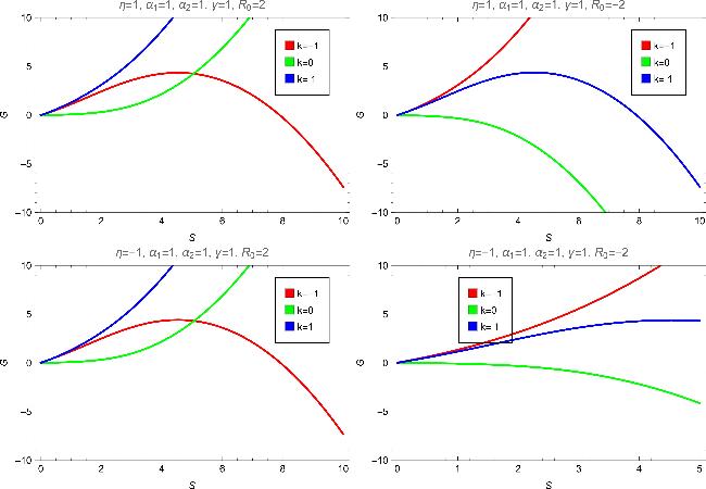
Figure 3. The Gibbs free energy G plotted versus entropy S with fixed parameters. |
Moreover, the Helmholtz free energy is defined as 2.23 ) and (2.24 ), we can get the Helmholtz free energy as
$\begin{eqnarray}{{\rm{F}}}_{{\rm{H}}{\rm{F}}{\rm{E}}}(T,Q)=M(S,Q)-TS.\end{eqnarray}$
Using equations ( $\begin{eqnarray}\begin{array}{l}F(T,Q)=16{\alpha }_{1}^{2}{\alpha }_{2}\eta {\pi }^{2}{Q}^{2}({f}_{{R}_{0}}+1)(-{\alpha }_{1}({f}_{{R}_{0}}+1)+{({f}_{{R}_{0}}+1)}^{2}({\alpha }_{1}^{2}+2{\alpha }_{2}{\alpha }_{1}(\gamma S+1)\\ \,+\,{\alpha }_{2}^{2}{(\gamma S-1)}^{2}){)}^{\frac{1}{2}}+{\alpha }_{2}({f}_{{R}_{0}}+1)(\gamma S-1))+\frac{1}{3{\alpha }_{2}{({f}_{{R}_{0}}+1)}^{2}}\\ \,\times \,(-{\alpha }_{1}({f}_{{R}_{0}}+1)+\sqrt{{({f}_{{R}_{0}}+1)}^{2}({\alpha }_{1}^{2}+2{\alpha }_{2}{\alpha }_{1}(\gamma S+1)+{\alpha }_{2}^{2}{(\gamma S-1)}^{2})}\\ \,+\,{\alpha }_{2}({f}_{{R}_{0}}+1){(\gamma S-1)}^{2}(6{\alpha }_{1}{\alpha }_{2}k{({f}_{{R}_{0}}+1)}^{2}+{R}_{0}(-(({f}_{R}+1)({\alpha }_{1}+{\alpha }_{2}\\ \,\times \,(1-\gamma S)))+\sqrt{{({f}_{{R}_{0}}+1)}^{2}({\alpha }_{1}^{2}+2{\alpha }_{2}{\alpha }_{1}(\gamma S+1)+{\alpha }_{2}^{2}{(\gamma S-1)}^{2})}))\\ \,-\,(S\gamma {\alpha }_{1}({f}_{{R}_{0}}+1)+\sqrt{{({f}_{{R}_{0}}+1)}^{2}({\alpha }_{1}^{2}+2{\alpha }_{2}{\alpha }_{1}(\gamma S+1)+{\alpha }_{2}^{2}{(\gamma S-1)}^{2})}\\ \,+\,{\alpha }_{2}({f}_{{R}_{0}}+1)(\gamma S-1)(-({\alpha }_{1}{\alpha }_{2}({f}_{{R}_{0}}+1)({\alpha }_{1}({f}_{{R}_{0}}+1)(k+8{\alpha }_{2}\eta {\pi }^{2}{Q}^{2})-k\\ \,\times \,\sqrt{{({f}_{{R}_{0}}+1)}^{2}({\alpha }_{1}^{2}+2{\alpha }_{2}{\alpha }_{1}(\gamma S+1)+{\alpha }_{2}^{2}{(\gamma S-1)}^{2})}-{\alpha }_{2}k({f}_{{R}_{0}}+1)\\ \,\times \,(\gamma S-1)))+{R}_{0}({\alpha }_{1}^{2}({f}_{{R}_{0}}+1)+{\alpha }_{1}(2{\alpha }_{2}({f}_{{R}_{0}}+1)-{({f}_{{R}_{0}}+1)}^{2}({\alpha }_{1}^{2}\\ \,+\,2{\alpha }_{2}{\alpha }_{1}(\gamma S+1)+{\alpha }_{2}^{2}{(\gamma S-1)}^{2}){)}^{\frac{1}{2}})\\ \,+\,{\alpha }_{2}(\gamma S-1)\,(\sqrt{{({f}_{{R}_{0}}+1)}^{2}({\alpha }_{1}^{2}+2{\alpha }_{2}{\alpha }_{1}(\gamma S+1)+{\alpha }_{2}^{2}{(\gamma S-1)}^{2})}\\ \,+\,{\alpha }_{2}({f}_{{R}_{0}}+1)(\gamma S-1))))({({f}_{{R}_{0}}+1)}^{2}({\alpha }_{1}^{2}+2{\alpha }_{2}{\alpha }_{1}(\gamma S+1)+{\alpha }_{2}^{2}\\ \,\times \,{(\gamma S-1)}^{2})){)}^{\frac{-1}{2}}(2\sqrt{2}{\alpha }_{1}^{3}{\alpha }_{2}^{2}{({f}_{{R}_{0}}+1)}^{3}\times \left(\frac{1}{{\alpha }_{1}{\alpha }_{2}{({f}_{{R}_{0}}+1)}^{2}}-{\alpha }_{1}({f}_{{R}_{0}}+1)\right.\\ \,+\,\sqrt{{({f}_{{R}_{0}}+1)}^{2}({\alpha }_{1}^{2}+2{\alpha }_{2}{\alpha }_{1}(\gamma S+1)+{\alpha }_{2}^{2}{(\gamma S-1)}^{2})}+{\alpha }_{2}({f}_{{R}_{0}}+1)\\ \,{\left.\times \,(\gamma S-1)\right)}^{\frac{-3}{2}}).\end{array}\end{eqnarray}$
In figure 4, the Helmholtz free energy F is graphed against entropy S with fixed parameters while keeping α1 = 1, α2 = 1, $\gamma$ = 1, Q = 0.02 and ${f}_{{R}_{0}}=0.1$ constant. This graph provides insights into local stability. For a comprehensive assessment of global stability, it is essential to consider situations where the Helmholtz free energy F is less than zero. To investigate the global stability of the (A)dS black hole in F(R) gravity, we present four graphs. Our analysis yields noteworthy findings: specifically, when considering η = 1 and R0 = 2 and examining the charged (A)dS black hole scenarios with k = 0,k = -1 and k = 1. This descending trajectory suggests a downward trend in the Helmholtz free energy concerning entropy. In terms of global stability, this implies that the system is stable. For η = 1 and R0 = -2, the charged (A)dS black hole with k = -1 exhibits global stability while, for k = 1 and k = 0, there may be concerns about global instability. For η = -1 and R0 = 2, the phantom (A)dS black hole with k = 1 and k = 0 appears to be globally stable, while there may be concerns about global instability for k = -1. For η = -1 and R0 = -2, the phantom (A)dS black hole with small entropy appears to exhibit transient instability for k = 1, stabilization for k = -1 and instability for k = 0. The interpretation of stability involves considering the trends in Helmholtz free energy with respect to entropy and assessing whether the system tends towards higher or lower energy states.
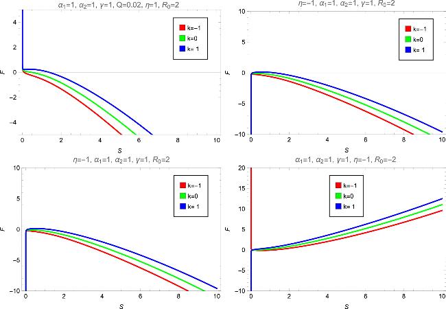
Figure 4. The Helmholtz free energy F plotted versus entropy S with some fixed parameters. |
To gain a more comprehensive understanding of global stability, we have generated graphs depicting the Gibbs free energy G and Helmholtz free energy F in relation to entropy S, employing various parameter values. Throughout this analysis, we maintained fixed values for specific parameters, namely, Q = 0.02 and${f}_{{R}_{0}}=0.1$, as illustrated in figure 5. Upon comparing these perspectives, distinctive behavior in the global stability of black holes within the context of F(R) gravity becomes apparent. In a general context, when examining charged (A)dS black holes with topological constants η = 1 and R0 = 2, the Gibbs free energy tends to exhibit stability where k = -1, while it shows instability for k = 0 and k = 1. On the other hand, the Helmholtz free energy graph indicates stability for k = 0, k = 1 and k = -1. Employing the Gibbs potential, an examination of charged dS black holes with a topological constant η = 1 and a fixed value of R0 = -2, α1 = α2 = $\gamma$ = 1 reveals that the black hole is stable when k takes values of 0 and 1, while it becomes unstable for k = - 1. In contrast, the Helmholtz free energy graph illustrates instability for k = 0, k = -1 and k = 1.
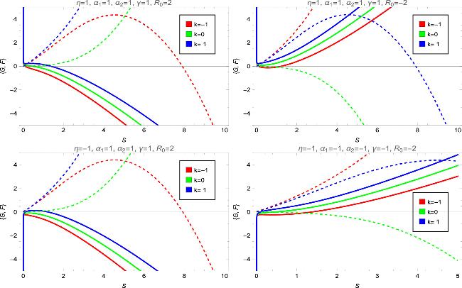
Figure 5. The Gibbs potential G and Helmholtz free energy F plotted versus entropy S with fixed parameters α1 = 1, α2 = 1, $\gamma$ = 1, ${f}_{{R}_{0}}$ = 0.1 and Q = 0.02. Top panel: for η = 1 and R0 = 2, R0 = -2 for different values of k. Bottom panel: for η = -1 and R0 = 2, R0 = -2 for different values of k. |
When comparing both black holes, it is evident that the stability characteristics differ based on the topological constant. For the charged (A)dS black holes, stability is observed for k = -1 while, for charged (A)dS black holes, stability is found for k = 0 and k = 1. The contrasting behavior in stability highlights the sensitivity of the black hole system to changes in the topological constant. When comparing this with the previous scenarios, it is notable that the stability behavior varies depending on the specific combination of parameters. Unlike the charged (A)dS and dS black holes, the phantom (A)dS black hole shows stability for k = -1 but also demonstrates stability for the other values of k = 0 and k = ±1, according to the Helmholtz free energy graph. These distinctions underscore the nuanced and parameter-dependent nature of black hole stability in the context of different topological constants. When comparing this with the previous scenarios, it is notable that the phantom dS black hole exhibits stability only for k = 0 in contrast to the phantom (A)dS black hole, which showed stability for k = -1. Moreover, the Helmholtz free energy graph highlights overall instability for all values of k, emphasizing the nuanced nature of stability patterns that are dependent on the specific parameters of the black hole.
The compressibility factor Z quantifies how real gases differ from the ideal gas behavior. It is calculated using the formula 2.14 ) and (3.7 ), the equation of state P(T, V) can be obtained as
$\begin{eqnarray}Z=\frac{PV}{T}.\end{eqnarray}$
For this calculation, pressure P is defined as $\begin{eqnarray}P=-\frac{{\rm{\Lambda }}}{8\pi }=\frac{{R}_{0}}{32\pi },\end{eqnarray}$
and volume V is given by $\begin{eqnarray}V=\frac{4}{3}\pi {r}_{+}^{3},\end{eqnarray}$
with r denoting the system's radius. Now, using equations ( $\begin{eqnarray}P(T,V)=\frac{0.0003758\left(2145.0294T{V}^{2}({f}_{{R}_{0}}+1)-275{V}^{5/3}k+714.2948V\eta {q}^{2}\right)}{{V}^{7/3}}.\end{eqnarray}$
To find the critical points, we use the conditions [4, 30-32]
$\begin{eqnarray}{P}_{c}=\frac{2.5\times 1{0}^{-8}\left(\frac{8.12\times 1{0}^{6}{\eta }^{3}({f}_{R0}+1){q}^{6}\left(\frac{3.8\times 1{0}^{21}\eta {q}^{2}}{{\left(\frac{{\eta }^{3}{q}^{6}}{{k}^{3}}\right)}^{7/6}}-\frac{1.16\times 1{0}^{22}k}{{\left(\frac{{\eta }^{3}{q}^{6}}{{k}^{3}}\right)}^{5/6}}\right)}{{k}^{3}\left(-\frac{1.79\times 1{0}^{23}{f}_{R0}}{{\left(\frac{{\eta }^{3}{q}^{6}}{{k}^{3}}\right)}^{2/3}}-\frac{1.79\times 1{0}^{23}}{{\left(\frac{{\eta }^{3}{q}^{6}}{{k}^{3}}\right)}^{2/3}}\right)}-263677k{\left(\frac{{\eta }^{3}{q}^{6}}{{k}^{3}}\right)}^{5/6}+43946.2\eta {q}^{2}\sqrt{\frac{{\eta }^{3}{q}^{6}}{{k}^{3}}}\right)}{{\left(\frac{{\eta }^{3}{q}^{6}}{{k}^{3}}\right)}^{7/6}},\end{eqnarray}$
$\begin{eqnarray}{T}_{c}=\frac{\frac{3.9\times 1{0}^{21}\eta {q}^{2}}{{\left(\frac{{\eta }^{3}{q}^{6}}{{k}^{3}}\right)}^{7/6}}-\frac{1.16172\times 1{0}^{22}k}{{\left(\frac{{\eta }^{3}{q}^{6}}{{k}^{3}}\right)}^{5/6}}}{-\frac{1.79\times 1{0}^{23}{f}_{R0}}{{\left(\frac{{\eta }^{3}{q}^{6}}{{k}^{3}}\right)}^{2/3}}-\frac{1.79\times 1{0}^{23}}{{\left(\frac{{\eta }^{3}{q}^{6}}{{k}^{3}}\right)}^{2/3}}},\end{eqnarray}$
$\begin{eqnarray}{V}_{c}=61.5\sqrt{\frac{{\eta }^{3}{q}^{6}}{{k}^{3}}}.\end{eqnarray}$
In figures 4-6, the topological constant, k = 0, ±1, represents flat (k = 0), spherical (k = 1) and hyperbolic (k = -1) horizons, which are standard in cosmological black hole studies [33]. When R0 = ±2, this models AdS (R0 = -2) and dS (R0 = +2) curvature scales, aligned with holographic duality [34] and dark energy scenarios [35].When η = ±1, this distinguishes phantom (η = -1) and Maxwell (η = +1) fields, probing negative or positive energy densities.
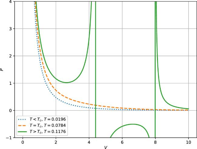
Figure 6. Isotherms on the P-V diagram illustrating phase behavior at T = 0.0531, T = 0.1061 and T = 0.1592. |
Using equation (3.8 ) in equation (3.5 ), we can get the resulting expression for Z
$\begin{eqnarray}Z=\frac{0.0003758\left(2145.0294T{V}^{2}({f}_{{R}_{0}}+1)-275{V}^{5/3}k+714.2948V\eta {q}^{2}\right)}{{V}^{4/3}T}.\end{eqnarray}$
Figure 7 represents the variation of the compressibility factor Z with respect to pressure for different temperatures in an (A)dS black hole. The nature of the relationship between Z and pressure is further described by the plot that shows that while the pressure is low, Z increases. This pattern shows differences compared with the conventional compressibility factor for an (A)dS black hole system and an ideal gas in which Z = 1. Further, the compressibility factor at the critical point for our system is higher: in fact, above three times a van der Waals fluid at Zc = 0.375 [36].
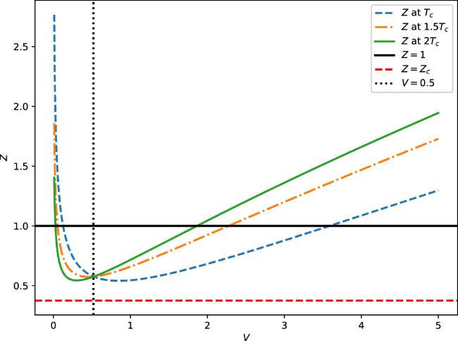
Figure 7. The compressibility factor Z plotted versus volume V for different temperatures. |
The isothermic compressibility (κT) provides the study of phase transitions as it reveals the kind of response the thermodynamic system exhibits at a fixed temperature with respect to pressure. The isothermal compressibility is defined as 3.13 ), (3.8 ) and (2.14 ), we obtain
$\begin{eqnarray}{\kappa }_{T}=-\frac{1}{V}{\left(\frac{{\rm{d}}V}{{\rm{d}}P}\right)}_{T},\end{eqnarray}$
where V is the volume, P is the pressure and T is the temperature. After substituting the relations from equations ( $\begin{eqnarray}\begin{array}{l}{\kappa }_{T}=\frac{128\cdot {2}^{1/3}{\pi }^{11/3}{({r}_{+}^{3})}^{11/3}}{27\cdot {3}^{2/3}\left(0.01{({r}_{+}^{3})}^{7/3}(714.3\eta {q}^{2}-\frac{2750}{3}{2}^{1/3}k{\left(\frac{\pi }{3}\right)}^{2/3}{({r}_{+}^{3})}^{2/3}+17970.2(1+{f}_{{R}_{0}}){r}_{+}^{3}(-\frac{\eta {q}^{2}}{4(1+{f}_{{R}_{0}})\pi {r}_{+}^{3}}+\frac{k}{4\pi {r}_{+}}\right.}\\ \times \,\frac{1}{+\frac{{R}_{0}{r}_{+}}{16\pi }))-0.006{({r}_{+}^{3})}^{4/3}\left(2992.03\eta {q}^{2}{r}_{+}^{3}-\frac{2200\cdot {2}^{1/3}k{\pi }^{5/3}{({r}_{+}^{3})}^{5/3}}{3\cdot {3}^{2/3}}+37636.6(1+{f}_{{R}_{0}}){r}_{+}^{6}\left(-\frac{\eta {q}^{2}}{4(1+{f}_{{R}_{0}})\pi {r}_{+}^{3}}\right.\right.}\\ \times \,\frac{1}{+\left.\left.\left.\frac{k}{4\pi {r}_{+}}+\frac{{R}_{0}{r}_{+}}{16\pi }\right)\right)\right)}.\end{array}\end{eqnarray}$
In figure 8, it is clear that black holes with positive isothermal compressibility, whether they are big or small, are thermodynamically stable. On the other hand, mid-sized black holes find themselves in the region of instability, characterized by negative values of κT. Since an (A)dS phantom black hole radiates energy, quantum fluctuations lead to the creation of particles and antiparticles beyond the event horizon rh. In fact, through the quantum tunneling phenomenon, particles with positive energy may escape from the innermost regions of the black hole's vicinity, giving rise to Hawking radiation and the associated evaporation process. The rate at which the black hole evaporates depends on its energy emission rate, which can be observed by an observer located far from the black hole. For such an observer, the black hole's shadow corresponds to a high-energy absorption cross-section, which characterizes how the black hole interacts with incoming radiation. The limiting value of the absorption cross-section is approximately
$\begin{eqnarray}{\sigma }_{\,\rm{lim}\,}\approx \pi {r}_{+}^{2}.\end{eqnarray}$
Therefore, the energy emission rate of the black hole is given by $\begin{eqnarray}\frac{{{\rm{d}}}^{2}\epsilon }{{\rm{d}}\omega {\rm{d}}t}=\frac{2{\pi }^{2}{\sigma }_{\,\rm{lim}\,}}{{{\rm{e}}}^{\omega /T}-1}{\omega }^{3},\end{eqnarray}$
where T represents the modified temperature. The emission rate as a function of the event horizon rh and the parameters of the black hole equation of state for the (A)dS phantom black hole. To account for the full thermodynamic properties of the (A)dS phantom black hole, we incorporate the four-parameter entropy, which encodes the entropy of the black hole as a function of its mass, charge, pressure and volume. The final expression for the energy emission rate can then be derived as a function of both the event horizon radius rh and the four-parameter entropy, incorporating the underlying microstate configuration of the black hole.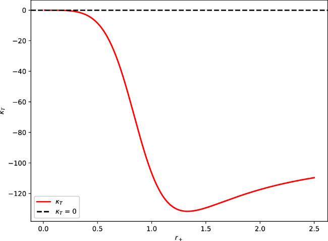
Figure 8. The κT as a function of the radius r+, calculated using the constants η = 1.0, k = 1.0, R0 = 2.0, q = 0.5 and ${f}_{{R}_{0}}=0.1$. The dashed line indicates where κT = 0, serving as a critical point. |
The behavior of the energy emission rate as a function of ω is presented in figure 9 for different values of k. We see a noticeable peak in the energy emission rate for the (A)dS black hole. This peak is noticeably reduced when the generalized four-parameter entropy function is incorporated, suggesting that the emission rate is dampened under nonextensive statistics. This first implies that black hole evaporation takes place more slowly. Moreover, for large ω the effect estimated from k statistics is not resolved as distinct from that predicted by the Boltzmann-Gibbs formula. In figures 7-9, the non-commutative parameter θ = 0.1, in particular, reflects intermediate space-time fuzziness, avoiding singularities while preserving semiclassical behavior [36]. When β = 1, this balances Generalized Uncertainty Principle (GUP) corrections to entropy, consistent with quantum gravity bounds (β0 ~ 1) [37].
Figure 9. The energy emission rate as a function of ω for different settings of free parameters and k is shown. |
3.1. Qualitative and quantitative comparison
For a Schwarzschild black hole (Q = 0, k = 1, R0 = 0):
1. Heat Capacity:
a. Bekenstein-Hawking: CQ = - 8πM2, universally negative (thermodynamically unstable).
b. Generalized Entropy: CQ diverges (figure 1), signaling phase transition to stable configurations (CQ > 0) for S.
2. Energy Emission Rate:
a. Bekenstein-Hawking: standard Hawking decay $\frac{{\rm{d}}M}{{\rm{d}}t}\propto -{M}^{-2}$, leading to total evaporation.
b. Generalized Entropy: suppressed emission (figure 9) with $\frac{{\rm{d}}M}{{\rm{d}}t}\to 0$ as M → Mmin ≈ 0.5Minitial, predicting stable remnants.
3. Phase Transitions:
a. Bekenstein-Hawking: no phase transitions (monotonic CQ).
b. Generalized Entropy: second-order transition.
4. Concluding remarks
In the present work, we have investigated the topological phantom (A)dS black holes via various thermodynamic quantities as well as geometries in the presence of recently proposed generalized entropy for a specific and useful choice of constant parameters. In this way, we have displayed the temperature and specific heat in figure 1, which depict the transition of black holes from locally unstable to locally stable regions by crossing the phase-transition border. In figure 2, we have checked the behavior of particles near the horizon through thermodynamic geometry (HPEM), in which black hole solutions exhibit attractive/repulsive behavior, depending upon the choices of constant parameters. For global stability, the Gibbs free energy exhibits stable behavior for all black hole solutions (k = 0, 1, -1); however, the black hole solution corresponding to k = -1 depicts unstable behavior for a large horizon radius (figure 3). On the other hand, Helmholtz free energy also provides the stable behavior of black hole solutions in most cases of constant parameters (figure 4). In figure 5, these findings highlight the intricate dependence of black hole stability on both topological and parametric factors. In figure 6, it has been observed that with the P-V isotherms of (A)dS black holes at T > Tc, T = Tc and T < Tc, (A)dS black holes exhibit rich thermodynamic phases. In figure 7, one can see that at low pressures, the compressibility factor Z grows beyond the ideal gas value, revealing distinctive deviations in the (A)dS black hole system. Figure 8 confirms the thermodynamic stability of positive isothermal compressibility black holes in agreement with the above existent literature and shows the instability of mid-sized black holes. Furthermore, figure 9 exhibits that generalized four-parameter entropy function results significantly impact on the energy emission rate of (A)dS black holes, which implies a slower evaporation process. The black hole behavior is shown in these findings to be influenced by the statistical frameworks. The physical realism and theoretical consistency of parameters are chosen. Real-world black holes are characterized by small charge values (Q « M), ensuring minimum charge due to the same factors as black hole charge neutralization, namely, rapid neutralization. This takes our F(R)-gravity parameter to ${f}_{{R}_{0}}=0.1$, which is small enough to leave spacetime curvature undisturbed. The model is simplified by the generalized entropy parameters α1 = α2 = $\gamma$ = 1, and allows comparison to classical entropy forms, with β = 1 regulating quantum-classical exchange. In this regime, anti de Sitter (linked to holography) and de Sitter (dark energy) both cover the curvature R0 = ±2 regime, making the cosmological relevance broad.
Within the generalized entropy framework, pathologies of Bekenstein-Hawking thermodynamics are resolved and phase transitions are introduced. It illustrates its usefulness not only in quantum gravitational modeling and prediction of observable remains, but also in the advancement of classical black hole thermodynamics (detail is mentioned in table 2).
Table 2. Key differences between entropy formulations. |
| Property | Bekenstein-Hawking | Generalized entropy | Advantage of generalized entropy |
|---|---|---|---|
| Heat capacity | CQ < 0 (always unstable) | CQ > 0 for S | Stabilizes large black holes |
| Emission rate | Complete evaporation | Remnant formation (Mmin) | Resolves singularity paradox |
| Phase transitions | None | Second-order at S | Enriches thermodynamic phase structure |