


1. Introduction
The Wiedemann-Franz (WF) law has long been a cornerstone of understanding the interaction between electrical and thermal conductivity in metals and was introduced by Jonson [1]. Tang et al developed a hydrodynamic transport model for silicon devices, incorporating the WF law to explore charge carrier behavior and transport properties in silicon [2]. Chien investigated magnetic and giant magnetic transport phenomena in granular solids, highlighting the WF law's significance in magnetic materials [3]. In 1996, both thermal conductance and thermopower have been analyzed for a pure 1D gas and for systems with impurities [4]. Henny et al reported the suppression of breakdown noise in diffuse nanowires using a heating model based on the WF law [5]. Proust et al confirmed the WF law's validity in strongly doped copper oxides in the normal state, extending its applicability to unconventional superconductors [6]. Tanatar et al reported a violation of the WF law in heavy fermionic metals at the quantum critical point [7].
Garg et al demonstrated that in weakly disordered Luttinger liquids, the ratio of thermal conductivity $\kappa $ to electrical conductivity $\sigma $ can deviate significantly from the WF law [8]. Kim et al investigated electrical and thermal transport near the heavy-fermion quantum critical point, finding that the WF ratio can exceed the standard value [9]. In 2013, Universal expressions for conductivity ratios that violate the WF law have also been derived [10]. Lee et al reported a significant, order-of-magnitude breakdown of the WF law in metallic vanadium dioxide near its metal-insulator transition [11]. Brown et al studied transport in clean quantum systems, using the Nernst-Einstein relation to convert the diffusion constant into resistivity [12]. Mason observed that the reduction in thermal conductivity of thin films results in a breakdown of the WF law, demonstrating that the law may not hold under certain conditions [13]. Zeng conducted an in-depth study of nonlinear anomalous transport and proposed a fundamental relationship linking nonlinear anomalous electrical and thermoelectric transport coefficients [14]. Wang et al provided evidence for strong WF law violations observed in cuprates at room temperature [15].
Grounded in the work of Henri Poincare, Thom and others [16], the catastrophe theory can explain the phenomenon of gradual quantitative change to sudden qualitative change, which is a highly generalized mathematical theory that summarizes the rules of non-equilibrium phase transition by several catastrophe models.
In this paper, based on the catastrophe theory, starting from the thermodynamic potential of relativistic degenerate electron gas, by using the non-dimensional analysis we want to derive a generalized WF law to satisfy all conditions including the cryogenic and infinite-temperature limits.
2. The structural-stability-based catastrophe models
For the nonlinear differential equation $\dot{x}=f\left(x,\mu \right)\,$ with the fixed point ${x}_{f}$, we suppose that it is structurally stable at the fixed point. Assuming the existence of perturbations causing $f\left(x,\mu \right)\to f\left(x,\mu \right)+\delta f\left(x,\mu \right)$, the fixed point also generates corresponding perturbations ${x}_{f}\to {x}_{f}+\delta {x}_{f}$ whose movement amplitude is limited by the size of the perturbation $\delta f\left({x}_{f},\mu \right)$, which indicates that $f\left(x,\mu \right)+\delta f\left(x,\mu \right)$ should be structurally stable at ${x}_{f}+\delta {x}_{f}$ for small $\delta {x}_{f}$.
To investigate the stability of the structure of phase trajectory motion, a small amount can be added to the system state equation to perturb the entire vector field. If the perturbed phase diagram of the system is topologically equivalent to the initial phase diagram in the orbital sense, then the original system is structurally stable.
For the gradient system $f\left(x,\mu \right)=-{\rm{\nabla }}V\left(x,\mu \right)$, when the control variable $\mu \in {R}^{k}$ changes, to ensure that the fixed point remains structurally stable for $f\left(x,\mu \right)=0$, Thom defined a set that satisfies
$\begin{eqnarray}\left\{\begin{array}{lll}{\rm{\nabla }}V\left(x,\mu \right) & = & 0\\ {\rm{d}}{\rm{e}}{\rm{t}}\left|\displaystyle \frac{{\partial }^{2}V\left(x,\mu \right)}{\partial {x}_{i}{x}_{j}}\right| & = & 0\end{array},\right.\end{eqnarray}$
which is called the basic mutation K set in the control space. The mutation set K is a set of bifurcation points, which is a k-1 dimensional manifold in the control space, and the mutation set of $V\left(x,\mu \right)$ is structurally stable.Thom analyzed the stability problem of the basic mutation set satisfying condition (8) in the zero-solution neighborhood and proposed a mutation theory based on the potential function $V\left(x,\mu \right)$. According to Thom's classification theorem, as long as the number of control variables $\mu $ that cause mutations does not exceed 4, the various mutation processes in nature can be grasped using seven basic potential function models. The mutation phenomena belonging to the same model have a set of differentially homomorphic mutations.
According to the catastrophe theory, for any phase transition process there exist seven types of elementary catastrophe models with the corresponding different potential functions as shown in table 1.
Table 1. The elementary catastrophe types [17]. |
| The catastrophe types | Corresponding potential functions | No. of variables | No. of parameters |
|---|---|---|---|
| Folding | ${x}^{3}+kx$ | 1 | 1 |
| Cusp | ${x}^{4}+k{x}^{2}+nx$ | 1 | 2 |
| Swallowtail | ${x}^{5}+k{x}^{3}+n{x}^{2}+\omega x$ | 1 | 3 |
| Butterfly | ${x}^{6}+t{x}^{4}+k{x}^{3}+n{x}^{2}+\omega x$ | 1 | 4 |
| Hyperbolic umbilical | ${x}^{3}+{y}^{3}+\omega xy-kx-ny$ | 2 | 3 |
| Oval umbilical | ${x}^{3}-x{y}^{2}+\left({x}^{2}+{y}^{2}\right)-kx+ny$ | 2 | 3 |
| Parabolic umbilical | ${x}^{4}+{x}^{2}y+u{x}^{2}+t{y}^{2}-kx-ny$ | 2 | 4 |
In fact, the stability of these seven mutation models in the zero-solution neighborhood can be extended to the non-zero solution neighborhood of the nonlinear differential equation $\dot{x}=f\left(x,\mu \right)$ based on the principle of linear stability.
In the following, the swallowtail catastrophe model is adopted to obtain a general WF law to overcome the shortcomings of the traditional law.
3. The general Wiedemann-Franz law derived
In electrically conductive solids, the WF law requires thermal conductivity to be proportional to electrical conductivity, i.e.
$\begin{eqnarray}\begin{array}{c}\displaystyle \frac{\rho }{\sigma }=LT=\displaystyle \frac{{\pi }^{2}}{3}{\left(\displaystyle \frac{{k}_{{\rm{B}}}}{e}\right)}^{2}T,\end{array}\end{eqnarray}$
where $\rho $ is the thermal conductivity, $\sigma $ is the electrical conductivity, T is Kelvin temperature, ${k}_{{\rm{B}}}$ the Boltzmann constant, $e$ the electron charge, and it is shown that although the value of $L$ is roughly constant, it is not entirely the same.It is known that the thermodynamic potential of relativistic degenerate electron gas can be expressed as
$\begin{eqnarray}\begin{array}{c}{\rm{\Omega }}=-\displaystyle \frac{V{\left({k}_{{\rm{B}}}T\right)}^{4}}{3{\pi }^{2}{c}^{3}{ \hbar }^{3}}\displaystyle {\int }_{0}^{\infty }\displaystyle \frac{{z}^{3}{\rm{d}}z}{{{\rm{e}}}^{z-\displaystyle \frac{\mu }{{k}_{{\rm{B}}}T}}+1}=-\displaystyle \frac{{k}_{{\rm{w}}}}{c}V{T}^{4},\end{array}\end{eqnarray}$
where ${k}_{{\rm{w}}}=\tfrac{{{k}_{{\rm{B}}}}^{4}}{3{\pi }^{2}{c}^{2}{{ \hbar }}^{3}}{f}_{1}\left(\tfrac{\mu }{{k}_{{\rm{B}}}T}\right)$ describes the electron-electron interaction, which is with the same dimension as that of the Stefan-Boltzmann constant in blackbody radiation, ${k}_{{\rm{B}}}$ the Boltzmann constant, $T$ is Kelvin temperature, $V$ the volume, ${ \hbar }$ the reduced Plank's constant, c the light speed, $\mu $ the chemical potential of electron gas, and ${f}_{1}\left(\tfrac{\mu }{{k}_{{\rm{B}}}T}\right)=\displaystyle {\int }_{0}^{\infty }\tfrac{{z}^{3}{\rm{d}}z}{{{\rm{e}}}^{z-\displaystyle \tfrac{\mu }{{k}_{{\rm{B}}}T}}+1}$ is a dimensionless univariate function.In addition, the electron density in solids is
$\begin{eqnarray}\begin{array}{c}\bar{n}=\displaystyle \frac{N}{V}=\displaystyle \frac{\sqrt{2}{\left({k}_{{\rm{B}}}T\right)}^{3/2}{m}^{3/2}}{{{\rm{\pi }}}^{2}{ \hbar }^{3}}\displaystyle {\int }_{0}^{\infty }\displaystyle \frac{{z}^{1/2}{\rm{d}}z}{{{\rm{e}}}^{z-\displaystyle \frac{\mu }{{k}_{{\rm{B}}}T}}+1}={n}_{{\rm{w}}}{T}^{3/2},\end{array}\end{eqnarray}$
where m is the electron mass, ${n}_{{\rm{w}}}=\displaystyle \frac{\sqrt{2}{{k}_{{\rm{B}}}}^{3/2}{m}^{3/2}}{{\pi }^{2}{{ \hbar }}^{3}}{f}_{2}\left(\displaystyle \frac{\mu }{{k}_{{\rm{B}}}T}\right)$ is an electron density parameter, ${f}_{2}\left(\displaystyle \frac{\mu }{{k}_{{\rm{B}}}T}\right)=\displaystyle {\int }_{0}^{\infty }\displaystyle \frac{{z}^{1/2}{\rm{d}}z}{{{\rm{e}}}^{z-\displaystyle \frac{\mu }{{k}_{{\rm{B}}}T}}+1}$ is also a dimensionless univariate function.When $T\to 0$, the function $\displaystyle \frac{1}{{{\rm{e}}}^{z-\displaystyle \frac{\mu }{{k}_{{\rm{B}}}T}}+1}$ changes to a step function, i.e. it is equal to 1 when $z\lt \displaystyle \frac{\mu }{{k}_{{\rm{B}}}T}$, and it is equal to 0 when $z\gt \displaystyle \frac{\mu }{{k}_{{\rm{B}}}T}$. Thus when $T\to 0$, there is
$\begin{eqnarray}\begin{array}{c}\mathop{\mathrm{lim}}\limits_{T\to 0}{f}_{1}\left(\displaystyle \frac{\mu }{{k}_{{\rm{B}}}T}\right)=\displaystyle {\int }_{0}^{\displaystyle \frac{\mu }{{k}_{{\rm{B}}}T}}{z}^{3}{\rm{d}}z=\displaystyle \frac{1}{4}{\left(\displaystyle \frac{\mu }{{k}_{{\rm{B}}}T}\right)}^{4},\end{array}\end{eqnarray}$
and $\begin{eqnarray}\begin{array}{c}\mathop{\mathrm{lim}}\limits_{T\to 0}{f}_{2}\left(\displaystyle \frac{\mu }{{k}_{{\rm{B}}}T}\right)=\displaystyle {\int }_{0}^{\displaystyle \frac{\mu }{{k}_{{\rm{B}}}T}}{z}^{1/2}{\rm{d}}z=\displaystyle \frac{2}{3}{\left(\displaystyle \frac{\mu }{{k}_{{\rm{B}}}T}\right)}^{3/2},\end{array}\end{eqnarray}$
Thus when $T\to 0$, ${k}_{{\rm{w}}}\propto {T}^{-4}$ and ${n}_{{\rm{w}}}\propto {T}^{-3/2}$.When $\,T\to \infty $, the electron gas will degenerate into an ideal Boltzmann gas, for which the following relation holds: $\mu ={k}_{{\rm{B}}}T\,{\mathrm{ln}}\left[\displaystyle \frac{N}{V}{\left(\displaystyle \frac{2\pi {{ \hbar }}^{2}}{m{k}_{{\rm{B}}}T}\right)}^{3/2}\right]$,Furthermore, by considering ${f}_{1}\left(\displaystyle \frac{\mu }{{k}_{{\rm{B}}}T}\right)$ and ${f}_{2}\left(\displaystyle \frac{\mu }{{k}_{{\rm{B}}}T}\right)$ given in the previous section, it can be concluded that: $\mathop{\mathrm{lim}}\limits_{T\to \infty }{f}_{1}\left(\displaystyle \frac{\mu }{{k}_{{\rm{B}}}T}\right)=\mathop{\mathrm{lim}}\limits_{T\to \infty }{f}_{2}\left(\displaystyle \frac{\mu }{{k}_{{\rm{B}}}T}\right)={\rm{constant}}$. Thus, in the infinite-temperature limit, ${k}_{{\rm{w}}}={\rm{constant}}$ and ${n}_{{\rm{w}}}={\rm{constant}}$.
To derive the WF law, the swallowtail catastrophe model in table 1 is adopted with the temperature $T$ as the variable, since its equilibrium surface is in the form
$\begin{eqnarray}\begin{array}{c}{T}^{4}+k{T}^{2}+nT+\omega =0,\end{array}\end{eqnarray}$
in which the three parameters $\,k$, $n$ and $\omega $ can be expanded, respectively, as $\begin{eqnarray}\begin{array}{c}k\,=A\,{{k}_{{\rm{w}}}}^{{\alpha }_{1}}{{k}_{{\rm{B}}}}^{{\alpha }_{2}}{\sigma }^{{\alpha }_{3}}{\rho }^{{\alpha }_{4}}{e}^{{\alpha }_{5}}{ \hbar }^{{\alpha }_{6}}{\tau }^{{\alpha }_{7}}{{n}_{{\rm{w}}}}^{{\alpha }_{8}}{m}^{{\alpha }_{9}},\end{array}\end{eqnarray}$
$\begin{eqnarray}\begin{array}{c}n\,=B\,{{k}_{{\rm{w}}}}^{{\beta }_{1}}{{k}_{{\rm{B}}}}^{{\beta }_{2}}{\sigma }^{{\beta }_{3}}{\rho }^{{\beta }_{4}}{e}^{{\beta }_{5}}{ \hbar }^{{\beta }_{6}}{\tau }^{{\beta }_{7}}{{n}_{{\rm{w}}}}^{{\beta }_{8}}{m}^{{\beta }_{9}},\end{array}\end{eqnarray}$
$\begin{eqnarray}\begin{array}{c}\omega \,=C\,{{k}_{{\rm{w}}}}^{{\gamma }_{1}}{{k}_{{\rm{B}}}}^{{\gamma }_{2}}{\sigma }^{{\gamma }_{3}}{\rho }^{{\gamma }_{4}}{e}^{{\gamma }_{5}}{ \hbar }^{{\gamma }_{6}}{\tau }^{{\gamma }_{7}}{{n}_{{\rm{w}}}}^{{\gamma }_{8}}{m}^{{\gamma }_{9}},\end{array}\end{eqnarray}$
where $\tau $ is the relaxation time of metals, $A$, $B$ and $C$ are constants to be determined, and all the indices ${\alpha }_{1}$, ${\beta }_{1}$, ${\gamma }_{1}$, … ${\alpha }_{9}$, ${\beta }_{9}$, ${\gamma }_{9}$ are constants to be determined by the non-dimensional analysis below plus the additional temperature-limit conditions. In the temperature limit, according to [15, 18], when $T\to \infty ,$ there is $\rho \propto 1/{T}^{2}$, $\tau \propto 1/T$ and $\sigma \propto 1/T$. On the other hand, when $T\to 0\,{\rm{K}},$ there is $\rho \propto {T}^{3}$, $\tau \propto 1/{T}^{2}$ and $\sigma \propto 1/{T}^{5}$ [19].According to equation (6 ), the dimensions of $k$, $n$, and $\omega $ are $\left[{T}^{2}\right]$, $\left[{T}^{3}\right]$, and $\left[{T}^{4}\right]$, respectively. By introducing the five international standard units, length [m], time [s], mass [kg], temperature [K] and ampere [A], as listed in table 2, there are the following relationships for the indices.
$\begin{eqnarray}\left\{\begin{array}{lll}2{\alpha }_{2}-3{\alpha }_{3}+{\alpha }_{4}+2{\alpha }_{6}-3{\alpha }_{8} & = & 0\\ -3{\alpha }_{1}-2{\alpha }_{2}+3{\alpha }_{3}-3{\alpha }_{4}+{\alpha }_{5}-{\alpha }_{6}+{\alpha }_{7} & = & 0\\ {\alpha }_{1}+{\alpha }_{2}-{\alpha }_{3}+{\alpha }_{4}+{\alpha }_{6}+{\alpha }_{9} & = & 0\\ -4{\alpha }_{1}-{\alpha }_{2}-{\alpha }_{4}-\displaystyle \frac{3{\alpha }_{8}}{2} & = & 2\\ 2{\alpha }_{3}+{\alpha }_{5} & = & 0\end{array},\right.\end{eqnarray}$
$\begin{eqnarray}\begin{array}{c}\left\{\begin{array}{lll}2{\beta }_{2}-3{\beta }_{3}+{\beta }_{4}+2{\beta }_{6}-3{\beta }_{8} & = & 0\\ -3{\beta }_{1}-2{\beta }_{2}+3{\beta }_{3}-3{\beta }_{4}+{\beta }_{5}-{\beta }_{6}+{\beta }_{7} & = & 0\\ {\beta }_{1}+{\beta }_{2}-{\beta }_{3}+{\beta }_{4}+{\beta }_{6}+{\beta }_{9} & = & 0\\ -4{\beta }_{1}-{\beta }_{2}-{\beta }_{4}-\displaystyle \frac{3{\beta }_{8}}{2} & = & 3\\ 2{\beta }_{3}+{\beta }_{5} & = & 0\end{array}\right.,\end{array}\end{eqnarray}$
$\begin{eqnarray}\begin{array}{c}\left\{\begin{array}{lll}2{\gamma }_{2}-3{\gamma }_{3}+{\gamma }_{4}+2{\gamma }_{6}-3{\gamma }_{8} & = & 0\\ -3{\gamma }_{1}-2{\gamma }_{2}+3{\gamma }_{3}-3{\gamma }_{4}+{\gamma }_{5}-{\gamma }_{6}+{\gamma }_{7} & = & 0\\ {\gamma }_{1}+{\gamma }_{2}-{\gamma }_{3}+{\gamma }_{4}+{\gamma }_{6}+{\gamma }_{9} & = & 0\\ -4{\gamma }_{1}-{\gamma }_{2}-{\gamma }_{4}-\displaystyle \frac{3{\gamma }_{8}}{2} & = & 4\\ 2{\gamma }_{3}+{\gamma }_{5} & = & 0\end{array}\right.,\end{array}\end{eqnarray}$
Table 2. The dimensional analysis of all the indices. |
| ${k}_{{\rm{w}}}$ | ${k}_{{\rm{B}}}\,$ | $\sigma $ | ρ | e | ħ | $\tau $ | ${n}_{{\rm{w}}}$ | $m$ | |
|---|---|---|---|---|---|---|---|---|---|
| Length | 0 | 2 | -3 | 1 | 0 | 2 | 0 | -3 | 0 |
| Time | -3 | -2 | 3 | -3 | 1 | -1 | 1 | 0 | 0 |
| Mass | 1 | 1 | -1 | 1 | 0 | 1 | 0 | 0 | 1 |
| Temp | -4 | -1 | 0 | -1 | 0 | 0 | 0 | -3/2 | 0 |
| Ampere | 0 | 0 | 2 | 0 | 1 | 0 | 0 | 0 | 0 |
By solving equation (8 ), we can obtain respectively that
$\begin{eqnarray}\displaystyle \begin{array}{c}k\,=A{{k}_{{\rm{w}}}}^{{\alpha }_{1}}{{k}_{{\rm{B}}}}^{{\alpha }_{2}}{\sigma }^{{\alpha }_{3}}{\rho }^{{\alpha }_{4}}{e}^{-2{\alpha }_{3}}{ \hbar }^{-4{\alpha }_{1}-2{\alpha }_{2}+\displaystyle \frac{3}{2}{\alpha }_{3}-\displaystyle \frac{3}{2}{\alpha }_{4}-2}{\tau }^{-{\alpha }_{1}+\displaystyle \frac{{\alpha }_{3}}{2}+\displaystyle \frac{3}{2}{\alpha }_{4}-2}{{n}_{{\rm{w}}}}^{\displaystyle \frac{-2}{3}\left(4{\alpha }_{1}+{\alpha }_{2}+{\alpha }_{4}+2\right)}{m}^{3{\alpha }_{1}+{\alpha }_{2}-\displaystyle \frac{{\alpha }_{3}}{2}+\displaystyle \frac{{\alpha }_{4}}{2}+2},\end{array}\end{eqnarray}$
$\begin{eqnarray}\displaystyle \begin{array}{c}n=B{{k}_{{\rm{w}}}}^{{\beta }_{1}}{{k}_{{\rm{B}}}}^{{\beta }_{2}}{\sigma }^{{\beta }_{3}}{\rho }^{{\beta }_{4}}{e}^{-2{\beta }_{3}}{ \hbar }^{-4{\beta }_{1}-2{\beta }_{2}+\displaystyle \frac{3}{2}{\beta }_{3}-\displaystyle \frac{3}{2}{\beta }_{4}-3}{\tau }^{-{\beta }_{1}+\displaystyle \frac{{\beta }_{3}}{2}+\displaystyle \frac{3}{2}{\beta }_{4}-3}{{n}_{{\rm{w}}}}^{\displaystyle \frac{-2}{3}\left(4{\beta }_{1}+{\beta }_{2}+{\beta }_{4}+3\right)}{m}^{3{\beta }_{1}+{\beta }_{2}-\displaystyle \frac{{\beta }_{3}}{2}+\displaystyle \frac{{\beta }_{4}}{2}+3,}\end{array}\end{eqnarray}$
$\begin{eqnarray}\displaystyle \begin{array}{c}\omega \,=C{{k}_{{\rm{w}}}}^{{\gamma }_{1}}{{k}_{{\rm{B}}}}^{{\gamma }_{2}}{\sigma }^{{\gamma }_{3}}{\rho }^{{\gamma }_{4}}{e}^{-2{\gamma }_{3}}{ \hbar }^{-4{\gamma }_{1}-2{\gamma }_{2}+\displaystyle \frac{3}{2}{\gamma }_{3}-\displaystyle \frac{3}{2}{\gamma }_{4}-4}{\tau }^{-{\gamma }_{1}+\displaystyle \frac{{\gamma }_{3}}{2}+\displaystyle \frac{3}{2}{\gamma }_{4}-4}{{n}_{{\rm{w}}}}^{\displaystyle \frac{-2}{3}\left(4{\gamma }_{1}+{\gamma }_{2}+{\gamma }_{4}+4\right)}{m}^{3{\gamma }_{1}+{\gamma }_{2}-\displaystyle \frac{{\gamma }_{3}}{2}+\displaystyle \frac{{\gamma }_{4}}{2}+4}.\end{array}\end{eqnarray}$
When $T\to \infty ,$ there are $\rho \propto 1/{T}^{2}$, $\tau \propto 1/T,$ and $\sigma \propto 1/T$ [15, 18]. Thus $\begin{eqnarray}\begin{array}{c}{\sigma }^{{\alpha }_{3}}{\rho }^{{\alpha }_{4}}{\tau }^{-{\alpha }_{1}+\displaystyle \frac{{\alpha }_{3}}{2}+\displaystyle \frac{3}{2}{\alpha }_{4}-2}\propto {T}^{2}\,\to \,{\alpha }_{1}-\displaystyle \frac{3}{2}{\alpha }_{3}-\displaystyle \frac{7}{2}{\alpha }_{4}=0,\end{array}\end{eqnarray}$
$\begin{eqnarray}\begin{array}{c}{\sigma }^{{\beta }_{3}}{\rho }^{{\beta }_{4}}{\tau }^{-{\beta }_{1}+\displaystyle \frac{{\beta }_{3}}{2}+\displaystyle \frac{3}{2}{\beta }_{4}-3}\propto {T}^{3}\,\to {\rm{\ }}{\beta }_{1}-\displaystyle \frac{3}{2}{\beta }_{3}-\displaystyle \frac{7}{2}{\beta }_{4}=0,\end{array}\end{eqnarray}$
$\begin{eqnarray}\begin{array}{c}{\sigma }^{{\gamma }_{3}}{\rho }^{{\gamma }_{4}}{\tau }^{-{\gamma }_{1}+\displaystyle \frac{{\gamma }_{3}}{2}+\displaystyle \frac{3}{2}{\gamma }_{4}-3}\propto {T}^{4}\,\to {\rm{\ }}{\gamma }_{1}-\displaystyle \frac{3}{2}{\gamma }_{3}-\displaystyle \frac{7}{2}{\gamma }_{4}=0.\end{array}\end{eqnarray}$
On the other hand, when $T\to 0{\rm{K}},$ there are ${k}_{{\rm{w}}}\propto {T}^{-4}$, $\rho \propto {T}^{3}$, $\tau \propto 1/{T}^{2}$, ${n}_{{\rm{w}}}\propto {T}^{-3/2}$, and $\sigma \propto 1/{T}^{5}$ [19]. Thus $\begin{eqnarray}\begin{array}{c}{{k}_{{\rm{w}}}}^{{\alpha }_{1}}{\sigma }^{{\alpha }_{3}}{\rho }^{{\alpha }_{4}}{\tau }^{-{\alpha }_{1}+\displaystyle \frac{{\alpha }_{3}}{2}+\displaystyle \frac{3}{2}{\alpha }_{4}-2}{{n}_{{\rm{w}}}}^{\displaystyle \frac{-2}{3}\left(4{\alpha }_{1}+{\alpha }_{2}+{\alpha }_{4}+2\right)}\\ \,\times \,\propto {T}^{2}\to \,2{\alpha }_{1}+{\alpha }_{2}-6{\alpha }_{3}+{\alpha }_{4}=-4,\end{array}\end{eqnarray}$
$\begin{eqnarray}\begin{array}{c}{{k}_{{\rm{w}}}}^{{\beta }_{1}}{\sigma }^{{\beta }_{3}}{\rho }^{{\beta }_{4}}{\tau }^{-{\beta }_{1}+\displaystyle \frac{{\beta }_{3}}{2}+\displaystyle \frac{3}{2}{\beta }_{4}-3}{{n}_{{\rm{w}}}}^{\displaystyle \frac{-2}{3}\left(4{\beta }_{1}+{\beta }_{2}+{\beta }_{4}+3\right)}\\ \,\times \,\propto {T}^{3}\to \,2{\beta }_{1}+{\beta }_{2}-6{\beta }_{3}+{\beta }_{4}=-6,\end{array}\end{eqnarray}$
$\begin{eqnarray}\begin{array}{c}{{k}_{{\rm{w}}}}^{{\gamma }_{1}}{\sigma }^{{\gamma }_{3}}{\rho }^{{\gamma }_{4}}{\tau }^{-{\gamma }_{1}+\displaystyle \frac{{\gamma }_{3}}{2}+\displaystyle \frac{3}{2}{\gamma }_{4}-4}{{n}_{{\rm{w}}}}^{\displaystyle \frac{-2}{3}\left(4{\gamma }_{1}+{\gamma }_{2}+{\gamma }_{4}+4\right)}\\ \,\times \,\propto {T}^{4}\to \,2{\gamma }_{1}+{\gamma }_{2}-6{\gamma }_{3}+{\gamma }_{4}=-8,\end{array}\end{eqnarray}$
In order to obtain a univariate quadratic equation with respect to $\rho $, without losing generality we further let ${\alpha }_{3}=2$ and ${\alpha }_{4}=0$, ${\beta }_{3}=1$ and ${\beta }_{4}=1$, ${\gamma }_{3}=0$ and ${\gamma }_{4}=2$, then we can obtain from equation (6 ) that3 ), ${k}_{{\rm{w}}}{T}^{4}$ describes the total conductivity power per unit area and time. Thus in equation (12 ) the second item means the power of transferring electrons without transmitting thermal excitation, the third item shows that each transmitted electron undergoes thermal excitation, and the forth item describes the contribution of phonons alone to heat transfer in the system.
$\begin{eqnarray}\begin{array}{c}\begin{array}{c}{T}^{4}+A\displaystyle \frac{{{k}_{{\rm{w}}}}^{3}{{k}_{{\rm{B}}}}^{2}{{m}_{{\rm{e}}}}^{12}}{{e}^{4}{ \hbar }^{15}{\tau }^{4}{{n}_{{\rm{w}}}}^{\displaystyle \frac{32}{3}}}{\sigma }^{2}{T}^{2}+B\displaystyle \frac{{{k}_{{\rm{w}}}}^{5}{{m}_{{\rm{e}}}}^{7}}{{{k}_{{\rm{B}}}}^{11}{e}^{2} \hbar {\tau }^{6}{{n}_{{\rm{w}}}}^{\displaystyle \frac{26}{3}}}\sigma \rho T\\ \,+\,C\displaystyle \frac{{{k}_{{\rm{w}}}}^{7}{ \hbar }^{13}{{m}_{{\rm{e}}}}^{2}}{{{k}_{{\rm{B}}}}^{24}{\tau }^{8}{{n}_{{\rm{w}}}}^{\displaystyle \frac{20}{3}}}{\rho }^{2}=0.\end{array}\end{array}\end{eqnarray}$
According to equation (By solving this univariate quadratic equation with respect to $\rho $, we have13a ) should approach a constant, so that there is
$\begin{eqnarray}\begin{array}{c}\begin{array}{c}\displaystyle \frac{\rho }{\sigma }=\displaystyle \frac{-{\rm{B}}}{2C}\displaystyle \frac{{m}^{5}{\tau }^{2}{{k}_{{\rm{B}}}}^{13}}{{{k}_{{\rm{w}}}}^{2}{e}^{2}{ \hbar }^{14}{{n}_{{\rm{w}}}}^{2}}\\ \,\times \,T\left[1\pm \sqrt{1-\displaystyle \frac{4CA}{{B}^{2}}-\displaystyle \frac{4C}{{B}^{2}}\displaystyle \frac{{\tau }^{4}{e}^{4}{ \hbar }^{15}{{n}_{{\rm{w}}}}^{\displaystyle \frac{32}{3}}{T}^{2}/{\sigma }^{2}}{{{k}_{{\rm{w}}}}^{3}{m}^{12}{{k}_{{\rm{B}}}}^{2}}}\right].\end{array}\end{array}\end{eqnarray}$
Considering the traditional WF law, the value in the bracket of equation ( $\begin{eqnarray}\begin{array}{c}\begin{array}{c}\displaystyle \frac{\rho }{\sigma }=\displaystyle \frac{-B}{2C}\displaystyle \frac{{m}^{5}{\tau }^{2}{{k}_{{\rm{B}}}}^{13}}{{{k}_{{\rm{w}}}}^{2}{e}^{2}{ \hbar }^{14}{{n}_{{\rm{w}}}}^{2}}\\ \,\times \,T\left[1\pm \left(1-\displaystyle \frac{2CA}{{B}^{2}}-\displaystyle \frac{2C}{{B}^{2}}\displaystyle \frac{{\tau }^{4}{e}^{4}{ \hbar }^{15}{{n}_{{\rm{w}}}}^{\displaystyle \frac{32}{3}}{T}^{2}/{\sigma }^{2}}{{{k}_{{\rm{w}}}}^{3}{m}^{12}{{k}_{{\rm{B}}}}^{2}}\right)\right],\end{array}\end{array}\end{eqnarray}$
thus, we have this last form for both the signs $\pm $ as $\begin{eqnarray}\begin{array}{c}\begin{array}{c}\displaystyle \frac{\rho }{\sigma }=\displaystyle \frac{{m}^{5}{\tau }^{2}{{k}_{{\rm{B}}}}^{13}}{{{k}_{{\rm{w}}}}^{2}{e}^{2}{ \hbar }^{14}{{n}_{{\rm{w}}}}^{2}}\\ \,\times \,\left[-\displaystyle \frac{A}{B}-\displaystyle \frac{1}{B}\displaystyle \frac{{\tau }^{4}{e}^{4}{ \hbar }^{15}{{n}_{{\rm{w}}}}^{\displaystyle \frac{32}{3}}{T}^{2}/{\sigma }^{2}}{{{k}_{{\rm{w}}}}^{3}{m}^{12}{{k}_{{\rm{B}}}}^{2}}\right]T.\end{array}\end{array}\end{eqnarray}$
Furthermore, substituting ${k}_{{\rm{w}}}=\displaystyle \frac{{{k}_{{\rm{B}}}}^{4}}{3{\pi }^{2}{c}^{2}{{ \hbar }}^{3}}{f}_{1}\left(\displaystyle \frac{\mu }{{k}_{{\rm{B}}}T}\right)$ and ${n}_{{\rm{w}}}=\displaystyle \frac{\sqrt{2}{{k}_{{\rm{B}}}}^{3/2}{m}^{3/2}}{{\pi }^{2}{{ \hbar }}^{3}}{f}_{2}\left(\displaystyle \frac{\mu }{{k}_{{\rm{B}}}T}\right)$ into equation (13c ), we obtain that
$\begin{eqnarray}\begin{array}{c}\displaystyle \frac{\rho }{\sigma }=T{\left(\displaystyle \frac{{k}_{{\rm{B}}}}{e}\right)}^{2}{\left[\displaystyle \frac{m\tau {c}^{2}}{ \hbar {f}_{1}\left(\displaystyle \frac{\mu }{{k}_{{\rm{B}}}T}\right){f}_{2}\left(\displaystyle \frac{\mu }{{k}_{{\rm{B}}}T}\right)}\right]}^{2}\\ \,\times \,\left\{{L}_{0}+{L}_{1}\displaystyle \frac{{\tau }^{4}{e}^{4}{{\rm{c}}}^{6}{{k}_{{\rm{B}}}}^{2}{m}^{4}{\left[{f}_{2}\left(\displaystyle \frac{\mu }{{k}_{{\rm{B}}}T}\right)\right]}^{32/3}}{{ \hbar }^{8}{\left[{f}_{1}\left(\displaystyle \frac{\mu }{{k}_{{\rm{B}}}T}\right)\right]}^{3}}\displaystyle \frac{{T}^{2}}{{\sigma }^{2}}\right\},\end{array}\end{eqnarray}$
where ${L}_{0}$ and ${L}_{1}$ are constants to be determined, and an effective non-dimensional coefficient is defined as $\begin{eqnarray}\begin{array}{c}{L}_{{\rm{eff}}}={L}_{0}+{L}_{1}\displaystyle \frac{{\tau }^{4}{e}^{4}{c}^{6}{{k}_{{\rm{B}}}}^{2}{m}^{4}{\left[{f}_{2}\left(\displaystyle \frac{\mu }{{k}_{{\rm{B}}}T}\right)\right]}^{32/3}}{{ \hbar }^{8}{\left[{f}_{1}\left(\displaystyle \frac{\mu }{{k}_{{\rm{B}}}T}\right)\right]}^{3}}\displaystyle \frac{{T}^{2}}{{\sigma }^{2}},\end{array}\end{eqnarray}$
which is a nonlinear variable quantity.Equation (13d ) is the general WF law derived, which shows that the ratio between the thermal conductivity ρ and the electrical conductivity $\sigma $ is also relative to the relaxation time $\tau $, the chemical potential $\mu $, except the traditional ${\left(\displaystyle \frac{{k}_{{\rm{B}}}}{e}\right)}^{2}T$. Different from the traditional linear relationship $\rho \propto \sigma T$ in equation (2 ), equation (13d ) describes a nonlinear relationship with respect to T and σ, which could be degenerated into the classical WF law when the constant ${L}_{1}$ is small enough.
From equation (13d ), it is found that there exists the positive correlation between $\rho $ and $T{\tau }^{2}$ that describes the electron-lattice interaction, meanwhile the negative correlation between ρ and ${f}_{1}\left(\displaystyle \frac{\mu }{{k}_{{\rm{B}}}T}\right)$ ($\propto {k}_{{\rm{w}}}$) that describes the electron-electron interaction, as well as a pair of competitive relationship between ρ and ${f}_{2}\left(\displaystyle \frac{\mu }{{k}_{{\rm{B}}}T}\right)$ ($\propto {n}_{{\rm{w}}}$) that describes the effect of the electron density.
In addition, equation (13d ) could satisfy all the temperature-limit conditions. According to the Debye specific heat theory, at the low temperature limit, the number of lattice vibration modes contributing to the three-dimensional crystal is proportional to ${T}^{3}$ , and thus there is $\rho \propto {T}^{3}$. As the temperature decreases, the wavenumber of contributing lattice vibrations decreases, resulting in an increase in the relaxation time $\tau $ with $1/{T}^{2}$. When $T\to 0\,{\rm{K}},$ according to equation (5 ) there are ${f}_{1}\left(\displaystyle \frac{\mu }{{k}_{{\rm{B}}}T}\right)\propto {T}^{-4}$ and ${f}_{2}\left(\displaystyle \frac{\mu }{{k}_{{\rm{B}}}T}\right)\propto {T}^{-3/2}$. Therefore, from equation (13d ) we can obtain that the metal electrical conductivity $\sigma $ will vary with $1/{T}^{5}$ at the low temperature limit, which has been verified by many metals' experiments [19].
On the other hand, in the infinite-temperature limit, according to the law of equal distribution of energy there is $\tau \propto 1/T$, meanwhile $\mathop{\mathrm{lim}}\limits_{T\to \infty }{f}_{1}\left(\displaystyle \frac{\mu }{{k}_{{\rm{B}}}T}\right)=\mathop{\mathrm{lim}}\limits_{T\to \infty }{f}_{2}\left(\displaystyle \frac{\mu }{{k}_{{\rm{B}}}T}\right)={\rm{constant}}$, thus $\rho \propto 1/{T}^{2}$ and $\sigma \propto 1/T$ could also be verified from equation (13d ) [15, 18].
4. Analysis and verification
Recently, [11] has investigated experimentally the electron transport behavior of metallic vanadium dioxide, in which it is surprised to find that the thermal conductivity caused by electron motion was less than one tenth of what WF's law predicted at high temperatures ranging from 240 to 340 kelvin in the vicinity of its metal-insulator transition.
Now we will apply the general WF law derived in equation (13d ) to calculate the thermal conductivity of vanadium dioxide. For vanadium dioxide, the chemical potential $\mu =0.7\,{\rm{eV}}$, and the relaxation time $\tau =0.1\,{\rm{ps}}$. According to equation (13d ), the thermal conductivity $\rho $ is calculated out in both insulation phase and metal phase, as shown in figure 1. The agreement between this theoretical result and the experimental result in [11] could verify this general WF law in equation (13d ).
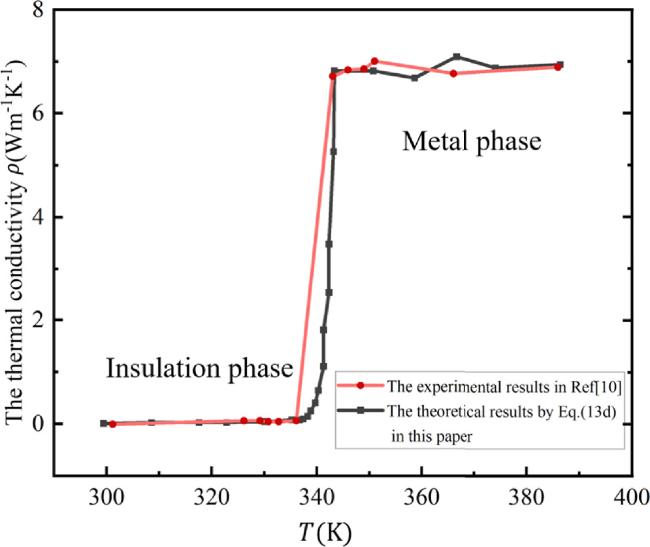
Figure 1. The thermal conductivity $\rho $ of vanadium dioxide calculated by the general WF law derived in equation ( |
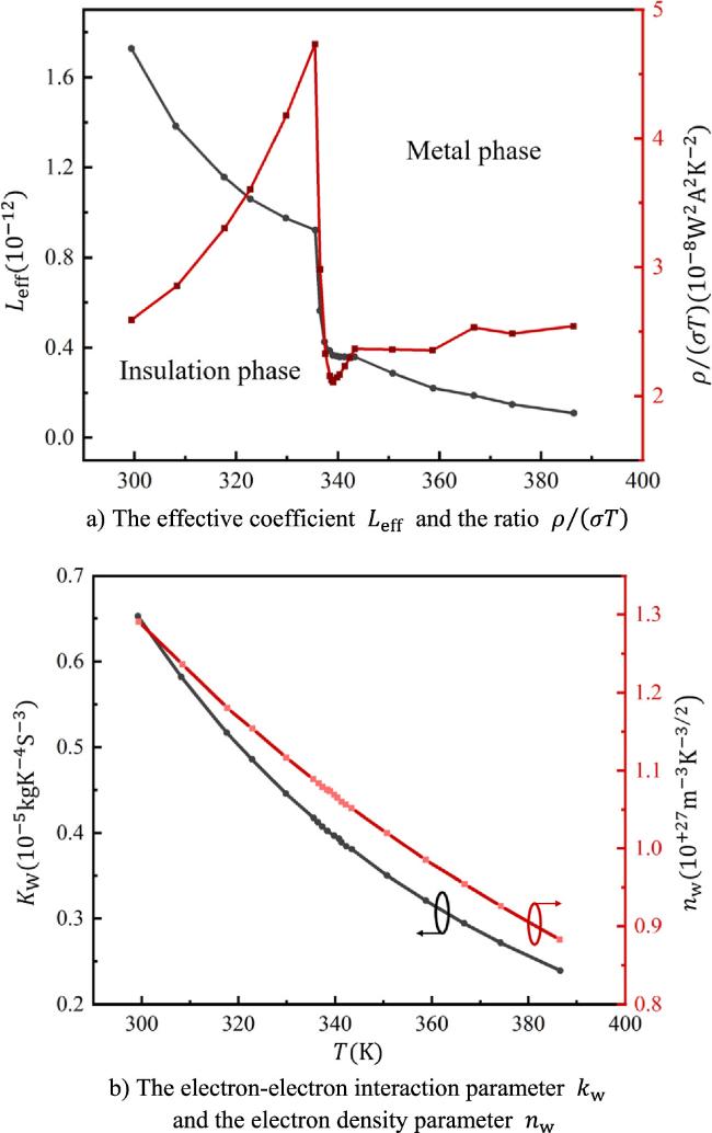
As shown in figure 1, in the electron transport process of vanadium dioxide, the thermal conductivity in the insulation phase caused by electron motion is less than one tenth of what WF law predicts. This was explained that the electrons are interrelated, which suppresses the randomness of the system, resulting in the extremely low electronic thermal conductivity of vanadium dioxide. To further explain this unusual low thermal conductivity, figure 2 shows the affection parameters in equation (13d ) for vanadium dioxide. From figure 2(a) it is found that the effective coefficient ${L}_{{\rm{eff}}}$ and the ratio $\rho /\left(\sigma T\right)$ in the insulation phase are both more than that in the metal phase. However, the electron-electron interaction parameter ${k}_{{\rm{w}}}\left(\propto {f}_{1}\left(\displaystyle \frac{\mu }{{k}_{{\rm{B}}}T}\right)\right)$ and the electron density parameter ${n}_{{\rm{w}}}$ $\left(\propto {f}_{2}\left(\displaystyle \frac{\mu }{{k}_{{\rm{B}}}T}\right)\right)$ are both decreased monotonically with temperature T, as shown in figure 2(b). Because in this insulation phase when T < 340 K, ${k}_{{\rm{w}}}$ and ${n}_{{\rm{w}}}$ are much more than the values in the metal phase when T > 340 K, this strongly correlated electron fluid causes independent diffusion of heat and charge, resulting in this unusual low thermal conductivity in the insulation phase.
Figure 2. The affection parameters in equation ( |
5. Conclusions
This paper presents a detailed derivation of a generalized WF law, employing the swallowtail catastrophe model and non-dimensional analysis. The derivation reveals that the relationship between thermal and electrical conductivity is fundamentally nonlinear, exhibiting a dependence on the relaxation time and chemical potential of the material. The resulting law satisfies the boundary conditions at both cryogenic and infinite-temperature limits. Furthermore, its validity is confirmed by the excellent agreement between our theoretical calculations for vanadium dioxide and previously reported experimental data.