


1. Introduction
Dispersive shock waves (DSWs) have been realized theoretically and experimentally in various hydrodynamic systems, including Bose–Einstein condensates [1–4], nonlinear optical systems [5–8], shallow water [9, 10] and plasma physics [11, 12]. As a nonlinear dynamic phenomenon, DSWs exhibit the characteristic formation of multivalued wavefronts in wave packets, with their structure well-represented by slowly modulated periodic phase waves [13]. Whitham modulation theory [14, 15] provides the simplest and most powerful framework for analyzing DSWs. This approach describes the slow evolution of nonlinear wave envelopes through the Whitham equations, which govern the spatiotemporal dynamics of all parameters characterizing a DSW. These equations are derived by averaging the conservation laws of the underlying wave equation over the rapid oscillations within the DSW. Researchers have developed multiple methods to derive the Whitham equations, notably the Lagrangian averaging method [16] and multi-scale perturbation method [17], which have greatly expanded modulation theory’s conceptual framework.
The Korteweg–de Vries (KdV) equation represents the first complete application of Whitham theory to integrable systems [13]. Since then, Whitham theory has been successfully extended to numerous other integrable systems [18], including the focusing and defocusing nonlinear Schrödinger (NLS) equation [19–23], the Kaup–Boussinesq equation [24], the derivative NLS (DNLS) equation [25], the defocusing complex modified KdV equation [26], the high-order Jaulent–Miodek equation [27], the Kundu equation [28], the Gerdjikov–Ivanov (GI) equation [29–31], the Gardner equation [32] and the cylindrical Gardner equation [33]. Over recent decades, Whitham modulation theory has experienced rapid development. Notably, the theory has been generalized to (2 + 1)-dimensional partial differential equations, enabling the study of (2 + 1)-dimensional DSWs in systems such as the Kadomtsev–Petviashvili equation [34] and the two-dimensional Benjamin–Ono equation [35].
The Kaup–Newell (KN) hierarchy is a physically and mathematically significant nonlinear system in soliton theory [36], encompassing the important nonlinear integrable equation known as the DNLS equation. Originally derived as a model for Alfvén waves propagating along the magnetic field in cold plasmas [37], the DNLS equation arises in disparate physical settings, including electromagnetic waves in an antiferromagnetic medium [38] and nonlinear asymmetric self-phase modulation and self-steepening of pulses in long optical waveguides [39, 40]. As the second-order flow in the KN hierarchy, the integrability by the inverse scattering transform method [36] and large classes of exact solutions have been studied extensively during the past decades [41, 42]. Reference [25] employed finite-gap integration and Whitham modulation theory to establish a complete classification of wave patterns arising from step-like initial conditions with arbitrary boundary conditions in the DNLS equation. The third-order KN equation, featuring third-order dispersion and quintic nonlinearity, was introduced by Kaup and Newell [36].
In this paper, we consider the following higher-order focusing KN model
$\begin{eqnarray}\begin{array}{r}{q}_{t}+{q}_{xxx}-3{\rm{i}}{\left(| q{| }^{2}{q}_{x}\right)}_{x}-\frac{3}{2}{\left(| q{| }^{4}q\right)}_{x}=0,\end{array}\end{eqnarray}$
which is the third-order flow equation of the KN hierarchy [36, 41, 42]. Furthermore, there exit another two kinds of third-order flow equation in the KN hierarchy, one is the third-order GI equation [31, 43–45] $\begin{eqnarray}\begin{array}{r}{q}_{t}+\frac{1}{2}{q}_{xxx}-\frac{3}{2}{\rm{i}}q{q}_{x}{q}_{x}^{* }+\frac{3}{4}| q{| }^{4}{q}_{x}=0,\end{array}\end{eqnarray}$
and the other one is the third-order Chen–Lee–Liu equation [46–48] $\begin{eqnarray}\begin{array}{r}{q}_{t}+{q}_{xxx}+\frac{3}{2}| q{| }^{2}{q}_{xx}-\frac{3}{4}| q{| }^{4}{q}_{x}+\frac{3}{2}{\rm{i}}{q}_{x}^{2}{q}^{* }=0.\end{array}\end{eqnarray}$
These higher-order models form a comprehensive theoretical framework for describing nonlinear wave evolution.Equation (1 ) is known to be integrable and exactly solvable via the inverse scattering transform [36]. Given that this model incorporates both third-order dispersion and quintic nonlinearity, it can effectively describe complex nonlinear phenomena in mathematical and physical systems. Previous studies using the Riemann–Hilbert approach have examined double and triple-pole solutions for equation (1 ) under both zero and non-zero boundary conditions [49]. Additionally, through Darboux transformation methods, various exact solutions including solitons, positons, breathers, and rogue waves have been obtained [50]. For the defocusing case of equation (1 ), the step-like initial value problem has been discussed based on Whitham modulation theory [51]. Compared with the defocusing case of equation (1 ), since the third term has an opposite sign, the wave structures exhibit different evolution dynamics in the focusing case. To the best of our knowledge, equation (1 ) remains relatively unexplored, particularly regarding the fundamental wave structures and a complete classification of the Riemann problem using Whitham modulation theory.
In many physical wave systems, the initial value problem under the hydrodynamic approximation is known to exhibit wave breaking in finite time. This behavior can be resolved by addressing the physical effects that originate from higher-order derivative terms in the evolution equations like equation (1 ) with third-order dispersion and quintic nonlinearity. Therefore, in this paper, we shall derive the Whitham equations which govern the slow evolution of a nonlinear periodic wave arising from the discontinuous initial-value conditions. We shall discuss the solution classification of the Riemann problem of equation (1 ) and present many exotic undular bores. These findings not only deepen the fundamental understanding of physical processes such as optical wave breaking and pulse splitting, but also provide a theoretical foundation for optimizing practical applications including ultrafast laser technologies and advanced optical communication systems.
The remainder of this paper is organized as follows. In section 2 , we employ the finite-gap integration method to derive periodic solutions and establish the corresponding Whitham modulation equations. Section 3 presents the elementary wave structures emerging from initial discontinuities. A complete classification of solutions for the step-like initial value problem is provided in section 4 . Finally, we summarize our results and present concluding remarks in section 5 .
2. Periodic solutions and Whitham modulation equations
Equation (1 ) has the following Lax pair 1 ).
$\begin{eqnarray}\begin{array}{r}{{\rm{\Psi }}}_{x}=\left(\begin{array}{cc}F & G\\ H & -F\end{array}\right){\rm{\Psi }},\qquad {{\rm{\Psi }}}_{t}=\left(\begin{array}{cc}A & B\\ C & -A\end{array}\right){\rm{\Psi }},\end{array}\end{eqnarray}$
with $\begin{eqnarray*}\begin{array}{rcl}F & = & {\rm{i}}{\lambda }^{2},\,G=q\lambda ,\,H=-{q}^{* }\lambda ,\\ A & = & 4{\rm{i}}{\lambda }^{6}+\frac{3}{2}{\rm{i}}| q{| }^{4}{\lambda }^{2}-2{\rm{i}}| q{| }^{2}{\lambda }^{4}+q{q}_{x}^{* }{\lambda }^{2}-{q}_{x}{q}^{* }{\lambda }^{2},\\ B & = & 4q{\lambda }^{5}+\frac{3}{2}| q{| }^{4}q\lambda -2| q{| }^{2}q{\lambda }^{3}-2{\rm{i}}{q}_{x}{\lambda }^{3}\\ & & +3{\rm{i}}| q{| }^{2}{q}_{x}\lambda -{q}_{xx}\lambda ,\\ C & = & -4{q}^{* }{\lambda }^{5}-\frac{3}{2}| q{| }^{4}{q}^{* }\lambda +2| q{| }^{2}{q}^{* }{\lambda }^{3}-2{\rm{i}}{q}_{x}^{* }{\lambda }^{3}\\ & & +3{\rm{i}}| q{| }^{2}{q}_{x}^{* }\lambda -{q}_{xx}^{* }\lambda ,\end{array}\end{eqnarray*}$
where $\Psi$ is the vector eigenfunction and λ is the spectral parameter. It can be checked that the compatibility condition $\Psi$xt = $\Psi$tx can yield equation (We assume that (φ1, φ2) and (Φ1, Φ2) are two linearly independent fundamental solution of the Lax pair (4 ), and define the squared wave functions
$\begin{eqnarray}\begin{array}{r}f=-\frac{{\rm{i}}}{2}\left({\psi }_{1}{\phi }_{2}+{\psi }_{2}{\phi }_{1}\right),\,g={\psi }_{1}{\phi }_{1},\,h=-{\psi }_{2}{\phi }_{2},\end{array}\end{eqnarray}$
where f, g and h satisfy the following linear system $\begin{eqnarray}\begin{array}{rcl}{f}_{x} & = & -{\rm{i}}Hg+{\rm{i}}Gh,\,{g}_{x}=2{\rm{i}}Gf+2Fg,\\ {h}_{x} & = & -2{\rm{i}}Hf-2Fh,\end{array}\end{eqnarray}$
$\begin{eqnarray}\begin{array}{rcl}{f}_{t} & = & -{\rm{i}}Cg+{\rm{i}}Bh,\,\,{g}_{t}=2{\rm{i}}Bf+2Ag,\\ {h}_{t} & = & -2{\rm{i}}Cf-2Ah.\end{array}\end{eqnarray}$
It is easy to verify that the Wronskian φ1Φ2 − φ2Φ1 is independent of x and t. Therefore, ${f}^{2}-gh=-\frac{1}{4}{\left({\psi }_{1}{\phi }_{2}-{\psi }_{2}{\phi }_{1}\right)}^{2}$ is an integral of motion depending only the spectral parameter λ. It is known that the periodic solutions of evolution equations are determined by the the condition that P(λ) = f2 − gh must be a polynomial in λ.To derive the Whitham modulation equations for equation (1 ), we first construct the conservation equation from linear system (6 ) and (7 ). The second equation in each of linear system (6 ) and (7 ) can be reformulated as 1 ) can be derived from the following equation
$\begin{eqnarray}\begin{array}{rcl}{\left(\mathrm{log}g\right)}_{x} & = & \frac{{g}_{x}}{g}=2{\rm{i}}\,f\frac{G}{g}+2F,\\ {\left(\mathrm{log}g\right)}_{t} & = & \frac{{g}_{t}}{g}=2{\rm{i}}\,f\frac{B}{g}+2A.\end{array}\end{eqnarray}$
Therefore, by use of the equality ${(\mathrm{log}g)}_{xt}={(\mathrm{log}g)}_{tx}$, the conservation laws of equation ( $\begin{eqnarray}\begin{array}{r}\frac{\partial }{\partial t}\left(\frac{G}{g}\right)=\frac{\partial }{\partial x}\left(\frac{B}{g}\right).\end{array}\end{eqnarray}$
To obtain the periodic solution of equation (1 ), the polynomial $P\left(\lambda \right)$ can be expressed by 10 )
$\begin{eqnarray}\begin{array}{rcl}P\left(\lambda \right) & = & {f}^{2}-gh=\displaystyle \prod _{i=1}^{4}\left({\lambda }^{2}-{\lambda }_{i}^{2}\right)\\ & = & {\lambda }^{8}-{s}_{1}{\lambda }^{6}+{s}_{2}{\lambda }^{4}-{s}_{3}{\lambda }^{2}+{s}_{4}.\end{array}\end{eqnarray}$
According to the root-solving formula, the relationship between the coefficients si and the roots ${\lambda }_{i}^{2}$ $\left(i=1,2,3,4\right)$ can be explicitly established through the polynomial ( $\begin{eqnarray}\begin{array}{r}{s}_{1}={\lambda }_{1}^{2}+{\lambda }_{2}^{2}+{\lambda }_{3}^{2}+{\lambda }_{4}^{2},\end{array}\end{eqnarray}$
$\begin{eqnarray}\begin{array}{rcl}{s}_{2} & = & {\lambda }_{1}^{2}{\lambda }_{2}^{2}+{\lambda }_{1}^{2}{\lambda }_{3}^{2}+{\lambda }_{1}^{2}{\lambda }_{4}^{2}\\ & & +{\lambda }_{2}^{2}{\lambda }_{3}^{2}+{\lambda }_{2}^{2}{\lambda }_{4}^{2}+{\lambda }_{3}^{2}{\lambda }_{4}^{2},\end{array}\end{eqnarray}$
$\begin{eqnarray}\begin{array}{r}{s}_{3}={\lambda }_{1}^{2}{\lambda }_{2}^{2}{\lambda }_{3}^{2}+{\lambda }_{1}^{2}{\lambda }_{2}^{2}{\lambda }_{4}^{2}+{\lambda }_{1}^{2}{\lambda }_{3}^{2}{\lambda }_{4}^{2}+{\lambda }_{2}^{2}{\lambda }_{3}^{2}{\lambda }_{4}^{2},\end{array}\end{eqnarray}$
$\begin{eqnarray}\begin{array}{r}{s}_{4}={\lambda }_{1}^{2}{\lambda }_{2}^{2}{\lambda }_{3}^{2}{\lambda }_{4}^{2}.\end{array}\end{eqnarray}$
The polynomials f, g and h, expressed in terms of the spectral parameter λ, take the following explicit forms: 15 ) into equations (6 ) and (7 ) yields
$\begin{eqnarray}\begin{array}{rcl}f\left(x,t,\lambda \right) & = & -{\lambda }^{4}+{f}_{1}{\lambda }^{2}-{f}_{2},\,g\left(x,t,\lambda \right)\\ & = & \lambda \left({\lambda }^{2}-\mu \right)q,\,h\left(x,t,\lambda \right)=-\lambda \left({\lambda }^{2}-{\mu }^{* }\right){q}^{* }.\end{array}\end{eqnarray}$
Substituting equation ( $\begin{eqnarray}\begin{array}{r}{f}_{2x}=0,\,{f}_{1x}={\rm{i}}| q{| }^{2}\left({\mu }^{* }-\mu \right),\end{array}\end{eqnarray}$
$\begin{eqnarray}\begin{array}{r}{q}_{x}=2{\rm{i}}q\left({f}_{1}-\mu \right),\,| q{| }_{x}^{2}=2{\rm{i}}| q{| }^{2}\left({\mu }^{* }-\mu \right),\end{array}\end{eqnarray}$
$\begin{eqnarray}\begin{array}{r}{\mu }_{x}=2{\rm{i}}\left({\mu }^{2}-{f}_{1}\mu +{f}_{2}\right),\end{array}\end{eqnarray}$
and $\begin{eqnarray}\begin{array}{rcl}{f}_{2t}=0,\,{f}_{1t} & = & \frac{1}{2}{\rm{i}}| q{| }^{2}\left({\mu }^{* }-\mu \right)\left(8{f}_{1}^{2}-8{f}_{2}\right.\\ & & \left.-12{f}_{1}| q{| }^{2}+4\mu | q{| }^{2}+4{\mu }^{* }| q{| }^{2}+3| q{| }^{4}\right),\end{array}\end{eqnarray}$
$\begin{eqnarray}\begin{array}{rcl}{q}_{t} & = & 8{\rm{i}}q\left({f}_{1}^{3}-2{f}_{1}{f}_{2}-\mu {f}_{1}^{2}+\mu {f}_{2}\right)\\ & & -4{\rm{i}}| q{| }^{2}q\left(3{f}_{1}^{2}-{f}_{2}-4\mu {f}_{1}+{\mu }^{2}\right)\\ & & +3{\rm{i}}| q{| }^{4}q\left({f}_{1}-\mu \right)+4{\rm{i}}| q{| }^{2}q{\mu }^{* }\left({f}_{1}-\mu \right),\end{array}\end{eqnarray}$
$\begin{eqnarray}\begin{array}{rcl}| q{| }_{t}^{2} & = & {\rm{i}}| q{| }^{2}\left({\mu }^{* }-\mu \right)\\ & & \times \left[8{f}_{1}^{2}-8{f}_{2}-4| q{| }^{2}\left(3{f}_{1}-\mu -{\mu }^{* }\right)+3| q{| }^{4}\right],\end{array}\end{eqnarray}$
$\begin{eqnarray}\begin{array}{l}{\mu }_{t}=-{\rm{i}}\left[{f}_{2}+\mu \left(\mu -{f}_{1}\right)\right]\\ \unicode{8199}\unicode{8199}\unicode{8199}\unicode{8199}\times \left[-8{f}_{1}^{2}+8{f}_{2}+12{f}_{2}| q{| }^{2}-| q{| }^{2}\left(4\mu +3| q{| }^{2}+4{\mu }^{* }\right)\right].\end{array}\end{eqnarray}$
By substituting equation (15 ) into equation (10 ) and comparing the coefficients of the powers of λ, we can further derive the following relations: 28 ). For the case ${f}_{2}=-\sqrt{{s}_{4}}$, the zeroes 28 ). In both cases, under the assumption of the ordering 0 ≥ λ1 ≥ λ2 ≥ λ3 ≥ λ4, it is straightforward to deduce that ρ1 ≥ ρ2 ≥ ρ3 ≥ ρ4.
$\begin{eqnarray}\begin{array}{r}{s}_{1}=2{f}_{1}-\rho ,\,{s}_{2}={f}_{1}^{2}+2{f}_{2}-\rho \mu -\rho {\mu }^{* },\end{array}\end{eqnarray}$
$\begin{eqnarray}\begin{array}{r}{s}_{3}=2{f}_{1}{f}_{2}-\rho \mu {\mu }^{* },\,{s}_{4}={f}_{2}^{2},\end{array}\end{eqnarray}$
which indicate that $\begin{eqnarray}\begin{array}{r}{f}_{1}=\frac{{s}_{1}+\rho }{2},\,{f}_{2}=\pm \sqrt{{s}_{4}},\end{array}\end{eqnarray}$
$\begin{eqnarray}\begin{array}{r}\mu =\frac{1}{8\rho }\left[{\left({s}_{1}+\rho \right)}^{2}\pm 8\sqrt{{s}_{4}}-4{s}_{2}-{\rm{i}}\sqrt{-R\left(\rho \right)}\right],\end{array}\end{eqnarray}$
$\begin{eqnarray}\begin{array}{r}{\mu }^{* }=\frac{1}{8\rho }\left[{\left({s}_{1}+\rho \right)}^{2}\pm 8\sqrt{{s}_{4}}-4{s}_{2}+{\rm{i}}\sqrt{-R\left(\rho \right)}\right],\end{array}\end{eqnarray}$
where $\begin{eqnarray}\begin{array}{rcl}R(\rho ) & = & {\rho }^{4}+4{s}_{1}{\rho }^{3}+\left(6{s}_{1}^{2}-8{s}_{2}\mp 48\sqrt{{s}_{4}}\right){\rho }^{2}\\ & & +\left(4{s}_{1}^{3}-16{s}_{1}{s}_{2}+64{s}_{3}\mp 32{s}_{1}\sqrt{{s}_{4}}\right)\rho \\ & & +{\left({s}_{1}^{2}-4{s}_{2}\pm 8\sqrt{{s}_{4}}\right)}^{2}.\end{array}\end{eqnarray}$
The zeroes of the polynomial R(ρ) are connected to the zeroes of P(λ). For the case ${f}_{2}=\sqrt{{s}_{4}}$, the zeroes of the polynomial R(ρ) $\begin{eqnarray}\begin{array}{rcl}{\rho }_{1} & = & -{\left({\lambda }_{1}-{\lambda }_{2}-{\lambda }_{3}+{\lambda }_{4}\right)}^{2},\\ {\rho }_{2} & = & -{\left({\lambda }_{1}-{\lambda }_{2}+{\lambda }_{3}-{\lambda }_{4}\right)}^{2},\\ {\rho }_{3} & = & -{\left({\lambda }_{1}+{\lambda }_{2}-{\lambda }_{3}-{\lambda }_{4}\right)}^{2},\\ {\rho }_{4} & = & -{\left({\lambda }_{1}+{\lambda }_{2}+{\lambda }_{3}+{\lambda }_{4}\right)}^{2},\end{array}\end{eqnarray}$
correspond to the upper sign in equation ( $\begin{eqnarray}\begin{array}{rcl}{\rho }_{1} & = & -{\left({\lambda }_{1}+{\lambda }_{2}+{\lambda }_{3}-{\lambda }_{4}\right)}^{2},\\ {\rho }_{2} & = & -{\left({\lambda }_{1}+{\lambda }_{2}-{\lambda }_{3}+{\lambda }_{4}\right)}^{2},\\ {\rho }_{3} & = & -{\left({\lambda }_{1}-{\lambda }_{2}+{\lambda }_{3}+{\lambda }_{4}\right)}^{2},\\ {\rho }_{4} & = & -{\left({\lambda }_{1}-{\lambda }_{2}-{\lambda }_{3}-{\lambda }_{4}\right)}^{2},\end{array}\end{eqnarray}$
correspond to the lower sign in equation (Using equations (25 )−(27 ), ρx and ρt can be concluded that 32 ), it is understood that the function ρ oscillates within one of the two possible intervals ρ4 ≤ ρ ≤ ρ3 and ρ2 ≤ ρ ≤ ρ2 (see Figure 1).
$\begin{eqnarray}\begin{array}{r}{\rho }_{x}=2{\rm{i}}\rho \left({\mu }^{* }-\mu \right)=\frac{1}{2}\sqrt{-R\left(\rho \right)},\,{\rho }_{t}={\rho }_{x}\left(\frac{3}{2}{s}_{1}^{2}-2{s}_{2}\right),\end{array}\end{eqnarray}$
which indicate ρ depends on the phase ξ = x − Vt$(V=2{s}_{2}-\frac{3}{2}{s}_{1}^{2})$ only $\begin{eqnarray}\begin{array}{r}\frac{{\rm{d}}\rho }{{\rm{d}}\xi }=\frac{1}{2}\sqrt{-R\left(\rho \right)}.\end{array}\end{eqnarray}$
From equations (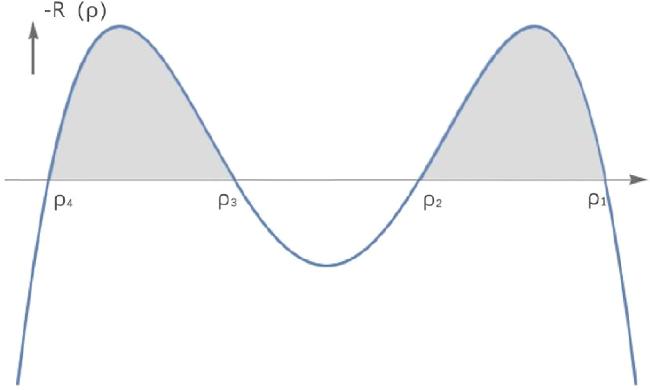
Figure 1. The ‘Potential’ curve −R(ρ) configurations of the third-order focusing Kaup–Newell model. |
For the case ρ4 ≤ ρ ≤ ρ3, the periodic wave solution of equation (32 ) can be expressed by the Jacobi elliptic function 33 ) degenerates into
$\begin{eqnarray}\begin{array}{r}\rho =\frac{{\rho }_{4}\left({\rho }_{1}-{\rho }_{3}\right)+{\rho }_{1}\left({\rho }_{3}-{\rho }_{4}\right){{\rm{sn}}}^{2}\left(\theta ,m\right)}{{\rho }_{1}-{\rho }_{3}+\left({\rho }_{3}-{\rho }_{4}\right){{\rm{sn}}}^{2}\left(\theta ,m\right)},\end{array}\end{eqnarray}$
with $\begin{eqnarray}\begin{array}{r}\theta =\frac{1}{4}\sqrt{\left({\rho }_{1}-{\rho }_{3}\right)\left({\rho }_{2}-{\rho }_{4}\right)}\xi ,\,m=\frac{\left({\rho }_{3}-{\rho }_{4}\right)\left({\rho }_{2}-{\rho }_{1}\right)}{\left({\rho }_{3}-{\rho }_{1}\right)\left({\rho }_{2}-{\rho }_{4}\right)},\end{array}\end{eqnarray}$
where m is the modulus of the Jacobi elliptic sn function. The wavelength L of the periodic wave is given by $\begin{eqnarray}\begin{array}{r}L=\frac{8K\left(m\right)}{\sqrt{\left({\rho }_{1}-{\rho }_{3}\right)\left({\rho }_{2}-{\rho }_{4}\right)}},\end{array}\end{eqnarray}$
where K(m) is the complete elliptic integral of the first kind. In the limit m → 1(i.e. ρ2 → ρ3), the periodic solution ( $\begin{eqnarray}\begin{array}{r}\rho =\frac{{\rho }_{4}\left({\rho }_{1}-{\rho }_{3}\right)+{\rho }_{1}\left({\rho }_{3}-{\rho }_{4}\right){{\rm{\tanh }}}^{2}\left({\theta }_{0}\right)}{{\rho }_{1}-{\rho }_{3}+\left({\rho }_{3}-{\rho }_{4}\right){{\rm{\tanh }}}^{2}\left({\theta }_{0}\right)},\end{array}\end{eqnarray}$
where ${\theta }_{0}=\frac{1}{4}\sqrt{\left({\rho }_{1}-{\rho }_{3}\right)\left({\rho }_{3}-{\rho }_{4}\right)}\xi $.In the limit m → 0, two distinct scenarios emerge: ρ1 → ρ2 and ρ3 → ρ4. For the case ρ1 → ρ2, the periodic solution (33 ) degenerates into a trigonometric wave solution
$\begin{eqnarray}\begin{array}{r}\rho =\frac{{\rho }_{3}\left({\rho }_{2}-{\rho }_{4}\right)-{\rho }_{2}\left({\rho }_{3}-{\rho }_{4}\right){{\rm{\cos }}}^{2}\left({\theta }_{1}\right)}{{\rho }_{2}-{\rho }_{3}+\left({\rho }_{3}-{\rho }_{4}\right){{\rm{\sin }}}^{2}\left({\theta }_{1}\right)},\end{array}\end{eqnarray}$
where ${\theta }_{1}=\frac{1}{4}\sqrt{\left({\rho }_{2}-{\rho }_{3}\right)\left({\rho }_{2}-{\rho }_{4}\right)}\xi $.For the case ρ3 → ρ4, the periodic solution (33 ) degenerates into a constant solution ρ = ρ3.
Similarly, for ρ2 ≤ ρ ≤ ρ1, the periodic wave solution of equations (32 ) can be expressed by the Jacobi elliptic function 34 ).
$\begin{eqnarray}\begin{array}{r}\rho =\frac{{\rho }_{1}\left({\rho }_{4}-{\rho }_{2}\right)+{\rho }_{4}\left({\rho }_{2}-{\rho }_{1}\right){{\rm{sn}}}^{2}\left(\theta ,m\right)}{{\rho }_{4}-{\rho }_{2}+\left({\rho }_{2}-{\rho }_{1}\right){{\rm{sn}}}^{2}\left(\theta ,m\right)},\end{array}\end{eqnarray}$
with the same definitions for θ and m in equations (In the limit m → 1(i.e. ρ2 → ρ3), the periodic solution (38 ) degenerates into
$\begin{eqnarray}\begin{array}{r}\rho =\frac{{\rho }_{2}\left({\rho }_{4}-{\rho }_{1}\right)-{\rho }_{4}\left({\rho }_{2}-{\rho }_{1}\right){{\rm{{\rm{sech}} }}}^{2}\left({\theta }_{0}\right)}{{\rho }_{4}-{\rho }_{1}+\left({\rho }_{1}-{\rho }_{2}\right){{\rm{{\rm{sech}} }}}^{2}\left({\theta }_{0}\right)},\end{array}\end{eqnarray}$
where ${\theta }_{0}=\frac{1}{4}\sqrt{\left({\rho }_{1}-{\rho }_{3}\right)\left({\rho }_{3}-{\rho }_{4}\right)}\xi $.In the limit m → 0, two distinct scenarios emerge: ρ1 → ρ2 and ρ3 → ρ4. For the case of ρ1 → ρ2, the periodic solution (38 ) degenerates into a constant solution ρ = ρ2. While ρ3 → ρ4, the periodic solution (33 ) degenerates into a trigonometric wave solution
$\begin{eqnarray}\begin{array}{r}\rho =\frac{{\rho }_{2}\left({\rho }_{4}-{\rho }_{1}\right)+{\rho }_{4}\left({\rho }_{1}-{\rho }_{2}\right){{\rm{\cos }}}^{2}\left({\theta }_{2}\right)}{{\rho }_{4}-{\rho }_{2}+\left({\rho }_{2}-{\rho }_{1}\right){{\rm{\sin }}}^{2}\left({\theta }_{2}\right)},\end{array}\end{eqnarray}$
where ${\theta }_{2}=\frac{1}{4}\sqrt{\left({\rho }_{1}-{\rho }_{4}\right)\left({\rho }_{2}-{\rho }_{4}\right)}\xi $.In the following, we need to construct the Whitham equations for the periodic solution. By transforming $g\to g/\sqrt{P\left(\lambda \right)}$, the conservation law equation (9 ) becomes 4 ) and (15 ) into equation (41 ) gives 42 ) over the wavelength 1 ) for Riemann invariant ${\lambda }_{i}\left(i=1,2,3,4\right)$ are derived as follows 47 ) and (48 ), the Whitham velocities ${v}_{i}={v}_{i}\left({\lambda }_{i}\right)$ can be written as
$\begin{eqnarray}\begin{array}{r}\frac{\partial }{\partial t}\left(\frac{G\sqrt{P\left(\lambda \right)}}{g}\right)-\frac{\partial }{\partial x}\left(\frac{B\sqrt{P\left(\lambda \right)}}{g}\right)=0.\end{array}\end{eqnarray}$
Then, substitution of equations ( $\begin{eqnarray}\begin{array}{r}\begin{array}{l}\frac{\partial }{\partial t}\left(\frac{\sqrt{P\left(\lambda \right)}}{{\lambda }^{2}-\mu }\right)\\ \quad -\frac{\partial }{\partial x}\left[\sqrt{P\left(\lambda \right)}\left(4{\lambda }^{2}+2{s}_{1}+\frac{\frac{3}{2}{s}_{1}^{2}-2{s}_{2}}{{\lambda }^{2}-\mu }\right)\right]=0.\end{array}\end{array}\end{eqnarray}$
By averaging of equation ( $\begin{eqnarray}\begin{array}{r}L=\oint \frac{{\rm{d}}\mu }{2\sqrt{-P\left({\mu }^{1/2}\right)}},\end{array}\end{eqnarray}$
we obtain the averaged conservation law $\begin{eqnarray*}\begin{array}{l}\frac{\partial }{\partial t}\left(\frac{\sqrt{P\left(\lambda \right)}}{L}\oint \frac{{\rm{d}}\mu }{2\left({\lambda }^{2}-\mu \right)\sqrt{-P\left({\mu }^{1/2}\right)}}\right)-\frac{\partial }{\partial x}\left[\Space{0ex}{4.25ex}{0ex}\sqrt{P\left(\lambda \right)}\left(4{\lambda }^{2}\right.\right.\\ +\left.\left.2{s}_{1}+\frac{\frac{3}{2}{s}_{1}^{2}-2{s}_{2}}{L}\oint \frac{{\rm{d}}\mu }{2\left({\lambda }^{2}-\mu \right)\sqrt{-P\left({\mu }^{1/2}\right)}}\right)\right]=0.\end{array}\end{eqnarray*}$
Expanding the above equation and taking the limit λ → λi(i = 1, 2, 3, 4), we obtain $\begin{eqnarray}\begin{array}{l}\oint \frac{{\rm{d}}\mu }{2\left({\lambda }_{i}^{2}-\mu \right)\sqrt{-P\left({\mu }^{1/2}\right)}}\frac{\partial {\lambda }_{i}^{2}}{\partial t}-\left[\Space{0ex}{3.75ex}{0ex}\left(4{\lambda }_{i}^{2}+2{s}_{1}\right)L\right.\\ \left.+\left(\frac{3}{2}{s}_{1}-2{s}_{2}\right)\oint \frac{{\rm{d}}\mu }{2\left({\lambda }_{i}^{2}-\mu \right)\sqrt{-P\left({\mu }^{1/2}\right)}}\right]\frac{\partial {\lambda }_{i}^{2}}{\partial x}=0.\end{array}\end{eqnarray}$
Consequently, the Whitham modulation equations of equation ( $\begin{eqnarray}\begin{array}{r}\frac{\partial {\lambda }_{i}^{2}}{\partial t}+{v}_{i}\left({\lambda }_{i}\right)\frac{\partial {\lambda }_{i}^{2}}{\partial x}=0,\end{array}\end{eqnarray}$
with the Whitham velocities $\begin{eqnarray}\begin{array}{r}{v}_{i}=-\frac{{I}_{2}\left({\lambda }_{i}\right)}{{I}_{1}\left({\lambda }_{i}\right)},\end{array}\end{eqnarray}$
where ${I}_{1}={I}_{1}\left({\lambda }_{i}\right)$ and ${I}_{2}={I}_{2}\left({\lambda }_{i}\right)$ represent $\begin{eqnarray}\begin{array}{r}{I}_{1}=\oint \frac{{\rm{d}}\mu }{\left(2{\lambda }_{i}^{2}-\mu \right)\sqrt{-P\left({\mu }^{1/2}\right)}},\end{array}\end{eqnarray}$
$\begin{eqnarray}\begin{array}{rcl}{I}_{2} & = & \left(4{\lambda }_{i}^{2}+2{s}_{1}\right)L+\left(\frac{3}{2}{s}_{1}-2{s}_{2}\right)\\ & & \times \oint \frac{{\rm{d}}\mu }{2\left({\lambda }_{i}^{2}-\mu \right)\sqrt{-P\left({\mu }^{1/2}\right)}}\\ & = & \left(4{\lambda }_{i}^{2}+2{s}_{1}\right)L+\left(\frac{3}{2}{s}_{1}-2{s}_{2}\right){I}_{1}.\end{array}\end{eqnarray}$
According to equations ( $\begin{eqnarray}\begin{array}{r}{v}_{i}=V+\frac{\left(2{\lambda }_{i}^{2}+{s}_{1}\right)L}{\partial L/\partial {\lambda }_{i}^{2}},\,(i=1,2,3,4).\end{array}\end{eqnarray}$
We define the new Riemann invariants ri by the formula 29 ) and (30 ) are expressed in terms of ri as 45 ) for the Riemann invariants ${r}_{i}\left(i=1,2,3,4\right)$ can be rewritten as
$\begin{eqnarray}\begin{array}{r}{r}_{i}=-{\lambda }_{i}^{2},\,(i=1,2,3,4),\end{array}\end{eqnarray}$
which are ordered according to 0 ≥ r1 ≥ r2 ≥ r3 ≥ r4 for 0 ≥ λ1 ≥ λ2 ≥ λ3 ≥ λ4. Therefore, the parameters ρi in equations ( $\begin{eqnarray}\begin{array}{rcl}{\rho }_{1} & = & -{(\sqrt{-{r}_{1}}-\sqrt{-{r}_{2}}-\sqrt{-{r}_{3}}+\sqrt{-{r}_{4}})}^{2},\\ {\rho }_{2} & = & -{(-\sqrt{{r}_{1}}-\sqrt{-{r}_{2}}+\sqrt{-{r}_{3}}-\sqrt{-{r}_{4}})}^{2},\\ {\rho }_{3} & = & -{(\sqrt{-{r}_{1}}+\sqrt{-{r}_{2}}-\sqrt{-{r}_{3}}-\sqrt{-{r}_{4}})}^{2},\\ {\rho }_{4} & = & -{(\sqrt{-{r}_{1}}+\sqrt{-{r}_{2}}+\sqrt{-{r}_{3}}+\sqrt{-{r}_{4}})}^{2},\end{array}\end{eqnarray}$
and $\begin{eqnarray}\begin{array}{rcl}{\rho }_{1} & = & -{(\sqrt{-{r}_{1}}+\sqrt{-{r}_{2}}+\sqrt{-{r}_{3}}-\sqrt{-{r}_{4}})}^{2},\\ {\rho }_{2} & = & -{(\sqrt{-{r}_{1}}+\sqrt{-{r}_{2}}-\sqrt{-{r}_{3}}+\sqrt{-{r}_{4}})}^{2},\\ {\rho }_{3} & = & -{(\sqrt{-{r}_{1}}-\sqrt{-{r}_{2}}+\sqrt{-{r}_{3}}+\sqrt{-{r}_{4}})}^{2},\\ {\rho }_{4} & = & -{(\sqrt{-{r}_{1}}-\sqrt{-{r}_{2}}-\sqrt{-{r}_{3}}-\sqrt{-{r}_{4}})}^{2}.\end{array}\end{eqnarray}$
In this case, the phase velocity V, the wavelength L and the modulus m can be rewritten as $\begin{eqnarray}\begin{array}{rcl}V & = & 2\displaystyle \sum _{i\lt j}^{4}{r}_{i}{r}_{j}-\frac{3}{2}{\left(\displaystyle \sum _{i=1}^{4}{r}_{i}\right)}^{2},\\ L & = & \frac{2K\left(m\right)}{\sqrt{\left({r}_{1}-{r}_{3}\right)\left({r}_{2}-{r}_{4}\right)}},\\ m & = & \frac{\left({r}_{1}-{r}_{2}\right)\left({r}_{3}-{r}_{4}\right)}{\left({r}_{1}-{r}_{3}\right)\left({r}_{2}-{r}_{4}\right)}.\end{array}\end{eqnarray}$
In addition, the Whitham modulation equation ( $\begin{eqnarray}\begin{array}{r}\frac{\partial {r}_{i}}{\partial t}+{v}_{i}\left({r}_{i}\right)\frac{\partial {r}_{i}}{\partial x}=0,\,(i=1,2,3,4),\end{array}\end{eqnarray}$
where the Whitham velocities ${v}_{i}={v}_{i}\left({r}_{i}\right)\left(i=1,2,3,4\right)$ are $\begin{eqnarray}\begin{array}{r}{v}_{i}=V+\frac{\left(2{r}_{i}-{s}_{1}\right)L}{\partial L/\partial {r}_{i}},\,(i=1,2,3,4)\end{array}\end{eqnarray}$
with the characteristic velocities $\begin{eqnarray}\begin{array}{rcl}{v}_{1} & = & 2\displaystyle \sum _{i\lt j}^{4}{r}_{i}{r}_{j}-\frac{3}{2}{\left(\displaystyle \sum _{i=1}^{4}{r}_{i}\right)}^{2}\\ & & +\frac{2\left({r}_{1}-{r}_{2}\right)\left({r}_{1}-{r}_{4}\right)\left(3{r}_{1}+{r}_{2}+{r}_{3}+{r}_{4}\right)K\left(m\right)}{\left({r}_{2}-{r}_{4}\right)E\left(m\right)+\left({r}_{4}-{r}_{1}\right)K\left(m\right)},\end{array}\end{eqnarray}$
$\begin{eqnarray}\begin{array}{rcl}{v}_{2} & = & 2\displaystyle \sum _{i\lt j}^{4}{r}_{i}{r}_{j}-\frac{3}{2}{\left(\displaystyle \sum _{i=1}^{4}{r}_{i}\right)}^{2}\\ & & +\frac{2\left({r}_{1}-{r}_{2}\right)\left({r}_{3}-{r}_{2}\right)\left({r}_{1}+3{r}_{2}+{r}_{3}+{r}_{4}\right)K\left(m\right)}{\left({r}_{1}-{r}_{3}\right)E\left(m\right)+\left({r}_{3}-{r}_{2}\right)K\left(m\right)},\end{array}\end{eqnarray}$
$\begin{eqnarray}\begin{array}{rcl}{v}_{3} & = & 2\displaystyle \sum _{i\lt j}^{4}{r}_{i}{r}_{j}-\frac{3}{2}{\left(\displaystyle \sum _{i=1}^{4}{r}_{i}\right)}^{2}\\ & & +\frac{2\left({r}_{3}-{r}_{2}\right)\left({r}_{3}-{r}_{4}\right)\left({r}_{1}+{r}_{2}+3{r}_{3}+{r}_{4}\right)K\left(m\right)}{\left({r}_{4}-{r}_{2}\right)E\left(m\right)+\left({r}_{2}-{r}_{3}\right)K\left(m\right)},\end{array}\end{eqnarray}$
$\begin{eqnarray}\begin{array}{rcl}{v}_{4} & = & 2\displaystyle \sum _{i\lt j}^{4}{r}_{i}{r}_{j}-\frac{3}{2}{\left(\displaystyle \sum _{i=1}^{4}{r}_{i}\right)}^{2}\\ & & +\frac{2\left({r}_{1}-{r}_{4}\right)\left({r}_{3}-{r}_{4}\right)\left({r}_{1}+{r}_{2}+{r}_{3}+3{r}_{4}\right)K\left(m\right)}{\left({r}_{3}-{r}_{1}\right)E\left(m\right)+\left({r}_{1}-{r}_{4}\right)K\left(m\right)},\end{array}\end{eqnarray}$
where $E\left(m\right)$ is the second kind complete elliptic integral.In the small amplitude limit m → 0, this limit corresponds to two cases. For the limit state r1 → r2, the Whitham velocities ${v}_{i}\left(i=1,2,3,4\right)$ degenerate into
$\begin{eqnarray}\begin{array}{l}{v}_{1}={v}_{2}\\ =\frac{-48{r}_{1}^{3}+6{r}_{1}{\left({r}_{3}-{r}_{4}\right)}^{2}+24{r}_{1}^{2}\left({r}_{3}+{r}_{4}\right)+3{\left({r}_{3}-{r}_{4}\right)}^{2}\left({r}_{3}+{r}_{4}\right)}{2\left(2{r}_{1}-{r}_{3}-{r}_{4}\right)},\\ {v}_{3}=-\frac{3}{2}\left(5{r}_{3}^{2}+2{r}_{3}{r}_{4}+{r}_{4}^{2}\right),\\ {v}_{4}=-\frac{3}{2}\left({r}_{3}^{2}+2{r}_{3}{r}_{4}+5{r}_{4}^{2}\right),\end{array}\end{eqnarray}$
and the limit state r3 → r4 can be reduced to $\begin{eqnarray}\begin{array}{l}{v}_{1}=-\frac{3}{2}\left(5{r}_{1}^{2}+2{r}_{1}{r}_{2}+{r}_{2}^{2}\right),\\ {v}_{2}=-\frac{3}{2}\left({r}_{1}^{2}+2{r}_{1}{r}_{2}+5{r}_{2}^{2}\right),\\ {v}_{3}={v}_{4}\\ =\frac{-48{r}_{4}^{3}+6{r}_{4}{\left({r}_{1}-{r}_{2}\right)}^{2}+24{r}_{4}^{2}\left({r}_{1}+{r}_{2}\right)+3{\left({r}_{1}-{r}_{2}\right)}^{2}\left({r}_{1}+{r}_{2}\right)}{2\left(2{r}_{4}-{r}_{1}-{r}_{2}\right)}.\end{array}\end{eqnarray}$
In the similar way, in the soliton limit m → 1(i.e. r2 → r3), the Whitham velocities can be reduced to $\begin{eqnarray}\begin{array}{rcl}{v}_{1} & = & -2{r}_{1}+2{r}_{3}+2{r}_{1}\left(2{r}_{3}+{r}_{4}\right)\\ & & -\frac{3}{2}{\left({r}_{1}+2{r}_{3}+{r}_{4}\right)}^{2}+2{r}_{3}\left({r}_{3}+2{r}_{4}\right),\\ {v}_{2} & = & {v}_{3}=2{r}_{1}\left(2{r}_{3}+{r}_{4}\right)-\frac{3}{2}{\left({r}_{1}+2{r}_{3}+{r}_{4}\right)}^{2}\\ & & +2\left({r}_{3}+2{r}_{4}\right),\\ {v}_{4} & = & 2{r}_{3}-2{r}_{4}+2{r}_{1}\left(2{r}_{3}+{r}_{4}\right)-\frac{3}{2}{\left({r}_{1}+2{r}_{3}+{r}_{4}\right)}^{2}\\ & & +2{r}_{3}\left({r}_{3}+2{r}_{4}\right).\end{array}\end{eqnarray}$
3. Key elements of self-similar wave structures
In this section, to facilitate the subsequent discussion on the classification of solutions to the Riemann problem, we will investigate the rarefaction wave structure as well as the DSW structure of equation (1 ). The present research is dedicated to analyzing the Riemann problem for equation (1 ) under discontinuous step-like initial condition
$\begin{eqnarray}\begin{array}{r}q(x,0)=\sqrt{\rho \left(x,0\right)}{{\rm{e}}}^{{\rm{i}}\phi },\,{\phi }_{x}=u,\end{array}\end{eqnarray}$
with $\rho \left(x,0\right)$ and $u\left(x,0\right)$ satisfying $\begin{eqnarray}\begin{array}{r}\rho \left(x,0\right)=\left\{\begin{array}{c}{\rho }^{L},\,x\lt 0\\ {\rho }^{R},\,x\gt 0,\end{array}\right.\qquad u\left(x,0\right)=\left\{\begin{array}{c}{u}^{L},\,x\lt 0\\ {u}^{R},\,x\gt 0,\end{array}\right.\end{array}\end{eqnarray}$
where ρL, ρR, uL and uR are real constants.3.1. Rarefaction waves
To investigate the fundamental rarefaction wave structure of equation (1 ), it is necessary to consider the corresponding dispersionless equation. Taking the Madelung transformation 1 ).68 ) can be expressed in diagonal form as 71 ), the density ρ, velocity u and characteristic velocities v± can be expressed in terms of Riemann invariants λ± as follows:
$\begin{eqnarray}\begin{array}{r}q=\sqrt{\rho }{{\rm{e}}}^{{\rm{i}}\phi },\,{\phi }_{x}=u,\end{array}\end{eqnarray}$
where ρ = ρ(x, t) and u = u(x, t) are the fluid density and fluid velocity, we obtain the hydrodynamic form of equation ( $\begin{eqnarray}\begin{array}{l}{\rho }_{t}-6\rho u{u}_{x}+6{\rho }^{2}{u}_{x}-3{u}^{2}{\rho }_{x}+12u\rho {\rho }_{x}-\frac{15}{2}{\rho }^{2}{\rho }_{x}\\ +\,{\left({\rho }_{xx}-\frac{3{\rho }_{x}^{2}}{4\rho }\right)}_{x}=0,\\ {u}_{t}-3{u}^{2}{u}_{x}+6\rho u{u}_{x}-\frac{3}{2}{\rho }^{2}{u}_{x}+3{u}^{2}{\rho }_{x}-3u\rho {\rho }_{x}\\ +\,{\left(\frac{3{u}_{x}{\rho }_{x}}{2\rho }-\frac{3u{\rho }_{x}^{2}}{4{\rho }^{2}}-\frac{3{\rho }_{x}^{2}}{4\rho }+\frac{3u{\rho }_{xx}}{2\rho }+{u}_{xx}-\frac{3}{2}{\rho }_{xx}\right)}_{x}=0.\end{array}\end{eqnarray}$
In this system, the rarefaction waves are governed by the following dispersionless hydrodynamic equations $\begin{eqnarray}\begin{array}{l}{\rho }_{t}-6\rho u{u}_{x}+6{\rho }^{2}{u}_{x}-3{u}^{2}{\rho }_{x}+12u\rho {\rho }_{x}-\frac{15}{2}{\rho }^{2}{\rho }_{x}=0,\\ {u}_{t}-3{u}^{2}{u}_{x}+6\rho u{u}_{x}-\frac{3}{2}{\rho }^{2}{u}_{x}+3{u}^{2}{\rho }_{x}-3u\rho {\rho }_{x}=0\end{array}\end{eqnarray}$
or $\begin{eqnarray}\begin{array}{l}{\left(\begin{array}{c}\rho \\ u\end{array}\right)}_{t}+\left(\begin{array}{cc}12\rho u-3{u}^{2}-\frac{15}{2}{\rho }^{2} & 6{\rho }^{2}-6\rho u\\ 3{u}^{2}-3\rho u & -3{u}^{2}+6\rho u-\frac{3}{2}{\rho }^{2}\end{array}\right)\\ \times {\left(\begin{array}{c}\rho \\ u\end{array}\right)}_{x}=0.\end{array}\end{eqnarray}$
The characteristic velocities of this system is $\begin{eqnarray}\begin{array}{rcl}{v}_{\pm } & = & -\frac{3}{2}\left(2{u}^{2}-6u\rho +3{\rho }^{2}\right.\\ & & \left.\pm 2\sqrt{-2{u}^{3}\rho +5{u}^{2}{\rho }^{2}-4u{\rho }^{3}+{\rho }^{4}}\right).\end{array}\end{eqnarray}$
The system ( $\begin{eqnarray}\begin{array}{r}\frac{\partial {\lambda }_{\pm }}{\partial t}+{v}_{\pm }\left({\lambda }_{+},{\lambda }_{-}\right)\frac{\partial {\lambda }_{\pm }}{\partial x}=0,\end{array}\end{eqnarray}$
for the Riemann invariants $\begin{eqnarray}\begin{array}{rcl}{\lambda }_{+} & = & \frac{1}{2}\left(u-\rho +\sqrt{\rho \left(\rho -2u\right)}\right),\\ {\lambda }_{-} & = & \frac{1}{2}\left(u-\rho -\sqrt{\rho \left(\rho -2u\right)}\right).\end{array}\end{eqnarray}$
Through equations ( $\begin{eqnarray}\begin{array}{r}\rho ={\left(\sqrt{-{\lambda }_{+}}\pm \sqrt{-{\lambda }_{-}}\right)}^{2},\qquad u=\pm 2\sqrt{{\lambda }_{+}{\lambda }_{-}},\end{array}\end{eqnarray}$
$\begin{eqnarray}\begin{array}{rcl}{v}_{+} & = & -\left(\frac{15}{2}{\lambda }_{+}^{2}+3{\lambda }_{+}{\lambda }_{-}+\frac{3}{2}{\lambda }_{-}^{2}\right),\\ {v}_{-} & = & -\left(\frac{3}{2}{\lambda }_{+}^{2}+3{\lambda }_{+}{\lambda }_{-}+\frac{15}{2}{\lambda }_{-}^{2}\right),\end{array}\end{eqnarray}$
where both Riemann invariants are negative λ− ≤ λ+ ≤ 0.Introducing the self-similar variable $\xi =\frac{x}{t}$, the Whitham modulation equation (70 ) can be reduced to
$\begin{eqnarray}\begin{array}{r}\left({v}_{+}-\xi \right)\frac{{\rm{d}}{\lambda }_{+}}{{\rm{d}}\xi }=0,\,\left({v}_{-}-\xi \right)\frac{{\rm{d}}{\lambda }_{-}}{{\rm{d}}\xi }=0.\end{array}\end{eqnarray}$
It is evident that the system admits the solutions characterized by either one Riemann invariant remaining constant while the other evolves in a particular functional form, or co-evolution of both invariants, such that the corresponding characteristic velocity satisfies the relation $\xi =\frac{x}{t}$. The first type of rarefaction wave solution is presented as $\begin{eqnarray}\begin{array}{rcl}{\lambda }_{+} & = & {\lambda }_{+}^{0}={\rm{const}},\\ {v}_{-} & = & -\left[\frac{3}{2}{\left({\lambda }_{+}^{0}\right)}^{2}+3{\lambda }_{+}^{0}{\lambda }_{-}+\frac{15}{2}{\lambda }_{-}^{2}\right]=\xi ,\end{array}\end{eqnarray}$
from which λ− can be drawn $\begin{eqnarray}\begin{array}{r}{\lambda }_{-}=-\frac{1}{5}{\lambda }_{+}^{0}\pm \frac{1}{15}\sqrt{-36{\left({\lambda }_{+}^{0}\right)}^{2}-30\frac{x}{t}}.\end{array}\end{eqnarray}$
In a similar way, we can get the second type of rarefaction wave solution $\begin{eqnarray}\begin{array}{rcl}{\lambda }_{-} & = & {\lambda }_{-}^{0}={\rm{const}},\\ {v}_{+} & = & -\left[\frac{15}{2}{\lambda }_{+}^{2}+3{\lambda }_{+}{\lambda }_{-}^{0}+\frac{3}{2}{\left({\lambda }_{-}^{0}\right)}^{2}\right]=\xi ,\,\end{array}\end{eqnarray}$
from which λ+ can be drawn $\begin{eqnarray}\begin{array}{r}{\lambda }_{+}=-\frac{1}{5}{\lambda }_{-}^{0}\pm \frac{1}{15}\sqrt{-36{\left({\lambda }_{-}^{0}\right)}^{2}-30\frac{x}{t}}.\end{array}\end{eqnarray}$
Obviously, the evolution of Riemann invariants λ± adheres to the parabolic trajectory for both type of rarefaction waves $\begin{eqnarray}\begin{array}{r}\frac{15}{2}{\lambda }^{2}+3\lambda {\lambda }^{0}+\frac{3}{2}{\left({\lambda }^{0}\right)}^{2}+\xi =0.\end{array}\end{eqnarray}$
For the first case, the rarefaction wave (RW-I) is generated when the Riemann invariant λ+ is held constant and λ− undergoes variation, as depicted in Figure 2(a). The corresponding characteristic velocities at both edges of the rarefaction wave can be expressed as:
$\begin{eqnarray}\begin{array}{rcl}{s}^{L} & = & -\left[\frac{3}{2}{\left({\lambda }_{+}^{0}\right)}^{2}+3{\lambda }_{+}^{0}{\lambda }_{-}^{L}+\frac{15}{2}{\left({\lambda }_{-}^{L}\right)}^{2}\right],\\ {s}^{R} & = & -\left[\frac{3}{2}{\left({\lambda }_{+}^{0}\right)}^{2}+3{\lambda }_{+}^{0}{\lambda }_{-}^{R}+\frac{15}{2}{\left({\lambda }_{-}^{R}\right)}^{2}\right].\end{array}\end{eqnarray}$
For the second case, the rarefaction wave (RW-II) is generated under the condition of a constant Riemann invariant λ− and a varying λ+, as shown in Figure 2(b). The left and right edge characteristic velocities of the rarefaction wave can be expressed as: $\begin{eqnarray}\begin{array}{rcl}{s}^{L} & = & -\left[\frac{15}{2}{\left({\lambda }_{+}^{L}\right)}^{2}+3{\lambda }_{+}^{L}{\lambda }_{-}^{0}+\frac{3}{2}{\left({\lambda }_{-}^{0}\right)}^{2}\right],\\ {s}^{R} & = & -\left[\frac{15}{2}{\left({\lambda }_{+}^{R}\right)}^{2}+3{\lambda }_{+}^{R}{\lambda }_{-}^{0}+\frac{3}{2}{\left({\lambda }_{-}^{0}\right)}^{2}\right].\end{array}\end{eqnarray}$
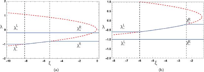
Figure 2. Sketches of Riemann invariants of two types of rarefaction wave structures. (a) ${\lambda }_{+}^{L}={\lambda }_{+}^{R}=-0.2,{\lambda }_{-}^{L}=-1,{\lambda }_{-}^{R}=-0.8$; (b) ${\lambda }_{+}^{L}=-0.6,{\lambda }_{+}^{R}=-0.2,{\lambda }_{-}^{L}={\lambda }_{-}^{R}=-1$. |
3.2. Dispersive shock waves
This study examines the structure of DSWs governed by the Whitham modulation equations (54 ). The evolution of modulated nonlinear periodic waves is characterized through four Riemann invariants r1, r2, r3 and r4 in the Whitham system. Specifically, the DSW profiles emerge when either r2 or r3 varies, while the remaining three invariants remain constant.
In the same way, we introduce the self-similar variable $\xi =\frac{x}{t}$, the Whitham modulation equations (54 ) can be rewritten as 83 ) and (84 ) define the implicit functional relationships of r2 and r3 with respect to ξ. As illustrated in Figure 4, for the parameter ρi, there exist two left intersection points L1 and L2. This configuration generates two corresponding right intersection points R1 and R2, resulting in two distinct paths L1 → R1 and L2 → R2. These paths correspond to equations (51 ) and (52 ), respectively. Substituting equation (51 ) into (33 ) yields the waveforms depicted in figures 3(b) and (c). Similarly, substituting equation (52 ) into (38 ) produces the waveforms shown in figures 3(e) and (f). As illustrated in cases (a) and (b) of figures 3(a) and (d), the edge Whitham velocities for these scenarios are determined by functional combinations of the Riemann invariants:
$\begin{eqnarray}\begin{array}{r}\left({v}_{i}-\xi \right)\frac{{\rm{d}}{r}_{i}}{{\rm{d}}\xi }=0.\end{array}\end{eqnarray}$
Consequently, two distinct types of DSWs can be naturally classified: $\begin{eqnarray}\begin{array}{l}(a)\,{r}_{1}={r}_{+}^{R},\,{r}_{3}={r}_{+}^{L},\,{r}_{4}={r}_{-}^{L}={r}_{-}^{R},\\ {v}_{2}\left({r}_{+}^{R},{r}_{2},{r}_{+}^{L},{r}_{-}^{L}\right)=\xi ,\end{array}\end{eqnarray}$
$\begin{eqnarray}\begin{array}{l}(b)\,{r}_{1}={r}_{+}^{L}={r}_{+}^{R},\,{r}_{2}={r}_{-}^{R},\,{r}_{4}={r}_{-}^{L},\\ {v}_{3}\left({r}_{+}^{L},{r}_{-}^{R},{r}_{3},{r}_{-}^{L}\right)=\xi .\end{array}\end{eqnarray}$
The DSW generated in case (a) is designated as DSW-I, while the DSW arising in case (b) is labeled DSW-II. Figures 3(a) and (d) respectively demonstrate the distributions of the Riemann invariants of DSWs in cases (a) and (b). The final expressions in equations ( $\begin{eqnarray}\begin{array}{rcl}(a)\quad {s}^{L} & = & {v}_{2}\left({r}_{+}^{L},{r}_{+}^{R},{r}_{+}^{R},{r}_{-}^{L}\right)\\ & = & 2{r}_{+}^{L}\left(2{r}_{+}^{R}+{r}_{-}^{L}\right)-\frac{3}{2}{\left({r}_{+}^{L}+2{r}_{+}^{R}+{r}_{-}^{L}\right)}^{2}\\ & & +2\left({r}_{+}^{R}+2{r}_{-}^{L}\right),\end{array}\end{eqnarray}$
$\begin{eqnarray}{s}^{R}={v}_{2}\left({r}_{+}^{L},{r}_{+}^{L},{r}_{+}^{R},{r}_{-}^{R}\right)=\frac{-48{\left({r}_{+}^{L}\right)}^{3}+6{r}_{+}^{L}{\left({r}_{+}^{R}-{r}_{-}^{R}\right)}^{2}+24{\left({r}_{+}^{L}\right)}^{2}\left({r}_{+}^{R}+{r}_{-}^{R}\right)+3{\left({r}_{+}^{R}-{r}_{-}^{R}\right)}^{2}\left({r}_{+}^{R}+{r}_{-}^{R}\right)}{2\left(2{r}_{+}^{L}-{r}_{+}^{R}-{r}_{-}^{R}\right)},\end{eqnarray}$
$\begin{eqnarray}(b)\quad {s}^{L}={v}_{3}\left({r}_{+}^{L},{r}_{-}^{L},{r}_{-}^{R},{r}_{-}^{R}\right)=\frac{-48{\left({r}_{-}^{R}\right)}^{3}+6{r}_{-}^{R}{\left({r}_{+}^{L}-{r}_{-}^{L}\right)}^{2}+24{\left({r}_{-}^{R}\right)}^{2}\left({r}_{+}^{L}+{r}_{-}^{L}\right)+3{\left({r}_{+}^{L}-{r}_{-}^{L}\right)}^{2}\left({r}_{+}^{L}+{r}_{-}^{L}\right)}{2\left(2{r}_{-}^{R}-{r}_{+}^{L}-{r}_{-}^{L}\right)},\end{eqnarray}$
$\begin{eqnarray}\begin{array}{rcl}{s}^{R} & = & {v}_{3}\left({r}_{+}^{L},{r}_{-}^{L},{r}_{-}^{L},{r}_{-}^{R}\right)\\ & = & 2{r}_{+}^{L}\left(2{r}_{-}^{L}+,{r}_{-}^{R}\right)-\frac{3}{2}{\left({r}_{+}^{L}+2{r}_{-}^{L}+,{r}_{-}^{R}\right)}^{2}\\ & & +2\left({r}_{-}^{L}+2{r}_{-}^{R}\right).\end{array}\end{eqnarray}$
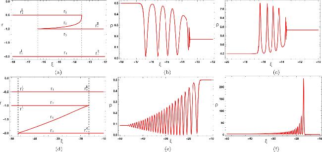
Figure 3. Sketches of Riemann invariants and two possible basic dispersive shock waves structures and their corresponding dispersive shock waves. (a) ${r}_{+}^{L}=-0.5,{r}_{+}^{R}=-1,{r}_{-}^{L}={r}_{-}^{R}=-2$; (d) ${r}_{+}^{L}={r}_{+}^{R}=-0.5,{r}_{-}^{L}=-1,{r}_{-}^{R}=-2$. |
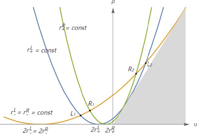
Figure 4. The curves are formed by the relationship between the variables ρ and u, where there are exist two paths from the left boundary to the right boundary. |
3.3. Trigonometric (contact) dispersive shock waves
When the Riemann invariants on both sides of the discontinuity satisfy ${r}_{-}^{L}={r}_{-}^{R}$ and ${r}_{+}^{L}={r}_{+}^{R}$, a novel type of wave structure emerges. This structure is referred to as a contact DSW. Under this condition, the parabolic curves corresponding to the constant Riemann invariants ${r}_{-}^{L}$ and ${r}_{+}^{R}$ coincide with each other, resulting in the disappearance of the conventional cnoidal DSW. Instead, a path connecting the left and right states—which are identical and defined by the intersection points of these two parabolas is formed, as illustrated in Figure 5. It is crucial to emphasize that such a wave can only arise when the left and right boundary points reside on opposite sides of the u = 0 axis, i.e. in different monotonicity regions.
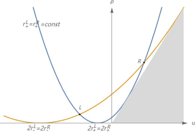
Figure 5. Curves corresponding to constant Riemann invariants and the transition path of a trigonometric dispersive shock wave in the (ρ, u) plane. The boundary points possess identical Riemann invariant values, ${r}_{-}^{L}={r}_{-}^{R}$ and ${r}_{+}^{L}={r}_{+}^{R}$. |
Along the parabolic arc connecting points L and R, the two largest Riemann invariants must satisfy the identity r1 = r2, and at the left edge, they must equal the boundary values ${r}_{1}={r}_{2}={r}_{3}={r}_{+}^{L}={r}_{+}^{R}$. This leads to the schematic diagram of the Riemann invariants shown in Figure 6.
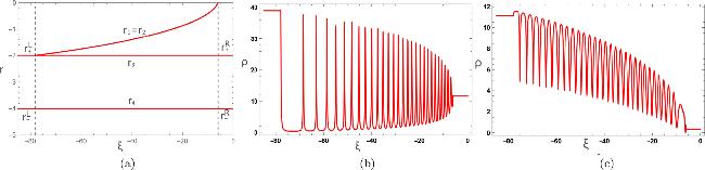
Figure 6. Sketches of Riemann invariants and two possible trigonometric dispersive shock waves structures and their corresponding dispersive shock waves. (a) ${r}_{+}^{L}={r}_{+}^{R}=-2,{r}_{-}^{L}={r}_{-}^{R}=-4$. |
Along this solution path, the elliptic modulus is m = 0, and the solution of the Whitham modulation equation (60 ) is given by: 51 ) into (33 ) yields the waveforms depicted in figures 3(b) and (c). Similarly, substituting equation (52 ) into (38 ) produces the waveforms shown in figures 6(b) and (c). The edge velocities are obtained as:
$\begin{eqnarray}\begin{array}{l}{v}_{1}\,=\,{v}_{2}=\frac{-48{r}_{1}^{3}+6{r}_{1}{\left({r}_{+}^{L}-{r}_{-}^{L}\right)}^{2}+24{r}_{1}^{2}\left({r}_{+}^{L}+{r}_{-}^{L}\right)+3{\left({r}_{+}^{L}-{r}_{-}^{L}\right)}^{2}\left({r}_{+}^{L}+{r}_{-}^{L}\right)}{2\left(2{r}_{1}-{r}_{+}^{L}-{r}_{-}^{L}\right)}=\xi ,\end{array}\end{eqnarray}$
respectively. Substituting equation ( $\begin{eqnarray}\begin{array}{rcl}{s}^{L} & = & {v}_{1}\left({r}_{+}^{L},{r}_{+}^{L},{r}_{+}^{L},{r}_{-}^{L}\right)\\ & = & -\left[\frac{15}{2}{\left({r}_{+}^{L}\right)}^{2}+3{r}_{+}^{L}{r}_{-}^{L}+\frac{3}{2}{\left({r}_{-}^{L}\right)}^{2}\right],\end{array}\end{eqnarray}$
$\begin{eqnarray}\begin{array}{rcll}{s}^{R} & = & {v}_{1}\left(r1,r1,{r}_{+}^{R},{r}_{-}^{R},),\,\right)\,=\, & \frac{-48{r}_{1}^{3}+6{r}_{1}{\left({r}_{+}^{R}-{r}_{-}^{R}\right)}^{2}+24{r}_{1}^{2}\left({r}_{+}^{R}+{r}_{-}^{R}\right)+3{\left({r}_{+}^{R}-{r}_{-}^{R}\right)}^{2}\left({r}_{+}^{R}+{r}_{-}^{R}\right)}{2\left(2{r}_{1}-{r}_{+}^{R}-{r}_{-}^{R}\right)}.\end{array}\end{eqnarray}$
3.4. Combined shocks
When the boundary points reside in different monotonicity regions, an elementary wave structure connecting two plateau states emerges, known as combined shocks. This structure is characterized by one Riemann invariant remaining constant (${r}_{-}^{L}={r}_{-}^{R}$), while the boundary values of the other invariant differ. Specifically, as illustrated in Figure 7(a), the case ${r}_{+}^{L}\lt {r}_{+}^{R}$ is observed, whereas Figure 7(b) demonstrates the scenario with ${r}_{+}^{L}\gt {r}_{+}^{R}$. The corresponding schematic diagrams of the Riemann invariants are presented in Figure 8.
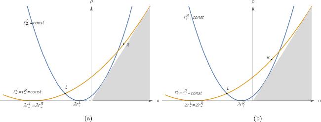
Figure 7. Curves corresponding to constant Riemann invariants and the transition path of combined shocks in the (ρ, u) plane, (a) represents the rarewaves with r+ = const combined with the cnoidal shock; (b) represents the trigonometric shock with r− = const combined with the cnoidal shock. |
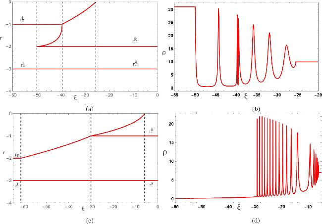
Figure 8. Sketches of Riemann invariants and two possible combined shocks structures and their corresponding combined shocks. (a) ${r}_{+}^{L}=-1,{r}_{+}^{R}=-2,{r}_{-}^{L}={r}_{-}^{R}=-3$; (c) ${r}_{+}^{L}=-2,{r}_{+}^{R}=-1,{r}_{-}^{L}={r}_{-}^{R}=-3$. |
As shown in Figure 8(a), the oscillatory region located between the two plateaus consists of two subregions: one containing four distinct Riemann invariants corresponding to a DSW, and the other satisfying r1 = r2, corresponding to a trigonometric DSW, with no plateau existing between them. Consequently, this results in a combined wave structure formed by the superposition of a DSW and a trigonometric DSW, as illustrated in Figure 8(b). The edge velocities can be expressed as:
$\begin{eqnarray}\begin{array}{rcl}{S}_{A} & = & {v}_{2}\left({r}_{+}^{L},{r}_{+}^{R},{r}_{+}^{R},{r}_{-}^{R}\right)\\ & = & 2{r}_{+}^{L}\left(2{r}_{+}^{R}+{r}_{-}^{R}\right)-\frac{3}{2}{\left({r}_{+}^{L}+2{r}_{+}^{R}+{r}_{-}^{R}\right)}^{2}\\ & & +2\left({r}_{+}^{R}+2{r}_{-}^{R}\right),\end{array}\end{eqnarray}$
$\begin{eqnarray}\begin{array}{l}{S}_{B}\,=\,{v}_{2}\left({r}_{+}^{L},{r}_{+}^{L},{r}_{+}^{R},{r}_{-}^{R}\right)=\frac{-48{\left({r}_{+}^{L}\right)}^{3}+6{r}_{+}^{L}{\left({r}_{+}^{R}-{r}_{-}^{R}\right)}^{2}+24{\left({r}_{+}^{L}\right)}^{2}\left({r}_{+}^{R}+{r}_{-}^{R}\right)+3{\left({r}_{+}^{R}-{r}_{-}^{R}\right)}^{2}\left({r}_{+}^{R}+{r}_{-}^{R}\right)}{2\left(2{r}_{+}^{L}-{r}_{+}^{R}-{r}_{-}^{R}\right)},\end{array}\end{eqnarray}$
$\begin{eqnarray}\begin{array}{r}{S}_{C}={v}_{1}\left(0,0,{r}_{+}^{R},{r}_{-}^{R}\right)=-\frac{3{\left({r}_{+}^{R}-{r}_{-}^{R}\right)}^{2}}{2}.\end{array}\end{eqnarray}$
As shown in Figure 8(c), we obtain a single trigonometric DSW region connected to a rarefaction wave. As illustrated in Figure 8(b), the edge velocities are given by: $\begin{eqnarray}{S}_{A}={v}_{+}\left({r}_{+}^{L},{r}_{-}^{R}\right)=-\left[\frac{15}{2}{\left({r}_{+}^{L}\right)}^{2}+3{r}_{+}^{L}{r}_{-}^{R}+\frac{3}{2}{\left({r}_{-}^{R}\right)}^{2}\right],\end{eqnarray}$
$\begin{eqnarray}{S}_{B}={v}_{+}\left({r}_{+}^{R},{r}_{-}^{R}\right)=-\left[\frac{15}{2}{\left({r}_{+}^{R}\right)}^{2}+3{r}_{+}^{R}{r}_{-}^{R}+\frac{3}{2}{\left({r}_{-}^{R}\right)}^{2}\right],\end{eqnarray}$
$\begin{eqnarray}{S}_{C}={v}_{1}\left(0,0,{r}_{+}^{L},{r}_{-}^{R}\right)=-\frac{3{\left({r}_{+}^{L}-{r}_{-}^{R}\right)}^{2}}{2}.\end{eqnarray}$
4. Complete classification of the solution to Riemann problem
Under the discontinuous initial conditions defined by equation (1 ), the interplay of ${r}_{+}=\frac{1}{2}\left(u-\rho +\sqrt{\rho \left(\rho -2u\right)}\right)$ and ${r}_{-}=\frac{1}{2}\left(u-\rho -\sqrt{\rho \left(\rho -2u\right)}\right)$ generates two parabolic profiles
$\begin{eqnarray}\begin{array}{r}\rho =-\frac{{\left(u-2{r}_{+}\right)}^{2}}{4{r}_{+}},\quad \rho =-\frac{{\left(u-2{r}_{-}\right)}^{2}}{4{r}_{-}},\end{array}\end{eqnarray}$
with $2{r}_{+}^{L}\gt 2{r}_{-}^{L}$. The classification framework initiates from two boundary points situated on one side of the axis u = 0, which partitions the (ρ, u) plane into two distinct monotonicity regions. We focus on configurations where the boundary points reside within the left monotonic region (u < 0). As depicted in Figure 9, the (ρ, u) plane is divided into six regions by two parabolic trajectories defined by the aforementioned parabolic constraints. Within each region, the hierarchical ordering of the Riemann invariants ${r}_{+}^{L},{r}_{-}^{L},{r}_{+}^{R}$ and ${r}_{-}^{R}$ can be readily determined through systematic analysis. It is seen that there are six regions in the (ρ, u) plane, which are marked as A, B, C, D, E, F and satisfy the following order relations: $\begin{eqnarray}\begin{array}{l}A:{r}_{-}^{L}\lt {r}_{+}^{L}\lt {r}_{-}^{R}\lt {r}_{+}^{R},\quad B:{r}_{-}^{L}\lt {r}_{-}^{R}\lt {r}_{+}^{L}\lt {r}_{+}^{R},\\ C:{r}_{-}^{L}\lt {r}_{-}^{R}\lt {r}_{+}^{R}\lt {r}_{+}^{L},\quad D:{r}_{-}^{R}\lt {r}_{-}^{L}\lt {r}_{+}^{L}\lt {r}_{+}^{R},\\ E:{r}_{-}^{R}\lt {r}_{-}^{L}\lt {r}_{+}^{R}\lt {r}_{+}^{L},\quad F:{r}_{-}^{R}\lt {r}_{+}^{R}\lt {r}_{-}^{L}\lt {r}_{+}^{L}.\end{array}\end{eqnarray}$
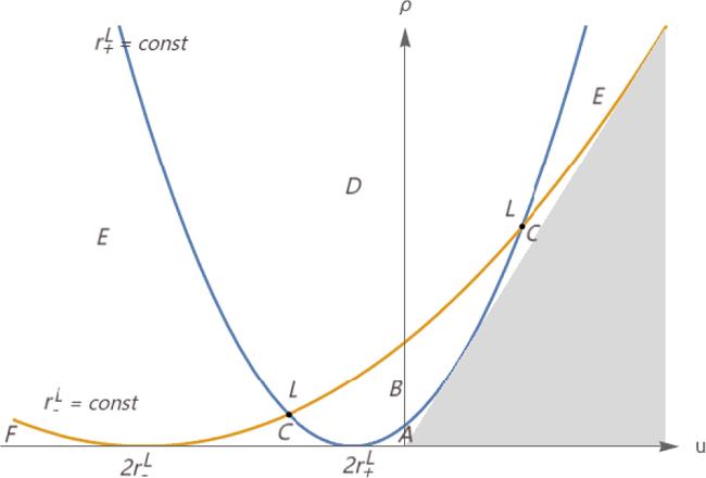
Figure 9. Regions in the (ρ, u) plane corresponding to different classes of the solution for Riemann problem. |
In the following, a complete classification of solutions to the Riemann problem for equation (1 ) is established by analyzing the six characteristic zones and their corresponding six possible wave structures. The distribution of Riemann invariants and the self-similar solutions to the Riemann problem (64 ) are analyzed one case by one case, and it is gratifying that all the theoretical results agree well with the direct numerical simulations.
Case A. ${r}_{-}^{L}\lt {r}_{+}^{L}\lt {r}_{-}^{R}\lt {r}_{+}^{R}$
In this case, only two types of rarefaction waves emerge with no presence of DSWs. As illustrated in figures 10(a) and (b), the domain is partitioned into five regions from left to right: plateau, RW-I, vacuum region, RW-II, and another plateau. The Whitham velocities at the left and right edges of each region are expressed respectively as follows:
$\begin{eqnarray}\begin{array}{rcl}{S}_{A} & = & {v}_{-}\left({r}_{+}^{L},{r}_{-}^{L}\right)\\ & = & -\left(\frac{3}{2}{\left({r}_{+}^{L}\right)}^{2}+3{r}_{+}^{L}{r}_{-}^{L}+\frac{15}{2}{\left({r}_{-}^{L}\right)}^{2}\right),\end{array}\end{eqnarray}$
$\begin{eqnarray}\begin{array}{r}{S}_{B}={v}_{+}\left({r}_{+}^{L},{r}_{+}^{L}\right)=-12{\left({r}_{+}^{L}\right)}^{2},\end{array}\end{eqnarray}$
$\begin{eqnarray}\begin{array}{r}{S}_{C}={v}_{-}\left({r}_{-}^{R},{r}_{-}^{R}\right)=-12{\left({r}_{-}^{R}\right)}^{2},\end{array}\end{eqnarray}$
$\begin{eqnarray}\begin{array}{rcl}{S}_{D} & = & {v}_{+}\left({r}_{+}^{R},{r}_{-}^{R}\right)\\ & = & -\left(\frac{15}{2}{\left({r}_{+}^{R}\right)}^{2}+3{r}_{+}^{R}{r}_{-}^{R}+\frac{3}{2}{\left({r}_{-}^{R}\right)}^{2}\right).\end{array}\end{eqnarray}$
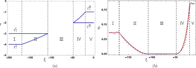
Figure 10. The distribution of Riemann invariants and the corresponding wave structures in Case A. (a) ${r}_{+}^{L}=-3$, ${r}_{+}^{R}=-1$, ${r}_{-}^{L}=-4$, ${r}_{-}^{R}=-2$; (b) displays the wave patterns of the density function ρ derived from Whitham theory at t = 1. The solid red line represents the results from the Whitham modulation theory, and the blue dashed line represents the results from the numerical simulation. |
Case B. ${r}_{-}^{L}\lt {r}_{-}^{R}\lt {r}_{+}^{L}\lt {r}_{+}^{R}$
This case shares similarities with Case A in the absence of DSWs, with only two types of rarefaction waves. However, distinct from Case A, no vacuum region emerges here, instead, the wave structure comprises alternating plateaux. As shown in figures 11(a) and (b), the five regions from left to right are: plateau, RW-I, plateau, RW-II, and plateau. The boundary velocities between adjacent intervals are expressed left-to-right as follows:
$\begin{eqnarray}\begin{array}{rcl}{S}_{A} & = & {v}_{-}\left({r}_{+}^{L},{r}_{-}^{L}\right)\\ & = & -\left[\frac{3}{2}{\left({r}_{+}^{L}\right)}^{2}+3{r}_{+}^{L}{r}_{-}^{L}+\frac{15}{2}{\left({r}_{-}^{L}\right)}^{2}\right],\end{array}\end{eqnarray}$
$\begin{eqnarray}\begin{array}{rcl}{S}_{B} & = & {v}_{-}\left({r}_{+}^{L},{r}_{-}^{R}\right)\\ & = & -\left[\frac{3}{2}{\left({r}_{+}^{L}\right)}^{2}+3{r}_{+}^{L}{r}_{-}^{R}+\frac{15}{2}{\left({r}_{-}^{R}\right)}^{2}\right],\end{array}\end{eqnarray}$
$\begin{eqnarray}\begin{array}{rcl}{S}_{C} & = & {v}_{+}\left({r}_{+}^{L},{r}_{-}^{R}\right)\\ & = & -\left[\frac{15}{2}{\left({r}_{+}^{L}\right)}^{2}+3{r}_{+}^{L}{r}_{-}^{R}+\frac{3}{2}{\left({r}_{-}^{R}\right)}^{2}\right],\end{array}\end{eqnarray}$
$\begin{eqnarray}\begin{array}{rcl}{S}_{D} & = & {v}_{+}\left({r}_{+}^{R},{r}_{-}^{R}\right)\\ & = & -\left[\frac{15}{2}{\left({r}_{+}^{R}\right)}^{2}+3{r}_{+}^{R}{r}_{-}^{R}+\frac{3}{2}{\left({r}_{-}^{R}\right)}^{2}\right].\end{array}\end{eqnarray}$
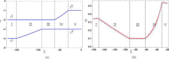
Figure 11. The distribution of Riemann invariants and the corresponding wave structures in Case B: (a) ${r}_{+}^{L}=-2$, ${r}_{+}^{R}=-1$, ${r}_{-}^{L}=-4$, ${r}_{-}^{R}=-3$; (b) displays the wave patterns of the density function ρ derived from Whitham theory at t = 1. The solid red line represents the results from the Whitham modulation theory, and the blue dashed line represents the results from the numerical simulation. |
Case C. ${r}_{-}^{L}\lt {r}_{-}^{R}\lt {r}_{+}^{R}\lt {r}_{+}^{L}$
In this case, the wave structure features a combination of one rarefaction wave and one DSW. As depicted in figures 12(a) and (b), the domain is divided into five regions from left to right: plateau, RW-I, plateau, DSW-I and plateau. The left and right edge Whitham velocities for each region are expressed in left-to-right order as follows:
$\begin{eqnarray}\begin{array}{rcl}{S}_{A} & = & {v}_{-}\left({r}_{+}^{L},{r}_{-}^{L}\right)\\ & = & -\left[\frac{3}{2}{\left({r}_{+}^{L}\right)}^{2}+3{r}_{+}^{L}{r}_{-}^{L}+\frac{15}{2}{\left({r}_{-}^{L}\right)}^{2}\right],\end{array}\end{eqnarray}$
$\begin{eqnarray}\begin{array}{rcl}{S}_{B} & = & {v}_{-}\left({r}_{+}^{L},{r}_{-}^{R}\right)\\ & = & -\left[\frac{3}{2}{\left({r}_{+}^{L}\right)}^{2}+3{r}_{+}^{L}{r}_{-}^{R}+\frac{15}{2}{\left({r}_{-}^{R}\right)}^{2}\right],\end{array}\end{eqnarray}$
$\begin{eqnarray}\begin{array}{rcll}{S}_{C} & = & {v}_{2}\left({r}_{+}^{L},{r}_{+}^{R},{r}_{+}^{R},{r}_{-}^{R}\right)\,= & 2{r}_{+}^{L}\left(2{r}_{+}^{R}+{r}_{-}^{R}\right)-\frac{3}{2}{\left({r}_{+}^{L}+2{r}_{+}^{R}+{r}_{-}^{R}\right)}^{2}+2\left({r}_{+}^{R}+2{r}_{-}^{R}\right),\end{array}\end{eqnarray}$
$\begin{eqnarray}\begin{array}{r}\begin{array}{l}{S}_{D}={v}_{2}\left({r}_{+}^{L},{r}_{+}^{L},{r}_{+}^{R},{r}_{-}^{R}\right)=\frac{-48{\left({r}_{+}^{L}\right)}^{3}+6{r}_{+}^{L}{\left({r}_{+}^{R}-{r}_{-}^{R}\right)}^{2}+24{\left({r}_{+}^{L}\right)}^{2}\left({r}_{+}^{R}+{r}_{-}^{R}\right)+3{\left({r}_{+}^{R}-{r}_{-}^{R}\right)}^{2}\left({r}_{+}^{R}+{r}_{-}^{R}\right)}{2\left(2{r}_{+}^{L}-{r}_{+}^{R}-{r}_{-}^{R}\right)}.\end{array}\end{array}\end{eqnarray}$
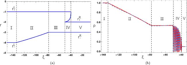
Figure 12. The distribution of Riemann invariants and the corresponding wave structures in Case C: (a) ${r}_{+}^{L}=-1$, ${r}_{+}^{R}=-2$, ${r}_{-}^{L}=-4$, ${r}_{-}^{R}=-3$; (b) displays the wave patterns of the density function ρ derived from Whitham theory at t = 5. The solid red line represents the results from the Whitham modulation theory, and the blue dashed line represents the results from the numerical simulation. |
Case D. ${r}_{-}^{R}\lt {r}_{-}^{L}\lt {r}_{+}^{L}\lt {r}_{+}^{R}$
This case, similar to Case C, features a rarefaction wave and a DSW. However, distinct from Case C, the wave types differ: as illustrated in figures 13(a) and (b), the spatial domain is partitioned into five regions from left to right: plateau, DSW-II, plateau, DRW-I, and plateau. The left and right edge Whitham velocities for each region are sequentially defined from left to right as follows:
$\begin{eqnarray}\begin{array}{r}\begin{array}{l}\,{S}_{A}={v}_{3}\left({r}_{+}^{L},{r}_{-}^{L},{r}_{-}^{R},{r}_{-}^{R}\right)\,=\frac{-48{\left({r}_{-}^{R}\right)}^{3}+6{r}_{-}^{R}{\left({r}_{+}^{L}-{r}_{-}^{L}\right)}^{2}+24{\left({r}_{-}^{R}\right)}^{2}\left({r}_{+}^{L}+{r}_{-}^{L}\right)+3{\left({r}_{+}^{L}-{r}_{-}^{L}\right)}^{2}\left({r}_{+}^{L}+{r}_{-}^{L}\right)}{2\left(2{r}_{-}^{R}-{r}_{+}^{L}-{r}_{-}^{L}\right)},\end{array}\end{array}\end{eqnarray}$
$\begin{eqnarray}\begin{array}{rcll}{S}_{B} & = & {v}_{3}\left({r}_{+}^{L},{r}_{-}^{L},{r}_{-}^{L},{r}_{-}^{R}\right)\,= & 2{r}_{+}^{L}\left(2{r}_{-}^{L}+{r}_{-}^{R}\right)-\frac{3}{2}{\left({r}_{+}^{L}+2{r}_{-}^{L}+{r}_{-}^{R}\right)}^{2}+2\left({r}_{-}^{L}+2{r}_{-}^{R}\right),\end{array}\end{eqnarray}$
$\begin{eqnarray}\begin{array}{rcl}{S}_{C} & = & {v}_{+}\left({r}_{+}^{L},{r}_{-}^{R}\right)=-\left[\frac{15}{2}{\left({r}_{+}^{L}\right)}^{2}+3{r}_{+}^{L}{r}_{-}^{R}+\frac{3}{2}{\left({r}_{-}^{R}\right)}^{2}\right],\end{array}\end{eqnarray}$
$\begin{eqnarray}\begin{array}{rcl}{S}_{D} & = & {v}_{+}\left({r}_{+}^{R},{r}_{-}^{R}\right)=-\left[\frac{15}{2}{\left({r}_{+}^{R}\right)}^{2}+3{r}_{+}^{R}{r}_{-}^{R}+\frac{3}{2}{\left({r}_{-}^{R}\right)}^{2}\right].\end{array}\end{eqnarray}$
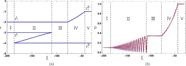
Figure 13. The distribution of Riemann invariants and the corresponding wave structures in Case D: (a) ${r}_{+}^{L}=-2$, ${r}_{+}^{R}=-1$, ${r}_{-}^{L}=-3$, ${r}_{-}^{R}=-4$; (b) displays the wave patterns of the density function ρ derived from Whitham theory at t = 1. The solid red line represents the results from the Whitham modulation theory, and the blue dashed line represents the results from the numerical simulation. |
Case E. ${r}_{-}^{R}\lt {r}_{-}^{L}\lt {r}_{+}^{R}\lt {r}_{+}^{L}$
In this case, two DSWs emerge with no presence of rarefaction waves. As shown in figures 14(a) and (b), the spatial domain is partitioned into five regions from left to right: plateau, DSW-II, plateau, DSW-I, and plateau. The left and right edge Whitham velocities for each region are sequentially defined in left-to-right order as follows:
$\begin{eqnarray}\begin{array}{r}\begin{array}{l}{S}_{A}={v}_{3}\left({r}_{+}^{L},{r}_{-}^{L},{r}_{-}^{R},{r}_{-}^{R}\right)=\frac{-48{\left({r}_{-}^{R}\right)}^{3}+6{r}_{-}^{R}{\left({r}_{+}^{L}-{r}_{-}^{L}\right)}^{2}+24{\left({r}_{-}^{R}\right)}^{2}\left({r}_{+}^{L}+{r}_{-}^{L}\right)+3{\left({r}_{+}^{L}-{r}_{-}^{L}\right)}^{2}\left({r}_{+}^{L}+{r}_{-}^{L}\right)}{2\left(2{r}_{-}^{R}-{r}_{+}^{L}-{r}_{-}^{L}\right)},\end{array}\end{array}\end{eqnarray}$
$\begin{eqnarray}\begin{array}{rcll}{S}_{B} & = & {v}_{3}\left({r}_{+}^{L},{r}_{-}^{L},{r}_{-}^{L},{r}_{-}^{R}\right)\,= & 2{r}_{+}^{L}\left(2{r}_{-}^{L}+{r}_{-}^{R}\right)-\frac{3}{2}{\left({r}_{+}^{L}+2{r}_{-}^{L}+{r}_{-}^{R}\right)}^{2}+2\left({r}_{-}^{L}+2{r}_{-}^{R}\right),\end{array}\end{eqnarray}$
$\begin{eqnarray}\begin{array}{rcll}{S}_{C} & = & {v}_{2}\left({r}_{+}^{L},{r}_{+}^{R},{r}_{+}^{R},{r}_{-}^{R}\right)\,= & 2{r}_{+}^{L}\left(2{r}_{+}^{R}+{r}_{-}^{R}\right)-\frac{3}{2}{\left({r}_{+}^{L}+2{r}_{+}^{R}+{r}_{-}^{R}\right)}^{2}+2\left({r}_{+}^{R}+2{r}_{-}^{R}\right),\end{array}\end{eqnarray}$
$\begin{eqnarray}\begin{array}{r}\begin{array}{l}{S}_{D}={v}_{2}\left({r}_{+}^{L},{r}_{+}^{L},{r}_{+}^{R},{r}_{-}^{R}\right)=\frac{-48{\left({r}_{+}^{L}\right)}^{3}+6{r}_{+}^{L}{\left({r}_{+}^{R}-{r}_{-}^{R}\right)}^{2}+24{\left({r}_{+}^{L}\right)}^{2}\left({r}_{+}^{R}+{r}_{-}^{R}\right)+3{\left({r}_{+}^{R}-{r}_{-}^{R}\right)}^{2}\left({r}_{+}^{R}+{r}_{-}^{R}\right)}{2\left(2{r}_{+}^{L}-{r}_{+}^{R}-{r}_{-}^{R}\right)}.\end{array}\end{array}\end{eqnarray}$
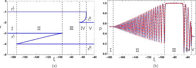
Figure 14. The distribution of Riemann invariants and the corresponding wave structures in Case E: (a) ${r}_{+}^{L}=-2$, ${r}_{+}^{R}=-1$, ${r}_{-}^{L}=-3$, ${r}_{-}^{R}=-4$; (b) displays the wave patterns of the density function ρ derived from Whitham theory at t = 1. The solid red line represents the results from the Whitham modulation theory, and the blue dashed line represents the results from the numerical simulation. |
Case F. ${r}_{-}^{R}\lt {r}_{+}^{R}\lt {r}_{-}^{L}\lt {r}_{+}^{L}$
In this case, three DSWs emerge in the absence of rarefaction waves, one of which is non-modulated DSW. As illustrated in figures 15(a) and (b), the spatial domain is partitioned into five regions from left to right: plateau, DSW-II, non-modulated DSW, DSW-I, and plateau. The left and right edge Whitham velocities for each interval are sequentially defined in left-to-right order as follows:
$\begin{eqnarray}\begin{array}{r}\begin{array}{l}{S}_{A}={v}_{3}\left({r}_{+}^{L},{r}_{-}^{L},{r}_{-}^{R},{r}_{-}^{R}\right)=\frac{-48{\left({r}_{-}^{R}\right)}^{3}+6{r}_{-}^{R}{\left({r}_{+}^{L}-{r}_{-}^{L}\right)}^{2}+24{\left({r}_{-}^{R}\right)}^{2}\left({r}_{+}^{L}+{r}_{-}^{L}\right)+3{\left({r}_{+}^{L}-{r}_{-}^{L}\right)}^{2}\left({r}_{+}^{L}+{r}_{-}^{L}\right)}{2\left(2{r}_{-}^{R}-{r}_{+}^{L}-{r}_{-}^{L}\right)},\end{array}\end{array}\end{eqnarray}$
$\begin{eqnarray}\begin{array}{r}{S}_{B}={v}_{3}\left({r}_{+}^{L},{r}_{-}^{L},{r}_{+}^{R},{r}_{-}^{R}\right),\end{array}\end{eqnarray}$
$\begin{eqnarray}\begin{array}{r}{S}_{C}={v}_{2}\left({r}_{+}^{L},{r}_{-}^{L},{r}_{+}^{R},{r}_{-}^{R}\right),\end{array}\end{eqnarray}$
$\begin{eqnarray}\begin{array}{r}\begin{array}{l}{S}_{D}={v}_{2}\left({r}_{+}^{L},{r}_{+}^{L},{r}_{+}^{R},{r}_{-}^{R}\right)\,=\frac{-48{\left({r}_{+}^{L}\right)}^{3}+6{r}_{+}^{L}{\left({r}_{+}^{R}-{r}_{-}^{R}\right)}^{2}+24{\left({r}_{+}^{L}\right)}^{2}\left({r}_{+}^{R}+{r}_{-}^{R}\right)+3{\left({r}_{+}^{R}-{r}_{-}^{R}\right)}^{2}\left({r}_{+}^{R}+{r}_{-}^{R}\right)}{2\left(2{r}_{+}^{L}-{r}_{+}^{R}-{r}_{-}^{R}\right)}.\end{array}\end{array}\end{eqnarray}$
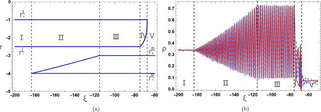


Figure 15. The distribution of Riemann invariants and the corresponding wave structures in Case F. ${r}_{+}^{L}=-1$, ${r}_{+}^{R}=-3$, ${r}_{-}^{L}=-2.5$ and ${r}_{-}^{R}=-4$; (b) displays the wave patterns of the density function ρ derived from Whitham theory at t = 1. The solid red line represents the results from the Whitham modulation theory, and the blue dashed line represents the results from the numerical simulation. |
5. Conclusions
In summary, this work has delivered a complete classification of the Riemann problem for the third-order focusing KN equation, extending beyond the established framework for its second-order counterpart. The principal innovation lies in revealing how third-order dispersion and quintic nonlinearity fundamentally reshape the wave dynamics, yielding distinctive features absent in the classical theory. Specifically, the characteristic velocities and Riemann invariants derived here exhibit essentially different mathematical structures from those of the standard KN model, leading to unique waveform configurations—such as the stable vacuum region observed in Case A. These phenomena, together with the six complete solution regimes identified, underscore that higher-order terms do not merely perturb existing solutions but qualitatively enrich the landscape of dispersive hydrodynamic states. Our findings thus establish a foundational reference for future studies on more complex integrable systems within the KN hierarchy.
Finally, from our obtained results in the present paper, we realize that there are some differences between the dynamical behaviors of the focusing and defocusing cases. The difference in the values of the Riemann invariants leads to distinct waveforms for rarefaction waves and DSWs in the focusing and defocusing equations. Moreover, for the focusing equation, we present a type of combined shock wave. This complex waveform structure deeply reveals the unique dynamical behaviors arising from the interaction between the high-order dispersion term and the quintic nonlinear term, enriching our understanding of dispersive hydrodynamics in integrable systems. Furthermore, we present the first fully classified solution to the Riemann problem for the focusing equation, detailing six fundamental wave structures. Crucially, each case is supported by direct numerical simulations that show excellent agreement with the predictions of Whitham modulation theory.