

1. Introduction
The inflationary framework has emerged as a compelling extension of standard Big Bang cosmology, resolving several of its fundamental shortcomings, including the flatness, horizon, and monopole problems. Moreover, it provides a natural mechanism for generating the primordial fluctuations that seed the formation of large-scale structures in the Universe [1–4]. These primordial inhomogeneities arise from quantum fluctuations of the inflaton field that were stretched to cosmological scales during the inflationary expansion, eventually manifesting as temperature anisotropies in the cosmic microwave background (CMB). Their statistical properties are typically characterized by two principal observables: the scalar spectral index ns, which describes the scale dependence of scalar perturbations, and the tensor-to-scalar ratio r, which measures the relative strength of tensor modes compared to the scalar modes.
Recent measurements by the Atacama Cosmology Telescope (ACT) have led to updated constraints on these parameters. Compared to earlier Planck data [5], ACT-based results tend to favor slightly higher values of ns. For instance, a joint analysis using both Planck and ACT datasets (P-ACT) yields ns = 0.9709 ± 0.0038 [6, 7], while further inclusion of CMB lensing and BAO data from DESI (denoted P-ACT-LB) shifts the preferred value to ns = 0.9743 ± 0.0034 [8, 9]. This upward shift, approximately 1σ from the Planck-only estimate, has important implications for inflationary model building.
Many well-studied models, including hilltop-type scenarios [10], α-attractors [11, 12], Starobinsky’s R2 inflation [1], and Higgs inflation with strong nonminimal couplings [13, 14], predict a universal attractor behavior for the spectral index of the form ns ≈ 1−2/N, where N denotes the number of e-folds before the end of inflation. With N = 60, this gives ns ≈ 0.9667, which agrees well with the Planck best-fit value, but falls just outside the 1σ region favored by the P-ACT-LB results. This mild tension motivates a re-examination of existing models and prompts the exploration of new mechanisms capable of naturally generating a slightly higher scalar spectral index while remaining consistent with other observational constraints.
Several strategies have been proposed to address this issue. These include revisiting models with strong nonminimal couplings [15, 16], incorporating detailed reheating dynamics into inflationary predictions [17–22], and exploring broader theoretical frameworks such as multi-field inflation, warm inflation, or modifications of general relativity [23–38]. In this work, we explore the viability of constant-roll tachyon inflation as a mechanism compatible with current CMB observations. Unlike conventional slow-roll inflation driven by a canonical scalar field evolving slowly along a flat potential, tachyon inflation arises naturally in the context of string theory. In particular, the decay of unstable D-branes is described by a rolling tachyon condensate governed by a nonstandard Dirac–Born–Infeld (DBI)-type effective action [39–43]. This framework has been extensively studied for its cosmological applications and is known to produce a nearly scale-invariant power spectrum [44–46]. Besides the slow-roll condition, the inflation model with a constant-roll condition [47–60], where one of the slow-roll parameters remains constant, has attracted attention for its richer dynamics and potential observational signatures, such as distinctive non-Gaussian features [61–63], the production of primordial black holes [64–89], and the generation of scalar-induced gravitational waves [90–113].
Finally, tachyon inflation provides a string-motivated realization of non-canonical single-field inflation, distinct from canonical slow-roll or α-attractor models in its kinetic structure and predictions. The constant-roll extension further enriches the dynamics by introducing a controllable deviation from the slow-roll attractor, enhancing the model’s flexibility to accommodate high-precision CMB data such as those from ACT while retaining theoretical consistency. For a broader classification of inflationary scenarios in extended gravity frameworks, see [114]. In this work, we investigate whether tachyon inflation under a constant-roll condition can accommodate the scalar spectral index values favored by recent P-ACT-LB observations, while simultaneously producing a tensor-to-scalar ratio consistent with current limits.
The rest of the paper is organized as follows. In section 2 , we briefly introduce the predictions of tachyon inflation models. In section 3 , we implement the constant-roll condition and analyze the resulting dynamics, identifying parameter regimes consistent with observational constraints. Section 5 concludes with a summary and discussion.
2. The tachyon inflation
In scenarios involving more general scalar fields, the kinetic term does not necessarily follow the conventional canonical form. A notable example arises in string theory, where the tachyon condensate is effectively modeled by a scalar field possessing a noncanonical kinetic structure. Such a configuration is capable of driving inflation independently of the potential. The dynamics of the rolling tachyon are governed by an effective action of the form 6 ) and (7 ), the first two horizon-flow slow-roll parameters can be expressed in terms of the potential as follows [46]:
$\begin{eqnarray}{S}_{T}=-\int {{\rm{d}}}^{4}x\sqrt{-g}\,V(T)\sqrt{1+{g}^{\mu \nu }{\partial }_{\mu }T{\partial }_{\nu }T},\end{eqnarray}$
where T is the tachyon field, V(T) is the potential, and we choose the units ${M}_{{\rm{p}}{\rm{l}}}=1/\sqrt{8\pi G}=c=1$. In the homogeneous and isotropic universe, the background evolution is governed by the Friedmann equation and the equation of motion for the tachyon field, $\begin{eqnarray}{H}^{2}=\frac{1}{3}\frac{V}{\sqrt{1-{\dot{T}}^{2}}},\end{eqnarray}$
$\begin{eqnarray}\frac{\ddot{T}}{1-{\dot{T}}^{2}}+3H\dot{T}+\frac{{V}_{,T}}{V}=0,\end{eqnarray}$
where $H=\dot{a}/a$ is the Hubble parameter, a dot denotes the derivative with respect to the cosmic time, and V,T = dV/dT. In the slow-roll regime, the slow-roll conditions are $\begin{eqnarray}{\dot{T}}^{2}\ll 1,\end{eqnarray}$
$\begin{eqnarray}\quad \ddot{T}\ll 3H\dot{T}.\end{eqnarray}$
Under these slow-roll conditions, the background equations during inflation become $\begin{eqnarray}{H}^{2}\approx \frac{V}{3},\end{eqnarray}$
$\begin{eqnarray}3H\dot{T}\approx -{V}_{,T}/V.\end{eqnarray}$
The e-folding number of the inflation before the end of inflation is given by $\begin{eqnarray}N(t)={\int }_{t}^{{t}_{{\rm{e}}}}H(t){\rm{d}}t,\end{eqnarray}$
where the subscript ‘e’ indicates the value at the end of inflation. In terms of the number of e-folds N, we can introduce the horizon-flow slow-roll parameters [115] $\begin{eqnarray}{\epsilon }_{0}=\frac{{H}_{* }}{H},\end{eqnarray}$
$\begin{eqnarray}{\epsilon }_{i+1}=-\frac{{\rm{d}}\mathrm{ln}| {\epsilon }_{i}| }{{\rm{d}}N},\end{eqnarray}$
where the subscript ‘*’ denotes the moment of horizon crossing, and H* is the Hubble parameter at horizon crossing for a specific reference scale. By applying the slow-roll background equations ( $\begin{eqnarray}{\epsilon }_{1}=-\frac{\dot{H}}{{H}^{2}}\approx {\epsilon }_{V},\end{eqnarray}$
$\begin{eqnarray}{\epsilon }_{2}=2\frac{\ddot{T}}{H\dot{T}}\approx -{\eta }_{V}+6{\epsilon }_{V},\end{eqnarray}$
where the potential slow-roll parameters are defined as $\begin{eqnarray}{\epsilon }_{V}=\frac{1}{2}\frac{{V}_{,T}^{2}}{{V}^{3}},\quad {\eta }_{V}=\frac{2{V}_{,TT}}{{V}^{2}}.\end{eqnarray}$
By using the slow-roll parameters and the slow-roll background equations, the e-folding number becomes $\begin{eqnarray}N(T)\approx {\int }_{{T}_{{\rm{e}}}}^{T}\frac{{V}^{2}}{{V}_{,T}}{\rm{d}}T.\end{eqnarray}$
2.1. Perturbations
For scalar perturbations, the evolution of the Fourier modes is governed by the Mukhanov–Sasaki equation [46], 15 ) in the slow-roll approximation yields the power spectrum of scalar perturbations [46],
$\begin{eqnarray}{v}_{k}^{{\prime\prime} }+\left({c}_{{\rm{s}}}^{2}{k}^{2}-\frac{{z}^{{\prime\prime} }}{z}\right){v}_{k}=0,\end{eqnarray}$
where a prime denotes the derivative with respect to the conformal time dτ = dt/a, ${c}_{{\rm{s}}}^{2}=1-{\dot{T}}^{2}$ is the effective sound speed, and $\begin{eqnarray}z=\frac{\sqrt{3}a\dot{T}}{\sqrt{1-{\dot{T}}^{2}}}.\end{eqnarray}$
In terms of the slow-roll parameters, the quantity z″/z can be approximated as [46] $\begin{eqnarray}\frac{{z}^{{\prime\prime} }}{z}\approx {a}^{2}{H}^{2}\left(2-{\epsilon }_{1}+\frac{3}{2}{\epsilon }_{2}\right)=\frac{{\nu }^{2}-1/4}{{\tau }^{2}},\end{eqnarray}$
where the parameter ν is $\begin{eqnarray}\nu =\frac{3}{2}+{\epsilon }_{1}+\frac{1}{2}{\epsilon }_{2}.\end{eqnarray}$
Solving equation ( $\begin{eqnarray}{P}_{\zeta }=\frac{{k}^{3}}{2{\pi }^{2}}{\left|\frac{{v}_{k}}{z}\right|}^{2}\approx {\left.\frac{{H}^{2}}{8{\pi }^{2}{\epsilon }_{1}}\right|}_{{c}_{{\rm{s}}}k=aH}.\end{eqnarray}$
The scalar spectral index is then given by [44, 46] $\begin{eqnarray}{n}_{{\rm{s}}}-1={\left.\frac{{\rm{d}}\mathrm{ln}{P}_{\zeta }}{{\rm{d}}\mathrm{ln}k}\right|}_{{c}_{{\rm{s}}}k=aH}=-2{\epsilon }_{1}-{\epsilon }_{2}.\end{eqnarray}$
A similar procedure yields the power spectrum for tensor perturbations [46]19 ) and (21 ), the tensor-to-scalar ratio is given by [44, 46]Appendix .
$\begin{eqnarray}{P}_{{\rm{T}}}\approx {\left.\frac{2{H}^{2}}{{\pi }^{2}}\right|}_{k=aH}.\end{eqnarray}$
Combining equations ( $\begin{eqnarray}r\approx 16{\epsilon }_{1}.\end{eqnarray}$
For more detailed derivations of the background and perturbation equations in tachyon inflation, please see 2.2. The reconstruction
Combining equations (8 ) and (11 ), we find that the first slow-roll parameter can be expressed as 23 ) and (24 ) into the expression for the scalar spectral index equation (20 ) yields
$\begin{eqnarray}{\epsilon }_{1}=\frac{3}{2}{\dot{T}}^{2}\approx \frac{{V}_{,N}}{2V},\end{eqnarray}$
and the second slow-roll parameter becomes $\begin{eqnarray}{\epsilon }_{2}=-\frac{{\rm{d}}\mathrm{ln}{\epsilon }_{1}}{{\rm{d}}N}.\end{eqnarray}$
Substituting equations ( $\begin{eqnarray}{n}_{{\rm{s}}}-1=-2{\epsilon }_{1}+\frac{{\rm{d}}{\rm{ln}}{\epsilon }_{1}}{{\rm{d}}N}={\left({\rm{ln}}\frac{{V}_{,N}}{{V}^{2}}\right)}_{,N}.\end{eqnarray}$
These relations show that specifying any single observable quantity, such as the scalar spectral index ns, the tensor-to-scalar ratio r or the slow-roll parameter, as a function of the number of e-folds N, is sufficient to determine the full inflationary dynamics. In particular, once a specific parametrization like ε1(N) or ns(N) is chosen, all other background quantities, including the Hubble parameter H(N), the potential V(N), and the evolution of the inflaton field, can be derived systematically.
To reconstruct the inflationary potential in terms of the field variable, we can proceed as follows. First, using the chain rule and the background equations, the relation between the field T and the number of e-folds can be approximately expressed as
$\begin{eqnarray}{\rm{d}}T\approx \pm \frac{\sqrt{{V}_{,N}}}{V}\,{\rm{d}}N,\end{eqnarray}$
where V,N = dV/dN, and the sign is determined by the direction of the field evolution, i.e. it matches the sign of dV/dT.In this paper, we adopt the positive sign, ‘+’. Integrating this equation gives the functional T(N), which can then be inverted to obtain N(T), and hence reconstruct the potential V(T) from the known V(N).3. Constant-roll inflation with constant ηV
Traditional inflationary models generally require the potential function to satisfy the slow-roll conditions. Under these conditions, the predictions of the inflationary model can more easily align with observational results. However, not all inflationary models are of the slow-roll type. For instance, there is the ultra-slow-roll inflation model [61], which features an inflection point in the potential function. This type of model can be used to enhance the primordial curvature power spectrum, thereby promoting the formation of primordial black holes [116, 117]. When neither the slow-roll nor the ultra-slow-roll conditions are met, the situation tends to become more complicated. To simplify the analysis, it is common to assume that one of the slow-roll parameters remains constant while the other slow-roll parameters still satisfy the slow-roll conditions [62]. In this section, we investigate constant-roll inflation under the assumption that the potential slow-roll parameter ηV remains constant. For comparison, different constant-roll conditions in tachyon inflation, analyzed against Planck 2015 data [118], were studied in [57]. We remark that our analysis is performed at the effective field theory level and does not attempt to provide a fundamental resolution of the eta-problem [119, 120]. In the tachyon framework, the non-canonical kinetic structure can soften the impact of a large ηV, but a complete theoretical treatment of the eta-problem would require embedding in a UV-complete model, which lies beyond the scope of this work.
Combining equations (23 ) and (24 ), we obtain the relation 11 ). From the definition of ηV, it follows that the inflationary potential V(T) satisfies a second-order differential equation, which leads to a solution expressible in terms of the Weierstrass function. To proceed analytically, we impose the boundary condition εV(N = 0) = 1, corresponding to the end of inflation. Solving equation (27 ) under this condition yields 28 ) into equation (25 ) for the scalar spectral index, we obtain [54]
$\begin{eqnarray}{\eta }_{V}\approx \frac{{\rm{d}}\mathrm{ln}{\epsilon }_{V}}{{\rm{d}}N}+6{\epsilon }_{V}.\end{eqnarray}$
Note that εV ≈ ε1 as given in equation ( $\begin{eqnarray}{\epsilon }_{V}=-\frac{{\eta }_{V}}{(6-{\eta }_{V}){{\rm{e}}}^{-{\eta }_{V}N}-6}.\end{eqnarray}$
The corresponding tensor-to-scalar ratio is then given by [54] $\begin{eqnarray}r=-\frac{16{\eta }_{V}}{(6-{\eta }_{V}){{\rm{e}}}^{-{\eta }_{V}N}-6}.\end{eqnarray}$
Substituting equation ( $\begin{eqnarray}{n}_{{\rm{s}}}-1=\frac{8{\eta }_{V}}{(6-{\eta }_{V}){{\rm{e}}}^{-{\eta }_{V}N}-6}+{\eta }_{V}.\end{eqnarray}$
In contrast to traditional slow-roll inflation models, which typically start from a specific inflationary potential to compute observable quantities, constant-roll inflation begins with a constant-roll condition to derive observables and then reconstructs the corresponding potential function. Once a value of ηV is chosen and a specific e-folding number (e.g. N = 60 in this paper) is fixed, we can compute the scalar spectral index and tensor-to-scalar ratio predicted by the constant-roll inflation model using equations (29 ) and (30 ). By scanning over different values of ηV, we obtain a range of values for the scalar spectral index and tensor-to-scalar ratio. Comparing these predictions with observational data allows us to assess whether constant-roll inflation can explain the latest observations and, simultaneously, to determine the observational constraints on ηV.
The comparison between the theoretical predictions for the scalar spectral index in equation (30 ) and the tensor-to-scalar ratio in equation (29 ) and current observational constraints is shown in Figure 1. The constraints labeled as ‘P-ACT-LB-BK18’ in Figure 1 are derived from the combination of Planck, ACT, and CMB lensing + BAO data (denoted P-ACT-LB), together with the B-mode polarization measurements from the BICEP/Keck Array 2018 (BK18) observations at the South Pole [121], for which the resulting contours are shown in figure 10 of the ACT DR6 analysis [7]. The region inside the contours corresponds to the observationally allowed values of the scalar spectral index ns and the tensor-to-scalar ratio r, with the inner and outer contours indicating the 1σ and 2σ confidence regions, respectively. The black solid line labeled as N = 60 shows the predictions of the constant-roll inflation model, with each point corresponding to a specific value of ηV (increasing from left to right as indicated by the arrow). We find that tachyon inflation with a constant potential slow-roll ηV parameter is consistent with the most recent data. To lie within the 1σ confidence region of the P-ACT-LB-BK18 data, the constant-roll parameter must satisfy −0.016 < ηV < −0.0096; for consistency with the 2σ region, the allowed range is extended to −0.025 < ηV < 0.00063. Consequently, within the permitted parameter range where ∣ηV∣ ≪ 1 holds, the constant-roll scenario effectively reduces to the slow-roll regime. The predictions of the ns and r from different ηV is displayed in table 1.
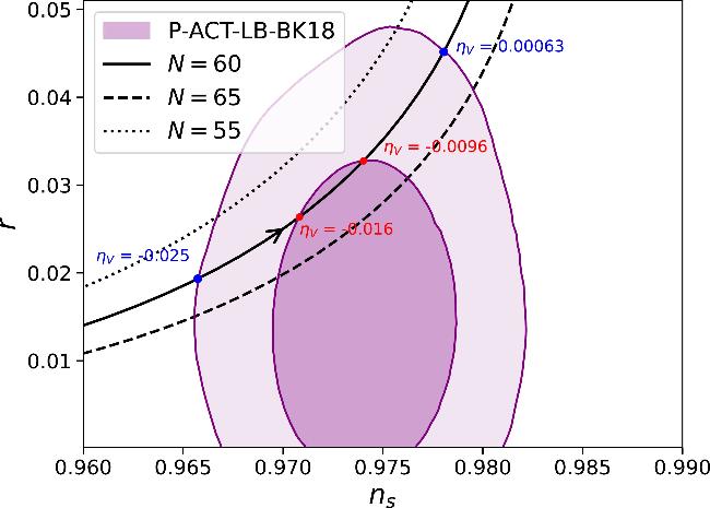
Figure 1. The figure contrasts theoretical results with observational constraints, with the purple contours showing the 1σ and 2σ confidence regions obtained from the P-ACT-LB-BK18 dataset. The black solid curve shows the predictions from equations ( |
Table 1. The predictions of ns and r for different ηV with N = 60. |
| ηV | −0.025 | −0.015 | −0.01 | −0.005 | −0.0001 | 0.0001 | 0.0005 |
| ns | 0.9655 | 0.9714 | 0.9738 | 0.9760 | 0.9778 | 0.9779 | 0.9793 |
| r | 0.019 | 0.027 | 0.032 | 0.038 | 0.044 | 0.045 | 0.051 |
By substituting equation (28 ) into equation (23 ), we obtain the potential of the constant-roll tachyon inflation as a function of the number of e-folds N26 ), the relation between the tachyon field T and the number of e-folds N can be written as 31 ) and (34 ). For illustration, we consider the case with ηV = −0.012 and N* = 60, which yields the observational predictions ns = 0.9729, r = 0.030. Using these parameter values, the reconstructed potential for constant-roll tachyon inflation is shown in Figure 2, and displayed by the black line.
$\begin{eqnarray}V(N)={V}_{0}{\left|6{{\rm{e}}}^{{\eta }_{V}N}-6+{\eta }_{V}\right|}^{\frac{1}{3}}.\end{eqnarray}$
The overall amplitude V0 is given by $\begin{eqnarray}\begin{array}{rcl}{V}_{0} & = & \frac{3{\pi }^{2}{A}_{{\rm{s}}}{r}_{* }}{2}\\ & & \times {\left|\frac{8-8{n}_{{\rm{s}}* }-{r}_{* }}{\left[8-8{n}_{{\rm{s}}* }-4{r}_{* }\right]\left[7-{n}_{{\rm{s}}* }-{r}_{* }/2\right]}\right|}^{1/3},\end{array}\end{eqnarray}$
where the amplitude of the scalar power spectrum is $\mathrm{ln}(1{0}^{10}{A}_{{\rm{s}}})=3.044$ [5], ns* = ns(N*), r* = r(N*), and N* = 60. From equation ( $\begin{eqnarray}{\rm{d}}T=\frac{2}{{\eta }_{V}}\sqrt{\frac{2| {\eta }_{V}| }{{V}_{0}}}\,\frac{1}{{(6{x}^{2}-6+{\eta }_{V})}^{2/3}}{\rm{d}}x,\end{eqnarray}$
where $x={{\rm{e}}}^{{\eta }_{V}N/2}$. This equation can be integrated in terms of the hypergeometric function 2F1, yielding $\begin{eqnarray}T-{T}_{0}={T}_{f}(N)-{T}_{f}(0),\end{eqnarray}$
with $\begin{eqnarray}\begin{array}{rcl}{T}_{f}(N) & = & \frac{2}{{\eta }_{V}}\sqrt{\frac{2| {\eta }_{V}| }{{V}_{0}}}\frac{\exp ({\eta }_{V}N/2)}{{(6-{\eta }_{V})}^{2/3}}\\ & & {\times \,}_{2}{F}_{1}\left(\frac{1}{2},\frac{2}{3};\frac{3}{2};\frac{6{{\rm{e}}}^{{\eta }_{V}N}}{6-{\eta }_{V}}\right)n({\eta }_{V}),\end{array}\end{eqnarray}$
where T0 is an integration constant, and n(ηV) = 1 for ηV < 0, and n(ηV) = e2πi/3 for ηV > 0. The final form of the potential V(T) as a function of the tachyon field T can be obtained by combining equations (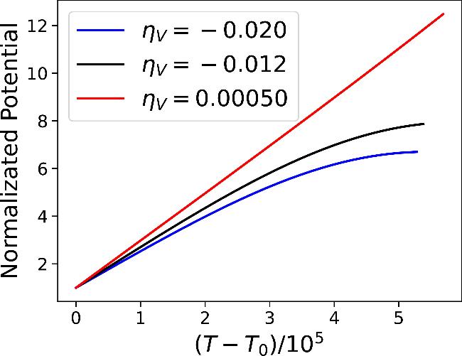


Figure 2. The potential, normalized at T − T0 = 0, for constant-roll tachyon inflation. The black curve corresponds to ηV = −0.012 (with predictions ns = 0.9729, r = 0.030), while the blue and red curves represent ηV = −0.020 and ηV = 0.000 50, respectively, both lying within the 2σ region. The observational data favor concave potentials associated with negative values of ηV. |
To further explore the sensitivity of the potential to the choice of ηV, Figure 2 presents two additional representative cases: ηV = −0.020 (within the 2σ region, indicated by the blue curve) and ηV = 0.000 50 (a small positive value allowed within 2σ, shown by the red curve). The resulting potentials show significant differences: negative ηV produces concave shapes, whereas positive ηV results in convex forms. The ACT constraints disfavor convex potentials, which aligns with the behavior in canonical slow-roll inflation, where recent data also suggest a preference for concave potentials [7].
In the present model, both convex and concave potential shapes correspond to smooth monotonic profiles, which do not produce the small-scale enhancement of scalar perturbations required for PBH formation or significant SIGW. Such amplification typically occurs only near inflection points or during transient non-attractor phases.
4. Discussion
It should be emphasized that the choice of N = 60 adopted in our analysis implicitly corresponds to the assumption of instantaneous reheating. When reheating lasts for a finite period and is characterized by a non-trivial effective equation of state, the inflationary e-folding number is no longer fixed but can change significantly. Introducing this additional degree of freedom leads to shifted predictions for (ns, r), which in turn relaxes the constraints on ηV. From this perspective, the parameter space of tachyon constant-roll inflation may be even more easily reconciled with the current ACT constraints once realistic reheating scenarios are taken into account. Under the hypothesis that the reheating phase is characterized by a fixed equation of state w${}_{{\rm{re}}}$ and that radiation domination commences immediately once reheating ends, the connection between the number of e-folds N during inflationary and the e-folds N${}_{{\rm{re}}}$ during reheating can be written as [54, 122]31 ). The reheating e-folding number depends logarithmically on Ve and εV; therefore, in an approximate analysis, these quantities can be treated as constants. In addition, the reheating temperature mainly depends on the reheating e-folding number and the equation of state w${}_{{\rm{re}}}$. Therefore, we have the approximate relation
$\begin{eqnarray}{N}_{{\rm{r}}{\rm{e}}}=\frac{4}{1-3{w}_{{\rm{r}}{\rm{e}}}}\left(56.94-N-\frac{1}{4}\mathrm{ln}{V}_{{\rm{e}}}+\frac{1}{2}\mathrm{ln}{\epsilon }_{V}(N)\right),\end{eqnarray}$
$\begin{eqnarray}{T}_{{\rm{r}}{\rm{e}}}=\exp \left[-\frac{3{N}_{{\rm{r}}{\rm{e}}}(1+{w}_{{\rm{r}}{\rm{e}}})}{4}\right]{\left[\frac{3\sqrt{3}{V}_{{\rm{e}}}}{10.675{\pi }^{2}}\right]}^{1/4},\end{eqnarray}$
where Ve = V(N = 0) is given by equation ( $\begin{eqnarray}N\approx 60-\frac{(1-3{w}_{{\rm{r}}{\rm{e}}}){N}_{{\rm{r}}{\rm{e}}}}{4},\end{eqnarray}$
$\begin{eqnarray}{T}_{{\rm{r}}{\rm{e}}}\approx 0.005\exp \left[-\frac{3{N}_{{\rm{r}}{\rm{e}}}(1+{w}_{{\rm{r}}{\rm{e}}})}{4}\right].\end{eqnarray}$
For instantaneous reheating (Nre = 0), the e-folding number during inflation is N = 60. A stiffer equation of state (wre > 1/3) increases the e-folding number during inflation N, whereas a softer one (wre < 1/3) decreases it. A larger e-folding number N leads to better agreement with observational data, as illustrated in Figure 1, where the black dashed curve denotes the case with N = 65 and the black dotted curve denotes the case N = 55. Consequently, reheating with wre > 1/3 relaxes the constraint on ηV, while wre < 1/3 tightens it. As long as N${}_{{\rm{re}}}$ is not too large, the temperature at the end of reheating stays above the Big Bang nucleosynthesis bound.Another implication of the allowed parameter space concerns primordial non-Gaussianities. Tachyon inflation, as a DBI-type model with non-canonical kinetic terms, can in principle produce enhanced higher-order correlations [123]. For example, for a reduced sound speed cs < 1, equilateral-type non-Gaussianity amplitude is approximately ${f}_{NL}^{\,\rm{equil}\,}\approx ({c}_{{\rm{s}}}^{-2}-1)/3$ [124], which can be significant when cs ≪ 1. However, in the constant-roll regime considered here, the values of ηV consistent with the ACT constraints correspond to small slow-roll parameters and a sound speed close to unity. In this sense, the constant-roll scenario effectively satisfies the slow-roll condition, and the resulting level of non-Gaussianity is expected to be suppressed with the order of ${f}_{NL}^{\,\rm{equil}\,}\sim { \mathcal O }({\epsilon }_{1},{\eta }_{V},{c}_{{\rm{s}}}-1)\sim 1{0}^{-2}$ [123, 124], and safely within the current CMB bounds ${f}_{NL}^{\,\rm{equil}\,}=-26\pm 47$ [125]. This confirms that, in the observationally allowed region, the constant-roll tachyon scenario remains compatible with the observed Gaussianity of primordial perturbations.
At the level of current CMB constraints, tachyon constant-roll inflation and other constant-roll scenarios, such as f(R) or α-attractors, yield nearly degenerate predictions for ns and r, making them observationally indistinguishable with present data. The key distinction lies in their theoretical structure: the tachyon model originates from a DBI-type action and allows for a reduced sound speed cs < 1, which can, in principle, imprint distinctive signatures in higher-order statistics, although it is expected to be small in the parameter range considered here. Future measurements of non-Gaussianity and related observables may, therefore, provide a promising avenue to break this degeneracy.
Finally, we briefly comment on the UV sensitivity of the reconstructed potential. Since the parameter region relevant to ACT constraints satisfies ∣ηV∣ ≪ 1, quantum corrections and higher-order DBI terms remain perturbative and do not affect the concave shape qualitatively. This ensures the stability of the inflationary dynamics at the effective field theory level, while possible UV completions may be addressed in string-theoretic embeddings of tachyon inflation.
5. Conclusion
Recent observations reported by the ACT show a discrepancy with the predictions of a broad class of standard inflationary scenarios. In this work, we explored tachyon inflation under a constant-roll condition, where the slow-roll parameter ηV = 2V,TT/V2 is taken to be constant. We demonstrated that this framework can yield predictions consistent with the P-ACT-LB-BK18 data. Specifically, to be consistent with the 1σ confidence region, the constant-roll parameter must satisfy −0.016 < ηV <−0.0096, while agreement with the 2σ region requires −0.025 < ηV < 0.000 63. These results suggest that constant-roll tachyon inflation offers a viable alternative to slow-roll models in light of current observational constraints.
Finally, we note that tachyon models, due to their non-canonical kinetic structure, are generally expected to generate a certain level of primordial non-Gaussianity. In the constant-roll scenario studied here, however, the absolute value of ηV remains small and the dynamics effectively fall within the slow-roll regime, so the predicted non-Gaussianity is suppressed and well within the current observational limits.
Appendix Formulation of tachyon inflation
A.1. The background
The tachyon condensate is governed by a DBI-type action,
$\begin{eqnarray}{S}_{{\rm{T}}}=-\int {{\rm{d}}}^{4}x\sqrt{-g}\,V(T)\sqrt{1+{g}^{\mu \nu }{\partial }_{\mu }T{\partial }_{\nu }T},\end{eqnarray}$
where we work in reduced Planck units ${M}_{{\rm{p}}{\rm{l}}}=1/\sqrt{8\pi G}\,=c=1$. For a systematic treatment, we employ the ADM decomposition [126], $\begin{eqnarray}{\rm{d}}{s}^{2}=-{{\mathscr{N}}}^{2}{\rm{d}}{t}^{2}+{h}_{ij}\left({\rm{d}}{x}^{i}+{N}^{i}{\rm{d}}t\right)\left({\rm{d}}{x}^{j}+{N}^{j}{\rm{d}}t\right),\end{eqnarray}$
where ${\mathscr{N}}$ is the lapse, Ni the shift, and hij the spatial metric. The combined gravitational and tachyonic action becomes $\begin{eqnarray}\begin{array}{rcl}S & = & \displaystyle \int {{\rm{d}}}^{4}x{\mathscr{N}}\sqrt{h}\left\{\frac{1}{2}\left[{\,}^{(3)}R+\frac{1}{{{\mathscr{N}}}^{2}}({E}^{ij}{E}_{ij}-{E}^{2})\right]\right.\\ & & -\left.V{\left(1-\frac{{\dot{T}}^{2}}{{{\mathscr{N}}}^{2}}\right)}^{\frac{1}{2}}\right\},\end{array}\end{eqnarray}$
with $\begin{eqnarray}{E}_{ij}=\frac{1}{2}\left({\dot{h}}_{ij}-{{\rm{\nabla }}}_{i}{N}_{j}-{{\rm{\nabla }}}_{j}{N}_{i}\right),\quad E={h}^{ij}{E}_{ij}.\end{eqnarray}$
Since ${\mathscr{N}}$ and Ni have no kinetic terms, their variation yields the constraint equations: $\begin{eqnarray}{{\rm{\nabla }}}_{i}\left[\frac{1}{{\mathscr{N}}}({E}_{j}^{i}-{h}_{ij}E)\right]=0,\end{eqnarray}$
$\begin{eqnarray}{}^{(3)}R-\frac{1}{{{\mathscr{N}}}^{2}}({E}^{ij}{E}_{ij}-{E}^{2})-2V{\left(1-\frac{{\dot{T}}^{2}}{{{\mathscr{N}}}^{2}}\right)}^{-\frac{1}{2}}=0.\end{eqnarray}$
Specializing to a spatially flat FRW background with ${\mathscr{N}}=1,\ {N}^{i}=0,\ {h}_{ij}={a}^{2}{\delta }_{ij}$, the Hamiltonian constraint reduces to the Friedmann equation,
$\begin{eqnarray}{H}^{2}=\frac{1}{3}\frac{V}{\sqrt{1-{\dot{T}}^{2}}}.\end{eqnarray}$
The tachyon behaves as an effective fluid with $\begin{eqnarray}\rho =\frac{V}{\sqrt{1-{\dot{T}}^{2}}},\end{eqnarray}$
$\begin{eqnarray}w=\frac{p}{\rho }={\dot{T}}^{2}-1.\end{eqnarray}$
The equation of motion for the tachyon field is $\begin{eqnarray}\frac{\ddot{T}}{1-{\dot{T}}^{2}}+3H\dot{T}+\frac{{V}_{,T}}{V}=0,\end{eqnarray}$
where V,T = dV/dT. Together with the Friedmann equation, we get $\begin{eqnarray}\dot{H}=-\frac{3}{2}{H}^{2}{\dot{T}}^{2}.\end{eqnarray}$
From equation (A11 ), the acceleration of the scale factor reads A17 ) and (A20 ), we get
$\begin{eqnarray}\frac{\ddot{a}}{a}=\dot{H}+{H}^{2}={H}^{2}\left(1-\frac{3}{2}{\dot{T}}^{2}\right),\end{eqnarray}$
so inflation requires ${\dot{T}}^{2}\lt 2/3$. In the slow-roll regime, $\begin{eqnarray}{\dot{T}}^{2}\ll 1,\end{eqnarray}$
$\begin{eqnarray}\quad \ddot{T}\ll 3H\dot{T},\end{eqnarray}$
the background equations reduce to $\begin{eqnarray}{H}^{2}\approx \frac{V}{3},\end{eqnarray}$
$\begin{eqnarray}3H\dot{T}\approx -{V}_{,T}/V.\end{eqnarray}$
The number of e-folds $N(t)=\mathrm{ln}({a}_{{\rm{e}}}/a)$ before the end of inflation is $\begin{eqnarray}N(t)={\int }_{t}^{{t}_{{\rm{e}}}}H(t){\rm{d}}t.\end{eqnarray}$
Introducing the horizon-flow parameters [115], $\begin{eqnarray}{\epsilon }_{0}=\frac{{H}_{* }}{H},\end{eqnarray}$
$\begin{eqnarray}{\epsilon }_{i+1}=-\frac{{\rm{d}}\mathrm{ln}| {\epsilon }_{i}| }{{\rm{d}}N},\end{eqnarray}$
one obtains, for tachyon inflation [46], $\begin{eqnarray}{\epsilon }_{1}=-\frac{\dot{H}}{{H}^{2}}=\frac{3}{2}{\dot{T}}^{2}\approx \frac{1}{2}\frac{{V}_{,T}^{2}}{{V}^{3}},\end{eqnarray}$
$\begin{eqnarray}{\epsilon }_{2}=2\frac{\ddot{T}}{H\dot{T}}\approx -2\frac{{V}_{,TT}}{{V}^{2}}+3\frac{{V}_{,T}^{2}}{{V}^{3}}.\end{eqnarray}$
From equations ( $\begin{eqnarray}N(T)=\pm \sqrt{\frac{3}{2}}\,{\int }_{T}^{{T}_{{\rm{e}}}}\frac{H}{\sqrt{{\epsilon }_{1}}}{\rm{d}}T\approx {\int }_{{T}_{{\rm{e}}}}^{T}\frac{{V}^{2}}{{V}_{,T}}{\rm{d}}T,\end{eqnarray}$
where the ± sign is the same as the sign of $\dot{T}$.A.2. The perturbations
In the spatially flat gauge, the perturbations can be written in the form A5 ) and the Hamiltonian constraint (A6 ), and expanding consistently to linear order, one finds that the transverse part of the shift vector vanishes, ${N}_{i}^{{\rm{T}}}=0$ and
$\begin{eqnarray}\begin{array}{rcl}\delta T(x,t) & = & 0,\,{\mathscr{N}}=1+{N}_{1},\,{N}_{i}={\partial }_{i}\psi +{N}_{i}^{{\rm{T}}},\\ {h}_{ij} & = & {a}^{2}\left((1+2\zeta +2{\zeta }^{2}){\delta }_{ij}+{\gamma }_{ij}+\displaystyle \frac{1}{2}{\gamma }_{il}{\gamma }_{lj}\right),\end{array}\end{eqnarray}$
where ${\partial }^{i}{N}_{i}^{{\rm{T}}}=0$. Here ζ represents the scalar curvature perturbation, while γij corresponds to tensor fluctuations. The tensor modes are transverse and traceless, i.e. ∂iγij = 0 and hijγij = 0. All variables ${N}_{1},\psi ,{N}_{i}^{{\rm{T}}},\zeta ,$ and γij are treated as first-order quantities. Plugging the above ansatz into the momentum constraint ( $\begin{eqnarray}\begin{array}{rcl}{N}_{1} & = & \frac{\dot{\zeta }}{H},\\ \psi & = & -\frac{\zeta }{{a}^{2}H}+\chi ,\\ {{\rm{\nabla }}}^{2}\chi & = & \frac{3}{2}\frac{{\dot{T}}^{2}}{1-{\dot{T}}^{2}}\dot{\zeta }.\end{array}\end{eqnarray}$
After eliminating constraints, the quadratic action for ζ reads $\begin{eqnarray}S=-\frac{3}{2}\int {{\rm{d}}}^{4}x\left[a{\dot{T}}^{2}{({\partial }_{i}\zeta )}^{2}-{a}^{3}\frac{{\dot{T}}^{2}}{1-{\dot{T}}^{2}}{\dot{\zeta }}^{2}\right].\end{eqnarray}$
Defining the canonical variable v = zζ with $\begin{eqnarray}z=\frac{\sqrt{3}a\dot{T}}{\sqrt{1-{\dot{T}}^{2}}},\end{eqnarray}$
and switching to conformal time τ = ∫dt/a, one obtains the Mukhanov–Sasaki form $\begin{eqnarray}S=\int {{\rm{d}}}^{3}x{\rm{d}}\tau \frac{1}{2}\left[{v{}^{{\prime} }}^{2}-{c}_{{\rm{s}}}^{2}{({\partial }_{i}v)}^{2}+\frac{{z}^{{\prime\prime} }}{z}{v}^{2}\right],\end{eqnarray}$
where the sound speed is ${c}_{{\rm{s}}}^{2}=1-{\dot{T}}^{2}$ [44]. In the slow-roll approximation, the effective mass term for the curvature perturbation can be written as [46] $\begin{eqnarray}\frac{{z}^{{\prime\prime} }}{z}\approx {a}^{2}{H}^{2}\left(2-{\epsilon }_{1}+\frac{3}{2}{\epsilon }_{2}\right).\end{eqnarray}$
To quantize the fluctuations, we expand the canonical variable v in Fourier space, $\begin{eqnarray}\hat{v}(\tau ,\overrightarrow{x})=\int \frac{{{\rm{d}}}^{3}k}{{(2\pi )}^{3}}\left[{v}_{k}(\tau ){\hat{a}}_{k}{{\rm{e}}}^{{\rm{i}}\overrightarrow{k}\cdot \overrightarrow{x}}+{v}_{k}^{* }(\tau ){\hat{a}}_{k}^{\dagger }{{\rm{e}}}^{-{\rm{i}}\overrightarrow{k}\cdot \overrightarrow{x}}\right],\end{eqnarray}$
where ${\hat{a}}_{k}$ and ${\hat{a}}_{k}^{\dagger }$ denote annihilation and creation operators. They satisfy the canonical commutation relations, $\begin{eqnarray}\begin{array}{rcl}\left[{\hat{a}}_{k},\,{\hat{a}}_{{k}^{{\prime} }}^{\dagger }\right] & = & {(2\pi )}^{3}{\delta }^{3}(\overrightarrow{k}-\overrightarrow{{k}^{{\prime} }}),\\ \left[{\hat{a}}_{k},\,{\hat{a}}_{{k}^{{\prime} }}\right] & = & \left[{\hat{a}}_{k}^{\dagger },\,{\hat{a}}_{{k}^{{\prime} }}^{\dagger }\right]=0.\end{array}\end{eqnarray}$
The mode functions are normalized through the Wronskian condition, $\begin{eqnarray}{v}_{k}^{{\prime} }{v}_{k}^{* }-{v}_{k}{{v}_{k}^{* }}^{{\prime} }=-{\rm{i}}.\end{eqnarray}$
The vacuum state is chosen as the Bunch–Davies vacuum, defined by ${\hat{a}}_{k}| 0\rangle =0$.From the quadratic action (A27 ) for the perturbations and the background relation (A28 ) above, one obtains the Mukhanov–Sasaki equation for the mode function vk [46]:
$\begin{eqnarray}{v}_{k}^{{\prime\prime} }+\left({c}_{{\rm{s}}}^{2}{k}^{2}-\frac{{\nu }^{2}-1/4}{{\tau }^{2}}\right){v}_{k}=0,\end{eqnarray}$
with the index $\begin{eqnarray}\nu =\frac{3}{2}+{\epsilon }_{1}+\frac{1}{2}{\epsilon }_{2}.\end{eqnarray}$
Imposing the Bunch–Davies initial state and solving the above equation, the curvature perturbation on superhorizon scales approaches a nearly constant value,
$\begin{eqnarray}| {\zeta }_{k}| =\frac{| {v}_{k}| }{z}={2}^{\nu -\frac{5}{2}}\frac{{\rm{\Gamma }}(\nu )}{{\rm{\Gamma }}(3/2)}\frac{H{(1-{\epsilon }_{1})}^{\nu -1/2}}{{c}_{{\rm{s}}}^{1/2}{k}^{3/2}{\epsilon }_{1}^{1/2}}{\left(\frac{{c}_{{\rm{s}}}k}{aH}\right)}^{\frac{3}{2}-\nu }.\end{eqnarray}$
Accordingly, the scalar power spectrum reads [46] $\begin{eqnarray}{P}_{\zeta }=\frac{{k}^{3}}{2{\pi }^{2}}| {\zeta }_{k}{| }^{2}=\left[1-\left(\frac{5}{3}+2C\right){\epsilon }_{1}-C{\epsilon }_{2}\right]{\left.\frac{{H}^{2}}{8{\pi }^{2}{\epsilon }_{1}}\right|}_{{c}_{{\rm{s}}}k=aH},\end{eqnarray}$
where the constant $C=\gamma +\mathrm{ln}2-2\simeq -0.72$. The amplitude and tilt are then $\begin{eqnarray}{A}_{{\rm{s}}}={\left.\frac{{H}^{2}}{8{\pi }^{2}{\epsilon }_{1}}\right|}_{{c}_{{\rm{s}}}k=aH}.\end{eqnarray}$
The scalar spectral tilt is [44, 46] $\begin{eqnarray}{n}_{{\rm{s}}}-1={\left.\frac{{\rm{d}}{\rm{ln}}{P}_{\zeta }}{{\rm{d}}{\rm{ln}}k}\right|}_{{c}_{{\rm{s}}}k=aH}=-2{\epsilon }_{1}-{\epsilon }_{2}.\end{eqnarray}$
Expanding the action (A3 ) to quadratic order in tensor fluctuations γij gives
$\begin{eqnarray}S=\frac{1}{8}\int {{\rm{d}}}^{4}x\left[{a}^{3}{({\dot{\gamma }}_{ij})}^{2}-a{({\gamma }_{ij,k})}^{2}\right].\end{eqnarray}$
The corresponding tensor spectrum is [46] $\begin{eqnarray}{P}_{{\rm{T}}}=[1-2(1+C){\epsilon }_{1}]{\left.\frac{2{H}^{2}}{{\pi }^{2}}\right|}_{k=aH},\end{eqnarray}$
and tensor spectral tilt is [46] $\begin{eqnarray}{n}_{{\rm{T}}}=-2{\epsilon }_{1}[1+{\epsilon }_{1}+(1+C){\epsilon }_{2}].\end{eqnarray}$
Finally, the tensor-to-scalar ratio is obtained as [44, 46] $\begin{eqnarray}r=16{\epsilon }_{1}\left[1-\frac{1}{3}{\epsilon }_{1}+C{\epsilon }_{2}\right].\end{eqnarray}$