

1. Introduction
It has been a century since scientists first attempted to reconcile general relativity with quantum theory [1, 2]. Nonetheless, in the absence of empirical data, a conclusive theoretical model has yet to emerge. The prevailing perspective holds that we cannot obtain such data from laboratory experiments because the test of quantum gravity (QG) needs a Milky Way-sized particle accelerator to touch the Planck length [3]. However, during the inflationary epoch, the tensor perturbations [primordial gravitational waves (GWs)] originate from quantum fluctuations of the gravitational field were amplified and resulted in a characteristic B-modes polarization signal in the cosmic microwave background (CMB) [4]. This signal allows the direct detection of the inflationary epoch and potentially the quantum properties of gravity [4–6]. At present, a multitude of campaigns dedicated to the observation of the CMB B-mode polarization are actively underway (BICEP [7], CLASS [8], Simons Array [9], Simons Observatory [10], etc). In the near future, there will be more observational campaigns with higher precision trying to detect and measure the B-mode polarization in the CMB (AliCPT [11], CMB-S4 [12], etc).
After detecting CMB B-mode polarization, can we say that gravity possesses quantum properties? In fact, GWs can be sourced by any energetically-relevant components during inflation, and particles abundantly produced in the inflationary era would inevitably imprint signatures in primordial B-modes [6]. Furthermore, various post-inflationary processes can generate GWs. For example, a scale-invariant spectrum of gravitational radiation similar to that from inflation can arise from a continuous symmetry-breaking phase transition [13]. GWs can also be produced during the preheating or reheating phases due to explosive particle production, as well as from bubble collisions [14] or the loops arising throughout the cosmological evolution of the cosmic string network [15], which produce a stochastic GW background. These GWs can also affect the CMB B-mode polarization.
Accurately identifying the sources of CMB B-mode polarization is crucial for detecting QG and determining the energy scale of inflation. In order to distinguish the origins of CMB B-mode polarization, various methods have been proposed. For instance, the authors of [16] defined causal $\tilde{B}$-modes and pointed out that $\tilde{B}$-mode correlations on angular scales θ > 2∘ are an unambiguous signature of inflationary tensor modes. The authors of [17] presented a new signature to discriminate between a spectrum of gravitational radiation generated by a self-ordering scalar field and that from inflation. One can also rule out many models through the constraints on scalar perturbations [4].
As mentioned previously, scalar particle production during inflation can also result in GWs. Their contribution is typically insignificant compared to GWs arising from quantum fluctuations of the gravitational field and has thus received limited attention. However, the authors of [18] introduced an extra scalar field χ that interacts with the inflaton Φ via the nonminimally coupling and found it can generate GWs more efficiently. Therefore, it is essential to examine the impact of GWs in this scenario on the detection of the CMB B-mode polarization. Furthermore, the latest data release from the Atacama Cosmology Telescope (ACT) presents substantial changes in the constraints regarding the scalar spectral index ns. The results indicate that the constraints on ns driven by P + ACT + LB + BK18 joint analysis disfavors Starobinsky model within 1σ [19, 20]. The presence of an additional scalar field introduces a correction to ns, making it essential to evaluate its impact on ns.
The structure of this paper is as follows. In section 2 , we provide a brief review of the model describing the nonminimal coupling between the inflaton Φ and the scalar field χ, and discuss the impacts of different parameters. In section 3 , we derive the appropriate parameters through numerical calculations and evaluate their impact on CMB detection. Finally, we devote section 4 to the conclusion.
Throughout this paper we use units to make c = ℏ = 1 and denote ${M}_{{\rm{p}}}\equiv 1/\sqrt{8\pi G}$ as the Planck mass.
2. Particle production during inflation
Our system is described by the following action [18]:
$\begin{eqnarray}\begin{array}{rcl}S & = & \displaystyle \int {{\rm{d}}}^{4}x\sqrt{-g}\left[\frac{{M}_{{\rm{p}}}^{2}}{2}R-\frac{1}{2}{{\rm{\nabla }}}^{\mu }\phi {{\rm{\nabla }}}_{\mu }\phi -V(\phi )\right.\\ & & \left.-\frac{1}{2}{{\rm{\nabla }}}^{\mu }\chi {{\rm{\nabla }}}_{\mu }\chi -\frac{{g}^{2}}{2}{(\phi -{\phi }_{0})}^{2}{\chi }^{2}+\frac{1}{2}\xi R{\chi }^{2}\right].\end{array}\end{eqnarray}$
In this model, the scalar field χ interacts with the inflaton Φ and Ricci scalar R through the coupling term $\frac{{g}^{2}}{2}{(\phi -{\phi }_{0})}^{2}{\chi }^{2}$ and $\frac{1}{2}\xi R{\chi }^{2}$, where g and ξ are the coupling constants.As Φ gradually decreases and crosses Φ0, the effective mass of the scalar field χ becomes zero. At this point, the massless quantum field χ becomes unstable, and specific momentum modes of the field χ are excited. This result in the copious production of particles during inflation. The particles produced in this way act as a classical source for GWs. The particle number of field χ produced during inflation depends on the choice of parameters Φ0, g and ξ. Below, we briefly analyze the impact of these parameters on the induced GWs.
We start with the generation of particles. The equation of motion of mode functions χk is given by:
$\begin{eqnarray}{\ddot{\chi }}_{{\boldsymbol{k}}}+3H{\dot{\chi }}_{{\boldsymbol{k}}}+{\omega }_{{\boldsymbol{k}}}^{2}{\chi }_{{\boldsymbol{k}}}=0.\end{eqnarray}$
Taking the slow-roll approximation $\epsilon =-\dot{H}/{H}^{2}\ll 1$, ${\omega }_{{\boldsymbol{k}}}^{2}$ is given by: $\begin{eqnarray}{\omega }_{{\boldsymbol{k}}}^{2}\simeq \frac{{k}^{2}}{{a}^{2}}+{g}^{2}{(\phi -{\phi }_{0})}^{2}-12\xi {H}^{2}.\end{eqnarray}$
The condition for copious production of particles χ is ${\omega }_{{\boldsymbol{k}}}^{2}\leqslant 0$. Φ0 determines the time particle χ copiously produced and the characteristic frequency of the GWs, while g and ξ influence the amplitude and duration of particle production. Larger g and smaller ξ reduce the duration for which ${\omega }_{{\boldsymbol{k}}}^{2}\leqslant 0$, thereby determining the strength of the GW spectrum. While this is a rough analysis, the actual impact of these parameters is more complex and will be discussed in the next section.
3. Parameter selection and its impact on detection of CMB
3.1. Parameter selection and induced GWs
In this section, we assess the impact of parameters through numerical calculations and preliminarily estimate the effect of particle production during inflation on the detection of CMB. The power spectrum of GWs is given by [18]
$\begin{eqnarray}\begin{array}{rcl}{{ \mathcal P }}_{h}(k) & = & \frac{2{k}^{3}}{{\pi }^{4}{M}_{{\rm{p}}}^{4}}\\ & & \times {\displaystyle \int }_{0}^{\pi }{\rm{d}}\theta {\sin }^{5}\theta \displaystyle \int {\rm{d}}p{p}^{6}{\left|{\displaystyle \int }^{\tau }{\rm{d}}\tau ^{\prime} {G}_{k}(\tau ,\tau ^{\prime} ){\chi }_{p}{\chi }_{| {\boldsymbol{k}}-{\boldsymbol{p}}| }\right|}^{2}.\end{array}\end{eqnarray}$
The power spectrum of χ will feature a peak around ${p}_{{\rm{\max }}}$ and the peak of the GW spectrum is near ${p}_{{\rm{\max }}}$ [18]. Here, a0H0 represents the scale exiting the horizon when Φ = Φ0.For numerical calculations, we adopt the Starobinsky potential as a typical representative which can be expressed as [18, 21]:
$\begin{eqnarray}V(\phi )={M}^{2}{M}_{{\rm{p}}}^{2}{\left(1-\exp \left[-\sqrt{\frac{2}{3}}\frac{\phi }{{M}_{{\rm{p}}}}\right]\right)}^{2},\end{eqnarray}$
where M = 9.53 × 10⁻⁶ Mp. Among various inflationary models, scalar-field-based scenarios suffer from significant limitations, including the need for fine-tuning of initial conditions, sensitivity to the precise shape of the inflaton potential, and potential issues arising from quantum corrections. In contrast, f(R) gravity can naturally drive inflationary expansion in the early universe without exotic scalar potentials or fine-tuned initial conditions [21–24]. The Starobinsky model is one of the earliest and most successful f(R) inflationary models, whose predictions are in excellent agreement with observational data. The Starobinsky model yields a scalar spectral index ns ≈ 0.965 and a tensor-to-scalar ratio r ≈ 0.004 in perfect accord with the Planck 2018 and BICEP/Keck observations [25, 26]. In the next subsection, we will investigate the backreaction correction from the χ field to the potential, aiming to comply with the latest ACT observational constraints.Based on numerical calculations, we plot the power spectrum of the χ field for Φ0 = 4.57 Mp with varying values of g and ξ in Figure 1. From the results, it is evident that ${p}_{{\rm{\max }}}$ is near p0 = a0H0, and specifically, larger g and smaller ξ yield higher ${p}_{{\rm{\max }}}$. To match the CMB scale k = 0.05 Mpc−1, we choose Φ0 = 5.42 Mp so that p0 = a0H0 = 0.05 Mpc−1. In [18], the relation between the peak value of the power spectrum of the GWs induced by the produced particles and the power spectrum of the vacuum GWs is given by 6 ) does not hold under the conditions we are interested in. Therefore, detailed numerical calculations of the GWs generated in this scenario are required.
$\begin{eqnarray}{P}_{h}\simeq \frac{329.3{\epsilon }_{0}^{\frac{1}{4}}{(\mathrm{ln}\gamma )}^{2}}{{g}^{\frac{7}{2}}}{\left(\frac{H}{{M}_{{\rm{p}}}}\right)}^{\frac{3}{2}}{P}_{h}^{({\rm{p}})}.\end{eqnarray}$
${{ \mathcal P }}_{h}^{(p)}=(2{H}^{2})/({\pi }^{2}{M}_{{\rm{p}}}^{2})$ denotes the power spectrum of the vacuum GWs. This equation holds under the following conditions $\begin{eqnarray}\gamma \equiv \frac{H{\rm{\Delta }}t}{2}=\frac{{H}^{2}\sqrt{2(6\xi +1)}}{-g{\dot{\phi }}_{0}}\lt \frac{1}{2}.\end{eqnarray}$
Here, Δt = te − ti represents the duration of particle production, for Φ0 = 5.42 Mp, we get γ ≃ 1.053. That is to say equation (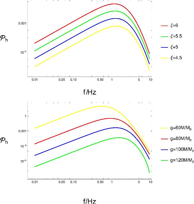
Figure 1. Power spectrum of the field χ for Φ0 = 4.57 Mp when Φ just cross Φ0. Top: we fix g = 100 M/Mp with different ξ. Bottom: we fix ξ = 5 with different g. p0 = a0H0 denotes the scale exiting the horizon at the time when Φ = Φ0. |
In the following we investigate the parameters ξ and g. First, we need to account for the backreaction of particle production on the evolution of the Universe. As mentioned in [18], excessive particle production during inflation can terminate inflation prematurely, failing to provide sufficient e-folding to resolve the flatness problem. In Appendix , we present how the backreaction was considered and equations of perturbations. With backreaction, the effective potential is given by 9 ), we can derive an upper limit on particle produced during inflation. In table 1, we present maximum values of ξ for the given values of g. As expected, larger g allows for larger ξ.
$\begin{eqnarray}\begin{array}{r}{V}_{{\rm{eff}}}=V(\phi )+\frac{1}{2}{g}^{2}{(\phi -{\phi }_{0})}^{2}\left\langle {\chi }^{2}\right\rangle .\end{array}\end{eqnarray}$
The condition to prevent inflation from ending prematurely is: $\begin{eqnarray}\begin{array}{r}\frac{{\rm{d}}{V}_{{\rm{eff}}}}{{\rm{d}}\phi }={g}^{2}\left(\phi -{\phi }_{0}\right)\left\langle {\chi }^{2}\right\rangle +\frac{{\rm{d}}V}{{\rm{d}}\phi }\geqslant 0.\end{array}\end{eqnarray}$
From equation (Table 1. The corresponding maximum value of ξ for different g when Φ0 = 5.42 Mp. |
| g M/Mp | 20 | 40 | 60 | 80 | 100 | 120 | 140 | 160 | 180 | 200 |
|---|---|---|---|---|---|---|---|---|---|---|
| ξ | 0.57 | 0.94 | 1.27 | 1.58 | 1.86 | 2.14 | 2.4 | 2.65 | 2.89 | 3.13 |
To estimate the effects on CMB B-Mode polarization, we need to identify the values of g and ξ which can induce the strongest GWs at the CMB scale. We calculate the energy spectrum of GWs at CMB scale k = 0.05 Mpc−1. We find g ≈ 160 M/Mp, ξ ≈ 2.65 can induce the strongest GWs at CMB scale k = 0.05 Mpc−1.
In figures 2 and 3, we present the resulting energy spectrum of the GWs signal and the total energy spectrum of GWs including the standard primordial one and the particles induced one. The spectrum features a peak around the CMB scale, consistent with our requirements. Through comparison with vacuum GWs, we reveal that even the peak value is only about 0.3% of that of the vacuum GWs. Compared with the results in [18], the GWs obtained under both conditions exhibit similar single-peak waveforms, but their ratio to primordial GWs differs by more than 104. The maximum peak value of the resulting GWs energy spectrum is on the order of 10−23, which is unobservable by any prospective GW experiment [27–29] or CMB B-Mode polarization experiment [9–12] and makes no detectable contribution to the effective number of neutrinos ΔNeff [30–34].
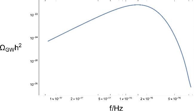
Figure 2. The energy spectrum of induced GWs with Φ0 = 5.42 M/Mp, g = 160 M/Mp, ξ = 2.65. |
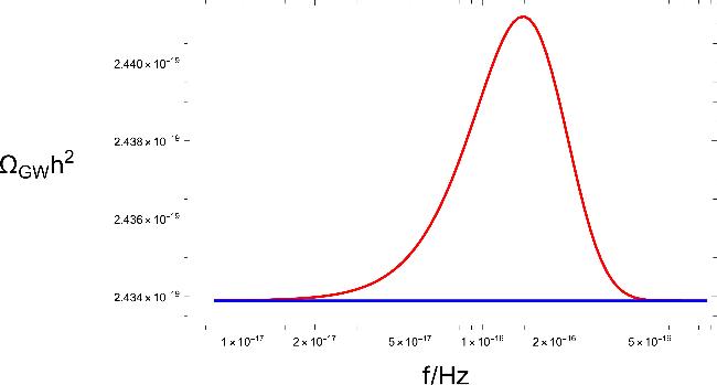
Figure 3. The total energy spectrum of GWs including the vacuum GWs and the particles induced one. The blue line represents the standard vacuum GWs predicted by the Starobinsky potential, and the red line is the total energy spectrum of GWs. |
3.2. Impact on scalar spectral index
In this section, we will study the effect of backreaction on the scalar spectral index and compare the results with observational data.
In Appendix , we present the equations to calculate the first-order curvature perturbation ${ \mathcal R }$. Utilizing these equations, we calculate the scalar spectral index ns and the tensor-to-scalar ratio r, finding ns = 0.966 541, r = 0.003 067 27 at N = 60 and observe a significant increase in ns, which forms a bulge at N < 60 with the parameters we given earlier. The observed increase in the spectral index ns can be attributed to the production of particles. When Φ crosses Φ0, the effective potential becomes flat, resulting in an increase in ns. To investigate this further, we select two representative values of Φ0 and vary the particle numbers by adjusting ξ. In Figure 4, we present the ns–r plane for various parameters along with the constraints on ns derived from the P + ACT + LB + BK18 results [19]. Notably, we find that certain parameter selections yield a scalar spectral index that falls within the 1σ confidence region.
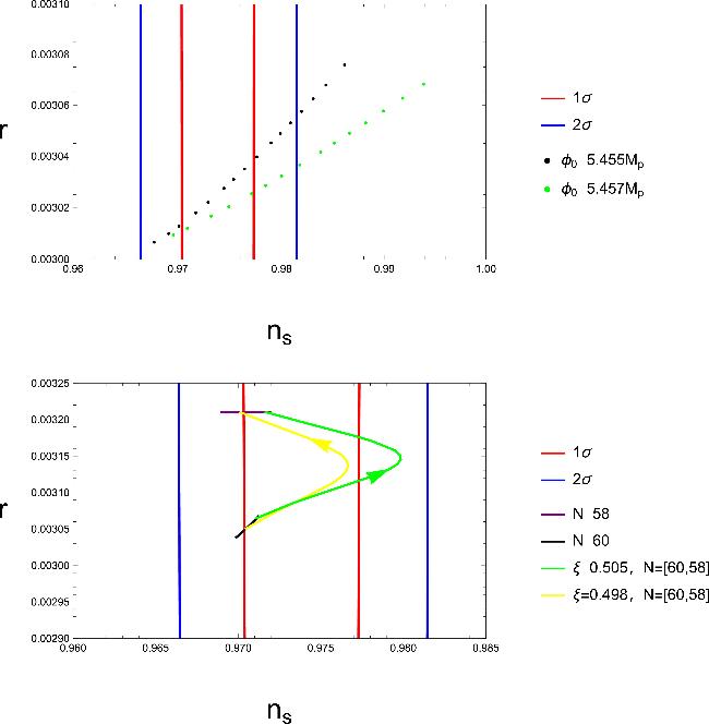
Figure 4. Prediction of our model with constraints on the scalar and tensor primordial power spectra according to ACT at N = 60, shown in the r–ns parameter space. Top: we fix parameter g = 160 M/Mp and change particle numbers through adjusting the value of ξ from 1.4 to 2.65. Bottom: we fix Φ0 = 5.5 Mp, g = 18 M/Mp and change particle numbers through adjusting the value of ξ from 0.49 to 0.505. The yellow and blue lines corresponds to the number of e-folding of inflation N = [60, 58] with ξ = 0.498, ξ = 0.505 respectively, where N = [60, 58] corresponds to the duration of correction of particle production. The arrow denotes the direction of evolution. |
In the calculation for the top panel of Figure 4, we found that the effects of ns still can only last for a short period. Therefore, we reduce the values of g to prolong the duration of particle production and modified Φ0 to ensure that particle production occurs at the desired time. The results indicate that our model can significantly correct the scalar spectral index ns and the predictions of some values of parameters fall within the 1σ confidence region. Furthermore, after accounting for the constraints imposed by backreaction on the parameters, the influence of the produced particle can guarantee scalar spectral index ns remains within the 1σ confidence region for approximately two e-folding numbers of inflation. The process of particle production is expected to persist for approximately one Hubble time, and the backreaction on the Universe will sustain about 1–2 e-folds. Consequently, the spectral index ns is anticipated to increase by approximately 2–3 e-folds. However, in this scenario, the characteristic peak of the induced GWs shifts to larger scales, and the contribution of the produced particles to the total power spectrum of GWs at CMB scales becomes negligible.
In Figure 5, we show the prediction of the scalar spectral index ns and its running ${\rm{d}}{n}_{{\rm{s}}}/{\rm{d}}\mathrm{ln}k$ with constraints on them derived from the P + ACT + LB result [20]. The particle number density rapidly decreases due to the expansion of the Universe. This resulting in a sharp decline in ${\rm{d}}{n}_{{\rm{s}}}/{\rm{d}}\mathrm{ln}k$. Therefore, at the end of particle production, the prediction of ${\rm{d}}{n}_{{\rm{s}}}/{\rm{d}}\mathrm{ln}k$ lies outside the 2σ confidence interval, which lasts about 1 e-fold.
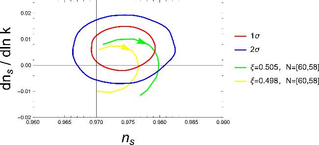


Figure 5. Prediction of the scalar spectral index ns and its running ${\rm{d}}{n}_{{\rm{s}}}/{\rm{d}}\mathrm{ln}k$. The green and yellow lines correspond to the lines of identical colors in Figure 4. |
The results indicate that, given the constraints on ns driven by P + ACT + LB + BK18, the particles generated through this process are unlikely to produce significant GWs and will have a negligible correction on the tensor-to-scalar ratio r, on the order of 10−5. As such, it cannot be detected by any prospective CMB B-mode polarization experiment [9–12]. Therefore, we can ignore the effects of the produced scalar particles on CMB B-mode polarization. The impact on ns is more worthy of attention. After accounting for the backreaction from the produced particles, Φ will oscillate around Φ0 [18] which could leave a noteworthy correction to the scalar spectral index ns. Since the order of the power spectrum remains unchanged, the tensor-to-scalar ratio r does not exhibit any observable variation. As shown in the bottom panel of Figure 4, the predictions of the Starobinsky inflation model can return to within the 1σ confidence region given by ACT for certain parameter values. Obviously, such a phenomenon is not confined to this specific inflation model; thus, when comparing the predictions of various inflation models with observational data, it is essential to consider the production of particles during the inflationary phase.
4. Conclusion and discussion
In this paper, we examined the parameters governing particle production in the nonminimally coupled model and the GWs induced by the produced particles. The parameters g and ξ, which serve as coupling constants in this model, determine the duration over which particles are copiously produced. The parameter Φ0 sets the time at which this process begins and influences the characteristic frequency of the scalar field χ. Then we verified these analyzes by numerical calculations. Through the analysis of equation (2), we infer that induced GWs will feature a peak near the characteristic frequency of χ. By selecting an appropriate value for Φ0, we ensured that the induced GWs produced a peak close to the CMB scale, which allowed us to assess the impact of these particles on the detection of primordial GWs.
Taking into account the backreaction of particle production on inflation, we have identified specific values for g and ξ that generate the strongest GWs at the CMB scale without violating the slow-roll mechanism. However, even for extreme values of g and ξ, the power spectrum of the induced GWs only reaches about 0.3% of that of the vacuum GWs at their peak. It means the induced GWs are unobservable by any prospective GW experiment and CMB B-Mode polarization experiment.
When we take the constraints on ns driven by P + ACT + LB + BK18 data set, we observed that the induced GWs become negligible. However, the impact of our model on ns is significant. It can correct the prediction of the Starobinsky inflation model back to fall within the 1σ confidence region driven by P + ACT + LB + BK18 result in some cases. This phenomenon can also be found in other inflation model, so it is significant to consider the impact on ns from particles produced during inflation when combining theoretical predictions with observational data.
Appendix The basic equations with backreaction of perturbations
In this section, we briefly review the basic equations with backreation of perturbations given by [18]. The spatially flat FRW metric in the conformal Newtonian gauge reads:
$\begin{eqnarray}\begin{array}{r}{\rm{d}}{s}^{2}=-\left(1+2{\rm{\Psi }}\right){\rm{d}}{t}^{2}+{a}^{2}\left[\left(1-2{\rm{\Psi }}\right){\delta }_{ij}+{h}_{ij}^{(1)}+\frac{{h}_{ij}}{2}\right]{\rm{d}}{x}^{i}{\rm{d}}{x}^{j},\end{array}\end{eqnarray}$
where the $\Psi$, ${h}_{ij}^{(1)}$ and hij are the first-order scalar metric perturbation, the first-order tensor perturbation, and the second-order tensor perturbation, respectively. The first-order curvature perturbation is given by $\begin{eqnarray}\begin{array}{r}{{ \mathcal R }}_{{\boldsymbol{k}}}={{\rm{\Psi }}}_{{\boldsymbol{k}}}+\frac{H\delta {\phi }_{{\boldsymbol{k}}}}{\dot{\phi }}.\end{array}\end{eqnarray}$
Incorporating Hartree terms into the equation of motion, the background equations read: $\begin{eqnarray}\begin{array}{rcl}3{M}_{{\rm{p}}}^{2}{H}^{2} & = & \frac{1}{1+\xi {M}_{{\rm{p}}}^{-2}\left\langle {\chi }^{2}\right\rangle }\left[\frac{1}{2}{\dot{\phi }}^{2}+\frac{1}{2}\left\langle \delta {\dot{\phi }}^{2}\right\rangle \right.\\ & & +\frac{1}{2}\left\langle {\dot{\chi }}^{2}\right\rangle +\frac{1}{2{a}^{2}}\left\langle {({\rm{\nabla }}\delta \phi )}^{2}\right\rangle +\frac{1}{2{a}^{2}}\left\langle {({\rm{\nabla }}\chi )}^{2}\right\rangle \\ & & -6\xi H\left\langle \chi \dot{\chi }\right\rangle +\frac{\xi }{{a}^{2}}\left\langle {{\rm{\nabla }}}^{2}({\chi }^{2})\right\rangle +V(\phi )\\ & & \left.+\frac{1}{2}\frac{{\partial }^{2}V}{\partial {\phi }^{2}}\left\langle \delta {\phi }^{2}\right\rangle +\frac{1}{2}{g}^{2}{\left(\phi -{\phi }_{0}\right)}^{2}\left\langle {\chi }^{2}\right\rangle \right],\end{array}\end{eqnarray}$
$\begin{eqnarray}\begin{array}{rcl}-{M}_{{\rm{p}}}^{2}\left(2\dot{H}+3{H}^{2}\right) & = & \frac{1}{1+\xi {M}_{{\rm{p}}}^{-2}\left\langle {\chi }^{2}\right\rangle }\left[\frac{1}{2}{\dot{\phi }}^{2}+\frac{1}{2}\left\langle \delta {\dot{\phi }}^{2}\right\rangle \right.\\ & & +\left(\frac{1}{2}+2\xi \right)\left\langle {\dot{\chi }}^{2}\right\rangle -\frac{1}{6{a}^{2}}\left\langle {({\rm{\nabla }}\delta \phi )}^{2}\right\rangle \\ & & -\frac{1}{6{a}^{2}}\left\langle {({\rm{\nabla }}\chi )}^{2}\right\rangle -\frac{2\xi }{3{a}^{2}}\left\langle {{\rm{\nabla }}}^{2}({\chi }^{2})\right\rangle \\ & & +4\xi H\left\langle \chi \dot{\chi }\right\rangle +2\xi \left\langle \chi \ddot{\chi }\right\rangle -V(\phi )\\ & & \left.-\frac{1}{2}\frac{{\partial }^{2}V}{\partial {\phi }^{2}}\left\langle \delta {\phi }^{2}\right\rangle -\frac{1}{2}{g}^{2}{\left(\phi -{\phi }_{0}\right)}^{2}\left\langle {\chi }^{2}\right\rangle \right],\end{array}\end{eqnarray}$
$\begin{eqnarray}\begin{array}{r}\ddot{\phi }+3H\dot{\phi }+\frac{\partial V}{\partial \phi }+\frac{1}{2}\frac{{\partial }^{3}V}{\partial {\phi }^{3}}\left\langle \delta {\phi }^{2}\right\rangle +{g}^{2}\left(\phi -{\phi }_{0}\right)\left\langle {\chi }^{2}\right\rangle =0.\end{array}\end{eqnarray}$
Then, the momentum-space linearized field perturbation equations are given by $\begin{eqnarray}\begin{array}{r}\delta {\ddot{\phi }}_{{\boldsymbol{k}}}+3H\delta {\dot{\phi }}_{{\boldsymbol{k}}}+{{\rm{\Omega }}}_{{\boldsymbol{k}}}^{2}\delta {\phi }_{{\boldsymbol{k}}}=4{\dot{{\rm{\Psi }}}}_{{\boldsymbol{k}}}\dot{\phi }-2\frac{\partial V}{\partial \phi }{{\rm{\Psi }}}_{{\boldsymbol{k}}},\end{array}\end{eqnarray}$
$\begin{eqnarray}\begin{array}{r}{\ddot{\chi }}_{{\boldsymbol{k}}}+3H{\dot{\chi }}_{{\boldsymbol{k}}}+{\omega }_{{\boldsymbol{k}}}^{2}{\chi }_{{\boldsymbol{k}}}=0,\end{array}\end{eqnarray}$
with $\begin{eqnarray}\begin{array}{r}{{\rm{\Omega }}}_{{\boldsymbol{k}}}^{2}=\frac{{k}^{2}}{{a}^{2}}+\frac{{\partial }^{2}V}{\partial {\phi }^{2}}+{g}^{2}\left\langle {\chi }^{2}\right\rangle +\frac{1}{2}\frac{{\partial }^{4}V}{\partial {\phi }^{4}}\left\langle \delta {\phi }^{2}\right\rangle ,\end{array}\end{eqnarray}$
$\begin{eqnarray}\begin{array}{r}{\omega }_{{\boldsymbol{k}}}^{2}=\frac{{k}^{2}}{{a}^{2}}+{g}^{2}{\left(\phi -{\phi }_{0}\right)}^{2}+{g}^{2}\left\langle \delta {\phi }^{2}\right\rangle -6\xi \left({\dot{H}}^{2}+2{H}^{2}\right),\end{array}\end{eqnarray}$
and the perturbed Einstein equations is $\begin{eqnarray}\begin{array}{r}3H{\dot{{\rm{\Psi }}}}_{{\boldsymbol{k}}}+\left(\frac{{k}^{2}}{{a}^{2}}+3{H}^{2}\right){{\rm{\Psi }}}_{{\boldsymbol{k}}}=-\frac{1}{2{M}_{{\rm{p}}}^{2}}\left(\dot{\phi }\delta {\phi }_{{\boldsymbol{k}}}-{{\rm{\Psi }}}_{{\boldsymbol{k}}}{\dot{\phi }}^{2}+\frac{{\rm{d}}V}{{\rm{d}}\phi }\delta {\phi }_{{\boldsymbol{k}}}\right),\end{array}\end{eqnarray}$
$\begin{eqnarray}\begin{array}{r}{\dot{{\rm{\Psi }}}}_{{\boldsymbol{k}}}+H{{\rm{\Psi }}}_{{\boldsymbol{k}}}=\frac{\dot{\phi }}{2{M}_{{\rm{p}}}^{2}}\delta {\phi }_{{\boldsymbol{k}}}.\end{array}\end{eqnarray}$
Using (A10 ) and (A11 ), we can obtain $\Psi$k as
$\begin{eqnarray}\begin{array}{r}{{\rm{\Psi }}}_{{\boldsymbol{k}}}=\frac{\dot{\phi }\delta {\dot{\phi }}_{{\boldsymbol{k}}}+3H\dot{\phi }\delta {\phi }_{{\boldsymbol{k}}}+(\partial V/\partial \phi )\delta {\phi }_{{\boldsymbol{k}}}}{{\dot{\phi }}^{2}-2{M}_{{\rm{p}}}^{2}{\left(k/a\right)}^{2}}.\end{array}\end{eqnarray}$
The equation of motion for the first-order tensor perturbation ${h}_{ij}^{(1)}$ and second-order tensor perturbation hij is given by
$\begin{eqnarray}\begin{array}{r}{h}_{ij}^{(1)^{\prime\prime} }(\tau ,{\boldsymbol{x}})+2{ \mathcal H }{h}_{ij}^{(1)^{\prime} }(\tau ,{\boldsymbol{x}})-{{\rm{\nabla }}}^{2}{h}_{ij}^{(1)}(\tau ,{\boldsymbol{x}})=0,\end{array}\end{eqnarray}$
$\begin{eqnarray}\begin{array}{r}{h}_{ij}^{{\prime\prime} }(\tau ,{\boldsymbol{x}})+2{ \mathcal H }{h}_{ij}^{{\prime} }(\tau ,{\boldsymbol{x}})-{{\rm{\nabla }}}^{2}{h}_{ij}(\tau ,{\boldsymbol{x}})=\frac{4}{{M}_{{\rm{p}}}^{2}}{\pi }_{ij}^{TT}(\tau ,{\boldsymbol{x}}),\end{array}\end{eqnarray}$
where a prime denotes the derivative with respect to the conformal time τ ≡ ∫tdt/a, and ${ \mathcal H }\equiv {a}^{{\prime} }/a$ denotes the conformal Hubble parameter. The power spectrum, ${{ \mathcal P }}_{h}={\sum }_{\lambda =+,\times }{k}^{3}/(2{\pi }^{2})| {h}_{{\boldsymbol{k}}}^{\lambda }{| }^{2}$, has the following form $\begin{eqnarray}\begin{array}{r}{{ \mathcal P }}_{h}(k)=\frac{2{k}^{3}}{{\pi }^{4}{M}_{{\rm{p}}}^{4}}{\displaystyle \int }_{0}^{\pi }{\rm{d}}\theta {\sin }^{5}\theta \displaystyle \int {\rm{d}}p{p}^{6}{\left|{\displaystyle \int }^{\tau }{\rm{d}}{\tau }^{{\prime} }{G}_{{\boldsymbol{k}}}\left(\tau ,{\tau }^{{\prime} }\right){\chi }_{{\boldsymbol{p}}}{\chi }_{| {\boldsymbol{k}}-{\boldsymbol{p}}| }\right|}^{2},\end{array}\end{eqnarray}$
where $\begin{eqnarray}\begin{array}{r}{h}_{ij}=\displaystyle \sum _{\lambda =+,\times }\displaystyle \int \frac{{\rm{d}}{{\boldsymbol{k}}}^{3}}{{(2\pi )}^{3/2}}{{\rm{e}}}^{{\rm{i}}{\boldsymbol{k}}\cdot {\boldsymbol{x}}}{{\rm{e}}}_{ij}^{\lambda }({\boldsymbol{k}}){h}_{{\boldsymbol{k}}}^{\lambda }(\tau ),\end{array}\end{eqnarray}$
$\begin{eqnarray}\begin{array}{rcl}{G}_{{\boldsymbol{k}}}\left(\tau ,{\tau }^{{\prime} }\right) & = & \frac{1}{{k}^{3}{\tau }^{{\prime} 2}}\left[\left(1+{k}^{2}\tau {\tau }^{{\prime} }\right)\sin k(\tau -{\tau }^{{\prime} })\right.\\ & & \left.-k(\tau -{\tau }^{{\prime} })\cos k(\tau -{\tau }^{{\prime} })\right]{\rm{\Theta }}(\tau -{\tau }^{{\prime} }).\end{array}\end{eqnarray}$
$\begin{eqnarray}\begin{array}{rc}{\pi }_{ij}^{TT} & =\displaystyle \sum _{\lambda =+,\times }\displaystyle \int \frac{{\rm{d}}{{\boldsymbol{k}}}^{3}{\rm{d}}{{\boldsymbol{p}}}^{3}}{{(2\pi )}^{3}}{{\rm{e}}}^{{\rm{i}}{\boldsymbol{k}}\cdot {\boldsymbol{x}}}{{\rm{e}}}_{ij}^{\lambda }{e}^{\lambda ,lm}{p}_{l}{p}_{m}{\chi }_{| {\boldsymbol{k}}-{\boldsymbol{p}}| }{\chi }_{p}.\end{array}\end{eqnarray}$