

1. Introduction
Resistor network models are applied across a wide range of disciplines, in addition to electrical problems, they also exist in non-electrical, biological, synthetic chemistry, optical issues, and more. Examples include using circuit networks to simulate chaotic quantum billiards [1], linear circuit designs and simulations [2], modeling the electrical properties of 3D printed grids using resistor lattice theory [3], the path multiplicity in ER random networks [4], research and application of lattice Green’s function, etc [5–7].
It is well known that calculating the electric potential function and the effective resistance of a resistor network is a challenging task. This is particularly difficult for arbitrarily large-scale finite resistor networks, as any change in the network structure affects the solution for electrical characteristics. In fact, boundary conditions impose strong constraints, influencing computational methods and procedures. Consequently, solving every complex network issue requires innovative ideas and creative methods [8].
Reviewing the history of resistor network (RN) research, the initial, relatively mature circuit theory can be traced back to the two fundamental circuit laws established by Kirchhoff in 1845. This theory can solve a series of small-scale circuit problems [8]. Some 150 years later, in the year 2000, Cserti utilized Green’s function techniques to study infinite RNs [5]. Subsequent applications solved some new problems [9–11], but this Green’s function technique is not suitable for calculating finite lattices. To address the problems of finite RNs, F. Y. Wu proposed the Laplacian matrix method (LM) in 2004 [12]. This method has important applications [13–16], but it is not applicable to lattices with arbitrary boundary conditions. In 2011 [8], established an innovative theory for studying arbitrary resistor network models (RNMs), now called Tan’s recursion-transform (RT) theory [16]. The advantage of the RT theory is that the established matrix equation depends only on matrices in one direction. It has solved RNMs with various complex structures [17–30]. The current RT theory is subdivided into two forms: one is the method using current parameters to establish the matrix equation [19–25], abbreviated as the RT-I method; the other is the method using node voltage parameters to establish the matrix equation [26–30], abbreviated as the RT-V method. Generally, both methods are suitable for studying RNMs with arbitrary boundary conditions. The series of papers in [31–37] re-explore the series network models in [17–29] using the RT theory, propose some optimization methods, and provide another expression form.
Research indicates that a special Möbius-strip (MS) network model exists in nature. An MS is a ring-shaped topological figure with an 180° twist in its band, resulting in only one surface (single-sided). It was first proposed by August Ferdinand Möbius (1790–1868) in the 19th century. For centuries, the MS, with its unique 180° twisted ring, has motivated philosophers, scientists, and artists, and will continue to prompt thought and exploration of such models. For example, in 2022, the teams of Yasutomo Segawa and Kenichiro Itami at Nagoya University, successfully synthesized a Möbius carbon nanobelt and isolated and characterized it [38]. Reference [39] studied an FeSn alloy with a Möbius shape, successfully developing a highly twisted, C-wrapped 3D graded porous FeSn integrated anode.
In summary, the study of RNMs involves multiple disciplines, and the MS network model (MSNM) is a valuable research topic, perhaps with more existence and value to be discovered in future research. This paper intends to research a versatile m × n MSNM, as shown in Figure 1. The study of its electrical characteristic formula has been challenging enough for over a hundred years. Although [12] provided a resistance formula expressed in double summation in 2004, our research aims to directly obtain the potential and resistance results expressed in a single summation. The unit cells in Figure 1 can be resistors, or RLC circuits composed of inductors and capacitors. For calculation purposes, the elements within the unit cell can simply be denoted by r and r1 (r and r1 represent not only resistors but also RLC circuit elements or fractional- order circuit elements [40, 41]). This research will achieve theoretical and methodological innovation, providing analytical expressions for the electric potential function and effective resistance in single summation.
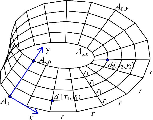
Figure 1. An arbitrary m × n MS network model, where m (mark s = m-1) and n refer to the number of nodes in the longitudinal and periodic directions, respectively. The unit resistor on the Y-axis is r1, and the unit resistor on the axis along the periodic direction is r. |
2. Two main conclusions
2.1. Analytical expression of potential function
Consider an arbitrary m × n MS circuit network model as shown in Figure 1, where m denotes the number of nodes along the Y-axis (e.g., ${A}_{0,k}{A}_{s,k}$ axis), n denotes the number of nodes along the periodic (cyclic) direction. The impedance element on the Y-axis is r1, and the unit impedance on the axis along the periodic direction is r. Selecting ${A}_{0}(0,0)$ as the origin of the Cartesian coordinate system, the voltage parameter at any node $d(x,y)$ is denoted as ${V}_{x}^{(y)}$(${V}_{m\times n}(x,y)$, refer to the circuit model in Figure 2). Consider current J is input at ${d}_{1}({x}_{1},{y}_{1})$ and output at ${d}_{2}({x}_{2},{y}_{2})$, and selecting $\displaystyle {\sum }_{i=0}^{m-1}{V}_{0}^{(i)}=0$ as the reference voltage, then the electric potential function at any node $d(x,y)$ for an arbitrary m×n MSNM is
$\begin{eqnarray}\begin{array}{l}{V}_{m\times n}\left(x,y\right)=\displaystyle \frac{rJ}{m}\left(x\displaystyle \frac{{x}_{2}-{x}_{1}}{n}-\left({x}_{k}-{x}_{1}\right)\right)\\ \,+\,\displaystyle \frac{2rJ}{m}\displaystyle \sum _{i=1}^{m-1}\displaystyle \frac{{P}_{{x}_{1}-x}^{(i)}{C}_{{y}_{1},i}-{P}_{{x}_{2}-x}^{(i)}{C}_{{y}_{2},i}}{{b}_{i}^{n}+{\bar{b}}_{i}^{n}-{\left(-1\right)}^{i}2}{C}_{y,i},\end{array}\end{eqnarray}$
where ${x}_{k}$, ${C}_{y,i}$ and ${F}_{k}^{(i)}$ are defined as $\begin{eqnarray}{x}_{k}=\left\{\begin{array}{c}{x}_{1},\,{\rm{if}}\,{x}_{k}\leqslant {x}_{1}\\ x,\,{\rm{if}}\,{x}_{1}\leqslant {x}_{k}\leqslant {x}_{2}\\ {x}_{2},\,{\rm{if}}\,{x}_{k}\geqslant {x}_{2}\end{array}\right.,\end{eqnarray}$
$\begin{eqnarray}{C}_{{y}_{k},i}=\,\cos \left({y}_{k}+\displaystyle \frac{1}{2}\right){\phi }_{i},\,{\phi }_{i}=i\pi /m,\end{eqnarray}$
$\begin{eqnarray}\begin{array}{l}{P}_{{x}_{1}-x}^{(i)}={F}_{n-\left|{x}_{1}-x\right|}^{(i)}+{\left(-1\right)}^{i}{F}_{\left|{x}_{1}-x\right|}^{(i)},\,\\ {F}_{k}^{(i)}=\left({b}_{i}^{k}-{\bar{b}}_{i}^{k}\right)/\left({b}_{i}-{\bar{b}}_{i}\right),\end{array}\end{eqnarray}$
meanwhile $q=r/{r}_{1}$, and $\begin{eqnarray}\begin{array}{lll}{b}_{i} & = & q+1-q\,\cos \,{\phi }_{i}+\sqrt{{(q+1-q\,\cos \,{\phi }_{i})}^{2}-1,}\\ {\bar{b}}_{i} & = & q+1-q\,\cos \,{\phi }_{i}-\sqrt{{(q+1-q\,\cos \,{\phi }_{i})}^{2}-1.}\end{array}\end{eqnarray}$
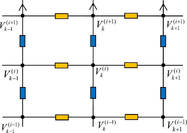
Figure 2. A sub-network model with resistor elements and node potential parameters. |
2.2. Equivalent resistance analytical formula
Considering a class of arbitrary m × n MSNM shown in Figure 1, the analytical expression for the effective resistance between any node ${d}_{1}({x}_{1},{y}_{1})$ and ${d}_{2}({x}_{2},{y}_{2})$ is4 ).
$\begin{eqnarray}\begin{array}{c}{R}_{m\times n}\left({d}_{1},{d}_{2}\right)=\displaystyle \frac{r}{m}\left|{x}_{2}-{x}_{1}\right|\left(1-\displaystyle \frac{\left|{x}_{2}-{x}_{1}\right|}{n}\right)\\ \,+\,\displaystyle \frac{2r}{m}\displaystyle \sum _{i=1}^{m-1}\displaystyle \frac{{F}_{n}^{(i)}({C}_{1,i}^{2}+{C}_{2,i}^{2})-2{P}_{{x}_{1}-{x}_{2}}^{(i)}{C}_{1,i}{C}_{2,i}}{{b}_{i}^{n}+{\bar{b}}_{i}^{n}-{(-1)}^{i}2},\end{array}\end{eqnarray}$
where ${\phi }_{i}=i\pi /m$, and ${C}_{k,i}$ (k = 1,2) is the abbreviation for ${C}_{{y}_{k},i}$, and ${F}_{k}^{(i)}$ is defined in equation (The above two main conclusions (1) and (6) are presented for the first time in this article and belong to the original research results. The following is the derivation process for the above conclusion.
3. Proof of main conclusions
The current advanced theory for studying arbitrary resistor network models is the RT-V theory established in [26] in 2017. Subsequent studies [27–30] further enriched the RT-V theory. This article further develops the RT-V theory and divides it into five main steps (see the 5 steps below), among which the matrix transformation step varies due to different network structures, especially the network structure in this article which is different from a series of previous models, and the matrix transformation requires mathematical innovation. This article will derive the conclusions proposed in the previous section based on the basic steps of the RT-V theory.
Step 1. Establish the main matrix equation. Referring to the circuit model in Figure 2, without considering the constraints of current input and output, a discrete Laplace two-dimensional equation $({{\rm{\Delta }}}_{x}^{2}+h{{\rm{\Delta }}}_{y}^{2}){V}_{x}^{(y)}=0$ can be established based on the node voltage equation theory ($\displaystyle \sum {r}_{i}^{-1}{V}_{k}=0$), assuming $q=r/{r}_{1}$, then
$\begin{eqnarray}\begin{array}{l}{V}_{k+1}^{(0)}=(2+q){V}_{k}^{(0)}-{V}_{k-1}^{(0)}-q{V}_{k}^{(1)},\,i=0\\ {V}_{k+1}^{(i)}=(2+2q){V}_{k}^{(i)}-{V}_{k-1}^{(i)}-q{V}_{k}^{(i-1)}-q{V}_{k}^{(i+1)},\,1\leqslant i\lt m\\ {V}_{k+1}^{(m-1)}=(2+q){V}_{k}^{(m-1)}-{V}_{k-1}^{(m-1)}-q{V}_{k}^{(m-2)},\,i=m-1\end{array}\end{eqnarray}$
If considering that current J is input from node ${d}_{1}({x}_{1},{y}_{1})$ and output from node ${d}_{2}({x}_{2},{y}_{2})$, a constraint equation related to current input and output can be established. This constraint equation, together with equation (7 ), can be written as a unified matrix equation
$\begin{eqnarray}{\mathop{V}\limits^{ \rightharpoonup }}_{k+1}={A}_{m\times m}{\mathop{V}\limits^{ \rightharpoonup }}_{k}-{\mathop{V}\limits^{ \rightharpoonup }}_{k-1}-rJ({\delta }_{i,{y}_{1}}{\delta }_{k,{x}_{1}}-{\delta }_{i,{y}_{2}}{\delta }_{k,{x}_{2}}),\end{eqnarray}$
where ${\delta }_{k,x}$ is the Dirac symbol, and $\begin{eqnarray}{\mathop{V}\limits^{ \rightharpoonup }}_{k}={\left[{V}_{k}^{(0)}\,{,}\,{V}_{k}^{(1)}\,{,}\,{V}_{k}^{(2)}\,{,}\,\cdots \,{,}\,{V}_{k}^{\left(m-1\right)}\right]}^{T},\end{eqnarray}$
and ${A}_{m\times m}$ is a $m\times m$ matrix, it is a tridiagonal matrix $\begin{eqnarray}{A}_{m\times m}=\left(\begin{array}{lllll}2+q & -q & 0 & 0 & 0\\ -q & 2\left(1+q\right) & -q & 0 & 0\\ & \vdots & \ddots & \vdots & \\ 0 & 0 & -q & 2\left(1+q\right) & -q\\ 0 & 0 & 0 & -q & 2+q\end{array}\right).\end{eqnarray}$
Step 2. Establish the boundary condition matrix equation. The boundary here refers to the area with the Y-axis as the boundary, where the surface undergoes a 180 degree flip at this position, resulting in the network always having only one face. Establish a discrete matrix difference equation based on the theory of the node voltage equation10 ), while ${D}_{m\times m}$ is a reverse identity matrix, which is11 ) and (12 ) show the cyclicality and periodicity along the horizontal direction, where equation (13 ) expresses the flipping characteristics of the interface.
$\begin{eqnarray}{\mathop{V}\limits^{ \rightharpoonup }}_{1}={A}_{m\times m}{\mathop{V}\limits^{ \rightharpoonup }}_{0}-{D}_{m\times m}{\mathop{V}\limits^{ \rightharpoonup }}_{n-1},\end{eqnarray}$
$\begin{eqnarray}{\mathop{V}\limits^{ \rightharpoonup }}_{n}={D}_{m\times m}{\mathop{V}\limits^{ \rightharpoonup }}_{0},\end{eqnarray}$
where the matrix ${A}_{m\times m}$ is given by equation ( $\begin{eqnarray}{D}_{m\times m}=\left(\begin{array}{cc}\begin{array}{cc}0 & 0\\ 0 & 0\end{array} & \begin{array}{cc}\cdots 0 & 1\\ \cdots 1 & 0\end{array}\\ \begin{array}{cc}\vdots & \unicode{x022F0}\\ 1 & 0\end{array} & \begin{array}{cc}\vdots & \vdots \\ \cdots 0 & 0\end{array}\end{array}\right).\end{eqnarray}$
Equations (Equations (7 )–(13 ) are all the equations we need to derive the electric potential function. However, it is impossible for people to directly solve these 2D systems of equations, which is an important technical challenge. To solve this difficulty, we have created new matrix transform techniques while applying the RT theory. Next, we will first present the methods of the matrix transform, and then provide their general and specific solutions.
Step 3. Reduce the dimension of the equation through matrix transform. The series of equations established above are all 2D equations. Here, matrix transform techniques are used to reduce these 2D equations to 1D difference equations. Firstly, the eigenvalue ${p}_{i}$ of the tridiagonal matrix ${A}_{m\times m}$ can be solved using the determinant $\det \left|{A}_{m}-p{E}_{m}\right|=0\,{,}$ 8 )15 ) and let it be an identity. After a series of algebraic operations, obtain8 ) and performing the transform, we can obtain11 ) and (12 ), we obtain20 ) and (21 ) above is the original technique of this article (first implementation), and it is precisely this technological breakthrough that can effectively derive the analytical formula proposed earlier in the article.
$\begin{eqnarray}{p}_{i}=2(1+q)-2q\,\cos \,{\phi }_{i},\end{eqnarray}$
and ${\phi }_{i}=i\pi /m$ $(i=0,1,2,\cdots m-1)$. Next, design an undetermined square matrix ${B}_{m\times m}$ and perform the following matrix transform on matrix ${A}_{m\times m}$ in 2D equation ( $\begin{eqnarray}{B}_{m\times m}{A}_{m\times m}={\rm{diag}}\{{p}_{0},{p}_{1},\cdots ,{p}_{m-1}\}{B}_{m\times m}.\end{eqnarray}$
Expand equation ( $\begin{eqnarray}{B}_{m\times m}=\left(\begin{array}{ll}\begin{array}{cc}1/\sqrt{2} & 1/\sqrt{2}\\ \cos \left(\displaystyle \frac{1}{2}\right){\phi }_{1} & \cos \left(1+\displaystyle \frac{1}{2}\right){\phi }_{1}\end{array} & \begin{array}{cc}\cdots & 1/\sqrt{2}\\ \cdots & \cos \left(m-\displaystyle \frac{1}{2}\right){\phi }_{1}\end{array}\\ \begin{array}{cc}\vdots & \vdots \\ \cos \left(\displaystyle \frac{1}{2}\right){\phi }_{m-1} & \cos \left(1+\displaystyle \frac{1}{2}\right){\phi }_{m-1}\end{array} & \begin{array}{cc}\ddots & \vdots \\ \cdots & \cos \left(m-\displaystyle \frac{1}{2}\right){\phi }_{m-1}\end{array}\end{array}\right).\end{eqnarray}$
At the same time, its inverse matrix can be obtained $\begin{eqnarray}{B}_{m\times m}^{-1}=\displaystyle \frac{2}{m}{B}_{m\times m}^{T}.\end{eqnarray}$
Therefore, by left multiplying the matrix ${B}_{m\times m}$ by the matrix equation ( $\begin{eqnarray}{X}_{k+1}^{(i)}={p}_{i}{X}_{k}^{(i)}-{X}_{k-1}^{(i)}-rJ\left({\delta }_{{x}_{1},k}{C}_{{y}_{1},i}-{\delta }_{{x}_{2},k}{C}_{{y}_{2},i}\right),\end{eqnarray}$
where according to matrix (16), ${C}_{y,i}=\,\cos \left(y+\displaystyle \frac{1}{2}\right){\phi }_{i}$ ($i\geqslant 1$), ${C}_{y,0}=1/\sqrt{2}$ are obtained, and the following transformation relationship exists $\begin{eqnarray}{\mathop{X}\limits^{ \rightharpoonup }}_{k}={B}_{m+1}{\mathop{V}\limits^{ \rightharpoonup }}_{k},\,{\mathop{X}\limits^{ \rightharpoonup }}_{k}={\left[{X}_{k}^{(0)}\,{,}\,{X}_{k}^{(1)}\,{,}\,\cdots \,{,}\,{X}_{k}^{(m)}\right]}^{{\rm{T}}}.\end{eqnarray}$
Similarly, by multiplying matrix ${B}_{m\times m}$ by the boundary condition matrix equations ( $\begin{eqnarray}{X}_{1}^{(i)}={p}_{i}{X}_{0}^{(i)}-{(-1)}^{i}{X}_{n-1}^{(i)},\end{eqnarray}$
$\begin{eqnarray}{X}_{n}^{(i)}={(-1)}^{i}{X}_{0}^{(i)},\,(i=0,1,2,\,\cdots m),\end{eqnarray}$
The transformation of equations (Step 4. Solve the difference equation system. The above equations (18 ), (20 ), and (21 ) are 1D difference equations, and their general and specific solutions can be solved based on the theory and techniques in [28]. We need to solve it in segments here, that is, consider two cases of $i=0$ and $i\geqslant 1$ respectively.
Firstly, consider $i=0\Rightarrow {\phi }_{0}=0$, and ${p}_{0}=2$, which is a special eigenvalue. After a series of algebraic operations, solve the above equations (18 ), (20 ), and (21 ) to derive the following results ($0\leqslant k\leqslant n$)2 )), and ${X}_{0}^{(0)}$ is an undetermined initial value that can be determined using a reference potential value.
$\begin{eqnarray}{X}_{k}^{(0)}={X}_{0}^{(0)}+\left(k\displaystyle \frac{{x}_{2}-{x}_{1}}{n}-({x}_{k}-{x}_{1})\right)\displaystyle \frac{rJ}{\sqrt{2}},\end{eqnarray}$
where ${x}_{k}$ is a piecewise function ${x}_{k}=\left\{{x}_{1}:{x}_{k}\leqslant {x}_{1}\right\}\cup $ $\left\{x:\,{x}_{1}\leqslant {x}_{k}\leqslant {x}_{2}\right\}\cup \left\{{x}_{2}:{x}_{k}\geqslant {x}_{2}\right\}$ (this is the same expression as equation (Using the transformation ${\mathop{X}\limits^{ \rightharpoonup }}_{k}={B}_{m+1}{\mathop{V}\limits^{ \rightharpoonup }}_{k}$ in equation (19 ), ${X}_{0}^{(0)}=\displaystyle \frac{1}{\sqrt{2}}\displaystyle {\sum }_{i=0}^{m-1}{V}_{0}^{(i)}$ is derived. Since the potential is a relative value, its zero potential point can be assumed arbitrarily, so $\displaystyle {\sum }_{i=0}^{m-1}{V}_{0}^{(i)}=0$ can be assumed, simplifying equation (22 ).
Next, considering the case of $i\geqslant 1$, after a series of algebraic operations using equations (14 )–(21 ), the solution can be obtained3 ) and (4 ), respectively.
$\begin{eqnarray}\displaystyle \frac{{X}_{k}^{(i)}}{rJ}=\displaystyle \frac{{P}_{{x}_{1}-k}^{(i)}{C}_{{y}_{1},i}-{P}_{{x}_{2}-k}^{(i)}{C}_{{y}_{2},i}}{{b}_{i}^{n}+{\bar{b}}_{i}^{n}-{(-1)}^{i}2},\end{eqnarray}$
where ${C}_{y,i}$ and ${F}_{k}^{(i)}$ are defined in equations (Step 5. Use the matrix inverse transform to calculate the node potential and equivalent resistance. By using equation (19 ), its inverse transformation ${\mathop{V}\limits^{ \rightharpoonup }}_{k}={[{B}_{m\times m}]}^{-1}{\mathop{X}\limits^{ \rightharpoonup }}_{k}$ can be obtained, and by applying equation (17 ), it can be written as22 ) and (23 ) into equation (24 ) yields the analytical equation (1 ) for the potential function proposed earlier.
$\begin{eqnarray}{V}_{k}^{(y)}=\displaystyle \frac{2}{m}\left(\displaystyle \frac{1}{\sqrt{2}}{X}_{k}^{(0)}+\displaystyle \sum _{i=1}^{m-1}{X}_{k}^{(i)}\cos (y+\displaystyle \frac{1}{2}){\phi }_{i}\right).\end{eqnarray}$
Substituting equations (Next, according to Ohm’s law, calculate the resistance: ${R}_{m\times n}({d}_{1},{d}_{2})\,=$ $\displaystyle \frac{1}{J}[V({x}_{1},{y}_{1})-V({x}_{2},{y}_{2})]$, and obviously, the node voltage needs to be calculated first. For example, using equation (1 ) to obtain analytical expressions for node voltages ${V}_{m\times n}({x}_{1},{y}_{1})$ and ${V}_{m\times n}({x}_{2},{y}_{2})$, respectively6 ) can be derived.
$\begin{eqnarray}\begin{array}{c}{V}_{m\times n}\left({x}_{1},{y}_{1}\right)=\displaystyle \frac{rJ}{m}\left(\displaystyle \frac{{x}_{2}-{x}_{1}}{n}\right){x}_{1}\\ \,+\,\displaystyle \frac{2rJ}{m}\displaystyle \sum _{i=1}^{m-1}\displaystyle \frac{{F}_{n}^{(i)}{C}_{{y}_{1},i}-{P}_{{x}_{2}-{x}_{1}}^{(i)}{C}_{{y}_{2},i}}{{b}_{i}^{n}+{\bar{b}}_{i}^{n}-{(-1)}^{i}2}{C}_{{y}_{1},i},\end{array}\end{eqnarray}$
$\begin{eqnarray}\begin{array}{c}{V}_{m\times n}\left({x}_{2},{y}_{2}\right)=\displaystyle \frac{rJ}{m}\left({x}_{2}\displaystyle \frac{{x}_{2}-{x}_{1}}{n}-({x}_{2}-{x}_{1})\right)\\ \,+\,\displaystyle \frac{2rJ}{m}\displaystyle \sum _{i=1}^{m-1}\displaystyle \frac{{P}_{{x}_{2}-{x}_{1}}^{(i)}{C}_{{y}_{1},i}-{F}_{n}^{(i)}{C}_{{y}_{2},i}}{{b}_{i}^{n}+{\bar{b}}_{i}^{n}-{(-1)}^{i}2}{C}_{{y}_{2},i}.\end{array}\end{eqnarray}$
By substituting them into the ${R}_{m\times n}({d}_{1},{d}_{2})\,=$ $\displaystyle \frac{1}{J}[V({x}_{1},{y}_{1})-V({x}_{2},{y}_{2})]$ calculation, equation (Thus, the two main conclusions (1) and (6) proposed in the article have been proven, and all the equations and calculations mentioned above are rigorous and self-consistent. As mentioned earlier, the unit cell structure in Figure 1 is not only applicable to RNs, but also to complex impedance and fractional order circuits [40, 41]. The following discusses the special cases and applications of electric potential and resistance formula.
4. Discussion of results
4.1. Visualization of potential function
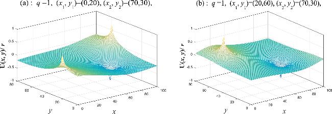
Figure 3. The potential function diagram under the same conditions for node d2 but different conditions for d1, where (n, m) = (100, 80): (a) the nodes are d1 (0, 20) and d2 (70, 30) respectively; (b) the nodes are d1(20, 60) and d2(70, 30) respectively. |
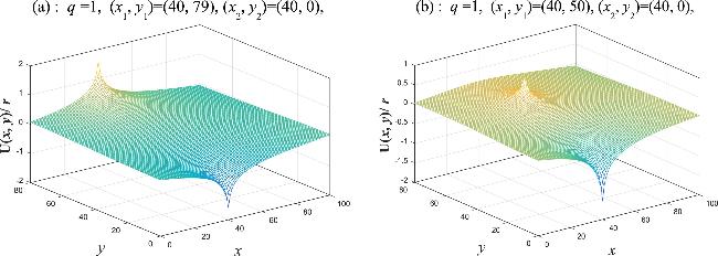
Figure 4. The potential function diagram under the same conditions for node d2 but different conditions for d1 where (n, m) = (100, 80): (a) the nodes are d1(40, 79) and d2(40, 0) respectively; (b) the nodes are d1(40, 50) and d2(40, 0) respectively. |
In the four potential function graphs of figures 3 and 4, a positive peak appears at node d1 for current input, and a negative peak appears at node d2 for current output. However, two positive peaks appear in Figure 3(a) because their positions are actually the same node, solely due to the distorted 180° periodic structure. For example, for MSNM with (n, m) = (100, 80), node d1 (0, y) is actually node d’1 (100, 79-y), which means that node d1 (0, 20) and d’1 (100, 59) are two overlapping nodes.
4.2. Visualization of equivalent resistance
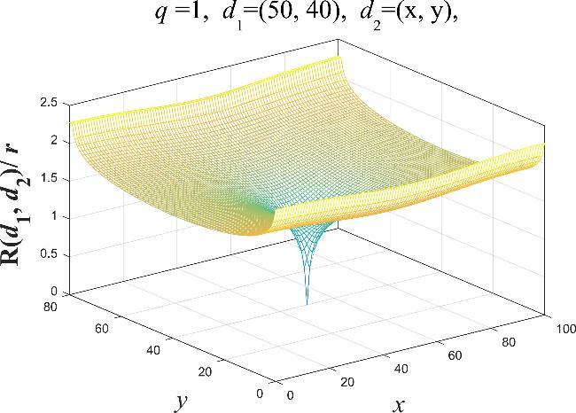
Figure 5. Visualization of equivalent resistance, let (n, m) = (100, 80), using d1 (50, 40) as the fixed point and d2(x, y) as the moving point. |
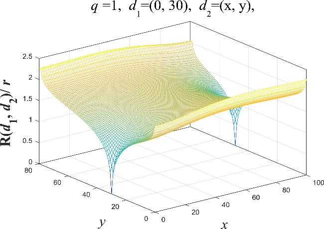
Figure 6. Visualization of equivalent resistance, let (n, m) = (100, 80), using d1 (0, 30) as the fixed point and d2(x, y) as the moving point. |
In the image of Figure 5, take (n, m) = (100, 80), if a fixed point d1 (50, 40) is taken, when the changing node d2 (x, y) moves to the d1 position, the resistance between the two nodes d2 and d1 is zero (a minimum value appears in the image). The equivalent resistance relationship of all positions forms a funnel structure.
In Figure 6, when fixed point d1 (0, 30) is taken, two minimum values appear in the graph, it is because node d1 (0, 30) and node d’1 (100, 50) are actually two overlapping nodes (due to cycle and boundary flipping). Therefore, when the changing node d2 (x, y) moves to position d1, the resistance between its two nodes d2 and d1 must be zero.
4.3. Discussion of potential function
The analytical formula (1 ) for the electric potential is a general expression, and for the convenience of readers’ understanding, a series of special results are considered below.
Case 1: in the electric potential equation (1 ), if ${x}_{2}={x}_{1}$, then the electric potential of any node $d(x,y)$ of m × n order MSNM is3 ) and (4 ), respectively.
$\begin{eqnarray}{V}_{m\times n}\left(x,y\right)=\displaystyle \frac{2rJ}{m}\displaystyle \sum _{i=1}^{m-1}\displaystyle \frac{{P}_{{x}_{1}-x}^{(i)}({C}_{{y}_{1},i}-{C}_{{y}_{2},i})}{{b}_{i}^{n}+{\bar{b}}_{i}^{n}-{(-1)}^{i}2}{C}_{y,i},\end{eqnarray}$
where ${C}_{y,i}$ and ${F}_{k}^{(i)}$ are defined in equations (Case 2: in the potential function equation (1 ), assuming ${x}_{1}=0$, the potential function of arbitrary node $d(x,y)$ in the m × n order MSNM is2 )–(4 ), respectively.
$\begin{eqnarray}\begin{array}{c}{V}_{m\times n}(x,y)=\displaystyle \frac{rJ}{m}\left(x\displaystyle \frac{{x}_{2}}{n}-{x}_{k}\right)\\ \,+\,\displaystyle \frac{2rJ}{m}\displaystyle \sum _{i=1}^{m-1}\displaystyle \frac{{P}_{x}^{(i)}{C}_{{y}_{1},i}-{P}_{{x}_{2}-x}^{(i)}{C}_{{y}_{2},i}}{{b}_{i}^{n}+{\bar{b}}_{i}^{n}-{(-1)}^{i}2}{C}_{y,i},\end{array}\end{eqnarray}$
where ${x}_{k}$, ${C}_{y,i}$ and ${F}_{k}^{(i)}$ are defined in equations (Case 3: in the potential function equation (1 ), if ${y}_{2}={y}_{1}$, then the potential function of any node $d(x,y)$ is
$\begin{eqnarray}\begin{array}{l}{V}_{m\times n}\left(x,y\right)=\displaystyle \frac{rJ}{m}\left(x\displaystyle \frac{{x}_{2}-{x}_{1}}{n}-\left({x}_{k}-{x}_{1}\right)\right)\\ \,+\,\displaystyle \frac{2rJ}{m}\displaystyle \sum _{i=1}^{m-1}\displaystyle \frac{{P}_{{x}_{1}-x}^{(i)}-{P}_{{x}_{2}-x}^{(i)}}{{b}_{i}^{n}+{\bar{b}}_{i}^{n}-{(-1)}^{i}2}{C}_{{y}_{1},i}{C}_{y,i}.\end{array}\end{eqnarray}$
Case 4: in the potential function equation (1 ), let ${y}_{1}\,=0,{y}_{2}=m-1$, then ${C}_{0,i}=\,\cos \left(\displaystyle \frac{1}{2}{\phi }_{i}\right)$, ${C}_{{y}_{2},i}={(-1)}^{i}{C}_{0,i}$, the potential function of any node $d(x,y)$ of m × n order MSNM is
$\begin{eqnarray}\begin{array}{l}{V}_{m\times n}(x,y)=\displaystyle \frac{rJ}{m}\left(x\displaystyle \frac{{x}_{2}-{x}_{1}}{n}-\left({x}_{k}-{x}_{1}\right)\right)\\ \,+\,\displaystyle \frac{2rJ}{m}\displaystyle \sum _{i=1}^{m-1}\displaystyle \frac{{P}_{{x}_{1}-x}^{(i)}-{\left(-1\right)}^{i}{P}_{{x}_{2}-x}^{\left(i\right)}}{{b}_{i}^{n}+{\bar{b}}_{i}^{n}-{\left(-1\right)}^{i}2}{C}_{0,i}{C}_{y,i}.\end{array}\end{eqnarray}$
4.4. Discussion of equivalent resistance
Formula (6 ) is a universal conclusion that applies to all situations. For example, $0\leqslant n\leqslant \infty $, $0\leqslant m\leqslant \infty $, $0\leqslant \{{x}_{1},{x}_{2}\}\leqslant n$, $0\leqslant \{{y}_{1},{y}_{2}\}\leqslant m-1$. To help readers further analyze the physical meaning of formula (6 ), some special conclusions are given below.
Case 5: considering any m × n order MSNM in Figure 1, when ${d}_{1}=(0,{y}_{1})$, ${d}_{2}=(x,{y}_{2})$, the resistance formula (6 ) degenerates into
$\begin{eqnarray}\begin{array}{c}{R}_{m\times n}\left({d}_{1},{d}_{2}\right)=\displaystyle \frac{rx}{m}\left(1-\displaystyle \frac{x}{n}\right)\\ \,+\,\displaystyle \frac{2r}{m}\displaystyle \sum _{i=1}^{m-1}\displaystyle \frac{{F}_{n}^{(i)}\left({C}_{1,i}^{2}+{C}_{2,i}^{2}\right)-2{P}_{x}^{(i)}{C}_{1,i}{C}_{2,i}}{{b}_{i}^{n}+{\bar{b}}_{i}^{n}-{\left(-1\right)}^{i}2}.\end{array}\end{eqnarray}$
Case 6: considering any m × n order MSNM in Figure 1, when ${d}_{1}=(x,{y}_{1})$, ${d}_{2}=(x,{y}_{2})$, the resistance formula (6 ) reduces to32 ) degenerates into
$\begin{eqnarray}{R}_{m\times n}\left({d}_{1},{d}_{2}\right)=\displaystyle \frac{2r}{m}\displaystyle \sum _{i=1}^{m-1}\displaystyle \frac{{F}_{n}^{(i)}{({C}_{1,i}-{C}_{2,i})}^{2}}{{b}_{i}^{n}+{\bar{b}}_{i}^{n}-{(-1)}^{i}2}.\end{eqnarray}$
Specifically, if ${x}_{1}={x}_{2}$ and considering ${y}_{1}=0$ and ${y}_{2}\,=m-1$, then formula ( $\begin{eqnarray}{R}_{m\times n}\left({d}_{1},{d}_{2}\right)=\displaystyle \frac{4r}{m}\displaystyle \sum _{i=1}^{m-1}\displaystyle \frac{{F}_{n}^{(i)}[1-{\left(-1\right)}^{i}]}{{b}_{i}^{n}+{\bar{b}}_{i}^{n}-{(-1)}^{i}2}{\cos }^{2}\left(\displaystyle \frac{1}{2}{\phi }_{i}\right).\end{eqnarray}$
Case 7: when ${d}_{1}=(0,0)$ and ${d}_{2}=(x,0)$, the resistance formula (6 ) reduces to
$\begin{eqnarray}\begin{array}{c}{R}_{m\times n}\left({d}_{1},{d}_{2}\right)\,=\displaystyle \frac{r}{m}x\left(1-\displaystyle \frac{x}{n}\right)\\ \,+\,\displaystyle \frac{4r}{m}\displaystyle \sum _{i=1}^{m-1}\displaystyle \frac{{F}_{n}^{(i)}-{P}_{x}^{(i)}}{{b}_{i}^{n}+{\bar{b}}_{i}^{n}-{(-1)}^{i}2}{\cos }^{2}\left(\displaystyle \frac{1}{2}{\phi }_{i}\right).\end{array}\end{eqnarray}$
Case 8: considering $n\to \infty $ but m and ${x}_{2}-{x}_{1}$ are finite values, the network in this case is a semi-infinite network, which can be obtained by taking the limit $n\to \infty $ from formula (6 )
$\begin{eqnarray}\begin{array}{c}{R}_{m\times \infty }({d}_{1},{d}_{2})=\displaystyle \frac{\left|{x}_{2}-{x}_{1}\right|}{m}r\\ \,+\,\displaystyle \frac{r}{m}\displaystyle \sum _{i=1}^{m-1}\displaystyle \frac{{C}_{1,i}^{2}+{C}_{1,i}^{2}-{\bar{\lambda }}_{i}^{\left|{x}_{2}-{x}_{1}\right|}{C}_{1,i}{C}_{2,i}}{\sqrt{{(1+q-q\,\cos \,{\theta }_{i})}^{2}-1}}.\end{array}\end{eqnarray}$
Case 9: when m = 2, the model in Figure 1 degenerates into a simple n-order MS resistor network model, see Figure 7. At this point, ${\phi }_{1}=\pi /2$, the unit resistance on the periodic boundary is r, and the unit resistance on the short axis (Y-axis) is r1, $q=r/{r}_{1}$. By substituting into equation (5 ), we obtain ${b}_{1}=1+q+\sqrt{q\left(q+2\right)}$, ${\bar{b}}_{1}=1+q-\sqrt{q\left(q+2\right)}$. Therefore, from equation (6 ), we obtain ($0\leqslant x\leqslant n$)36 ) and (37 ) here, which verifies the correctness of the theoretical formula derived in the article.
$\begin{eqnarray}{R}_{n}({A}_{0},{B}_{x})=\displaystyle \frac{r}{2}x\left(1-\displaystyle \frac{x}{n}\right)+r\left(\displaystyle \frac{{F}_{n}^{(1)}+{F}_{n-x}^{(1)}-{F}_{x}^{(1)}}{{b}_{1}^{n}+{\bar{b}}_{1}^{n}+2}\right),\end{eqnarray}$
$\begin{eqnarray}{R}_{n}({A}_{0},{A}_{x})=\displaystyle \frac{r}{2}x\left(1-\displaystyle \frac{x}{n}\right)+r\left(\displaystyle \frac{{F}_{n}^{(1)}-{F}_{n-x}^{(1)}+{F}_{x}^{(1)}}{{b}_{1}^{n}+{\bar{b}}_{1}^{n}+2}\right).\end{eqnarray}$
Reference [42] specifically studied the problem of Case 9, and the conclusions derived are identical to the conclusions in (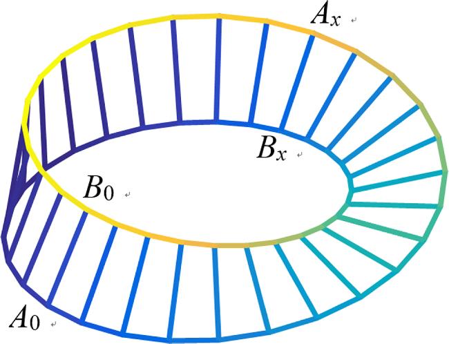


Figure 7. An arbitrary n-order MSNM, where A0 is the coordinate origin, and Ax and Bx are any nodes on two axis. |
5. Comparison and validation
As a byproduct of our research, we discovered a new mathematical identity during comparative studies. Referring to the network model in Figure 1 [12], first studied the equivalent resistance of any m × n order MSNM, selecting ${A}_{0}(0,0)$ as the origin of the Cartesian coordinate system. The analytical formula for the equivalent resistance given in [12] is
$\begin{eqnarray}\begin{array}{c}{R}_{m\times n}({d}_{1},{d}_{2})=\displaystyle \frac{r}{m}\left(\left|{x}_{1}-{x}_{2}\right|-\displaystyle \frac{{\left({x}_{1}-{x}_{2}\right)}^{2}}{n}\right)\\ \,+\,\displaystyle \frac{1}{nm}\displaystyle \sum _{j=0}^{n-1}\displaystyle \sum _{i=1}^{m-1}\displaystyle \frac{{C}_{1}^{2}+{C}_{2}^{2}-2{C}_{1}{C}_{2}\,\cos \left[\left({x}_{1}-{x}_{2}\right)\left(4j+1-{(-1)}^{i}\right)\displaystyle \frac{\pi }{2n}\right]}{{r}^{-1}\left[1-\,\cos \left(4j+1-{\left(-1\right)}^{i}\right)\displaystyle \frac{\pi }{2n}\right]+{r}_{1}^{-1}\left(1-\,\cos \,{\phi }_{i}\right)},\end{array}\end{eqnarray}$
where ${C}_{1}=\,\cos \left({y}_{1}+\displaystyle \frac{1}{2}\right){\phi }_{i}$, ${C}_{2}=\,\cos \left({y}_{2}+\displaystyle \frac{1}{2}\right){\phi }_{i}$ and ${\phi }_{i}\,=i\pi /m$.Formula (38 ) is a double summation expression derived using the LM method established by F. Y. Wu [12], which can be referred to as a 2D result. People always hope to reduce this 2D result to a 1D calculation result, but this is a challenging task. For example [13], the dimensionality reduction calculation when m = 2 (only m = 2) was specifically studied, and needed to consider the discussion of n = odd and n = even separately. Obviously, the dimensionality reduction of identity equations is a very difficult task.
The equivalent resistance analytical formula (6 ) in this article is the result given by the single summation expression using the RT-V theory. The two equivalent resistances derived from the same network model must be equal. Obviously, our results can conveniently reduce the 2D result of formula (38 ) to a 1D result, which is a meaningful discovery. From this, we discovered a new mathematical identity, and based on the equality between formula (6 ) and formula (38 ), we can then obtain the below.
Proposition: Given that m, n are natural numbers, and $q\gt 0$, $0\leqslant {x}_{i}\leqslant n-1$, $0\leqslant {y}_{i}\leqslant m-1$, ${\phi }_{i}=i\pi /m$, ${C}_{k}=\,\cos \left({y}_{k}+\displaystyle \frac{1}{2}\right){\phi }_{i}$, , and ${F}_{k}^{(i)}$ and ${P}_{x}^{(i)}$ are defined in equation (4 ), ${b}_{k}$ and ${\bar{b}}_{k}$ are defined in equation (5 ), then there is an identity equation:
$\begin{eqnarray}\begin{array}{c}\displaystyle \frac{1}{2n}\displaystyle \sum _{j=0}^{n-1}\displaystyle \sum _{i=1}^{m-1}\displaystyle \frac{{C}_{1}^{2}+{C}_{2}^{2}-2{C}_{1}{C}_{2}\,\cos \left[\left({x}_{1}-{x}_{2}\right)\left(4j+1-{\left(-1\right)}^{i}\right)\displaystyle \frac{\pi }{2n}\right]}{\left[1-\,\cos \left(4j+1-{\left(-1\right)}^{i}\right)\displaystyle \frac{\pi }{2n}\right]+q\left(1-\,\cos \,{\phi }_{i}\right)}\\ \,=\,\displaystyle \sum _{i=1}^{m-1}\displaystyle \frac{{F}_{n}^{(i)}\left({C}_{1}^{2}+{C}_{2}^{2}\right)-2{P}_{{x}_{2}-{x}_{1}}^{(i)}{C}_{1}{C}_{2}}{{b}_{i}^{n}+{\bar{b}}_{i}^{n}-{(-1)}^{i}2}.\end{array}\end{eqnarray}$
This is a new mathematical identity that reduces a double sum to a single sum (reducing 2D operations to 1D calculations). It is easy for people to use computer programming to verify its correctness. By using this identity, many interesting new identities can be derived. Below are its four corollaries.Inference 1: if $m=2$, ${x}_{1}=0$, ${x}_{2}=x$ (natural numbers) in formula (39 ), then ${\phi }_{1}=\pi /2$. At this point, identity (39) degenerates into
$\begin{eqnarray}\begin{array}{l}\displaystyle \frac{1}{2n}\displaystyle \sum _{j=0}^{n-1}\displaystyle \frac{{C}_{1}^{2}+{C}_{2}^{2}-2{C}_{1}{C}_{2}\,\cos \left[x\left(2j+1\right)\tfrac{\pi }{n}\right]}{q+1-\,\cos \left(2j+1\right)\tfrac{\pi }{n}}\\ \,=\displaystyle \frac{{F}_{n}^{(1)}\left({C}_{1}^{2}+{C}_{2}^{2}\right)-2\left({F}_{n-x}^{(1)}-{F}_{x}^{(1)}\right){C}_{1}{C}_{2}}{{b}_{1}^{n}+{\bar{b}}_{1}^{n}+2},\end{array}\end{eqnarray}$
where ${F}_{k}^{(i)}=({b}_{i}^{k}-{\bar{b}}_{i}^{k})/({b}_{i}-{\bar{b}}_{i})$, and ($q\gt 0$), $\begin{eqnarray}{b}_{1}=q+1+\sqrt{{q}^{2}+2q},\,{\bar{b}}_{1}=q+1-\sqrt{{q}^{2}+2q}.\end{eqnarray}$
Inference 2: if ${y}_{2}={y}_{1}=0$ in formula (40 ), then ${C}_{2}={C}_{1}=\,\cos \left(\displaystyle \frac{\pi }{4}\right)$ $=\sqrt{2}/2$. At this point, identity (40 ) degenerates into42 ) is denoted as H, then we obtain,42 ) is an identity.
$\begin{eqnarray}\displaystyle \frac{1}{2n}\displaystyle \sum _{j=0}^{n-1}\displaystyle \frac{1-\,\cos \left[x(2j+1)\tfrac{\pi }{n}\right]}{q+1-\,\cos (2j+1)\tfrac{\pi }{n}}=\displaystyle \frac{{F}_{n}^{(1)}-{F}_{n-x}^{(1)}+{F}_{x}^{(1)}}{{b}_{1}^{n}+{\bar{b}}_{1}^{n}+2}.\end{eqnarray}$
One can simply verify its correctness. For example, if $x=0$ and the identity equation ( $\begin{eqnarray}\begin{array}{rcl}H(\mathrm{left}) & = & \displaystyle \frac{1}{2n}\displaystyle \sum _{j=0}^{n-1}\displaystyle \frac{1-\,\cos (0)}{q+1-\,\cos (2j+1)\tfrac{\pi }{n}}=0,\\ H(\mathrm{right}) & = & \displaystyle \frac{{F}_{n}^{(1)}-{F}_{n}^{(1)}+{F}_{0}^{(1)}}{{b}_{1}^{n}+{\bar{b}}_{1}^{n}+2}=0.\end{array}\end{eqnarray}$
Obviously, when $x=0$, equation (Again, if $n=2$, $x=1$, and the identity equation (42 ) is denoted as H, then we obtain,42 ) holds. Of course, one can also use computers to verify the correctness of equation (42 ).
$\begin{eqnarray}\begin{array}{l}H{\left.({\rm{left}})\right|}_{n=2}=\displaystyle \frac{1}{4}\left(\displaystyle \frac{1-\,\cos \left(\displaystyle \frac{\pi }{2}\right)}{q+1-\,\cos \left(\displaystyle \frac{\pi }{2}\right)}+\displaystyle \frac{1-\,\cos \left(\displaystyle \frac{3\pi }{2}\right)}{q+1-\,\cos \left(\displaystyle \frac{3\pi }{2}\right)}\right)=\displaystyle \frac{1}{2(q+1)} & ,\\ H{\left.({\rm{right}})\right|}_{n=2}=\displaystyle \frac{{F}_{2}^{(1)}-{F}_{1}^{(1)}+{F}_{1}^{(1)}}{{b}_{1}^{2}+{\bar{b}}_{1}^{2}+2}=\displaystyle \frac{1}{2(q+1)}.\end{array}\end{eqnarray}$
Obviously, when $n=2$ and $x=1$, the identity equation (Inference 3: if ${x}_{1}={x}_{2}$ in formula (39 ), then identity equation (39 ) degenerates into
$\begin{eqnarray}\begin{array}{c}\displaystyle \frac{1}{2n}\displaystyle \sum _{j=0}^{n-1}\displaystyle \sum _{i=1}^{m-1}\displaystyle \frac{{({C}_{1}-{C}_{2})}^{2}}{\left[1-\,\cos (4j+1-{(-1)}^{i})\displaystyle \frac{\pi }{2n}\right]+q(1-\,\cos \,{\phi }_{i})}\\ \,=\,\displaystyle \sum _{i=1}^{m-1}\displaystyle \frac{{F}_{n}^{(i)}{({C}_{1}-{C}_{2})}^{2}}{{b}_{i}^{n}+{\bar{b}}_{i}^{n}-{(-1)}^{i}2}.\end{array}\end{eqnarray}$
Inference 4: if the natural numbers ${y}_{1}={y}_{2}=y$, ${x}_{1}=0$, ${x}_{2}=x$ and ${\phi }_{i}=i\pi /m$, then the identity equation (39 ) degenerates into
$\begin{eqnarray}\begin{array}{c}\displaystyle \frac{1}{n}\displaystyle \sum _{j=0}^{n-1}\displaystyle \sum _{i=1}^{m-1}\displaystyle \frac{\left\{1-\,\cos \left[x(4j+1-{(-1)}^{i})\displaystyle \frac{\pi }{2n}\right]\right\}{\cos }^{2}\left[\left(y,+,\displaystyle \frac{1}{2}\right){\phi }_{i}\right]}{\left[1-\,\cos (4j+1-{(-1)}^{i})\displaystyle \frac{\pi }{2n}\right]+q(1-\,\cos \,{\phi }_{i})}\\ \,=\,2\displaystyle \sum _{i=1}^{m-1}\displaystyle \frac{{F}_{n}^{(i)}-[{F}_{n-x}^{(i)}+{(-1)}^{i}{F}_{x}^{(i)}]}{{b}_{i}^{n}+{\bar{b}}_{i}^{n}-{(-1)}^{i}2}{\cos }^{2}\left[\left(y,+,\displaystyle \frac{1}{2}\right){\phi }_{i}\right].\end{array}\end{eqnarray}$
The above identities are all given for the first time in this article and are by-products discovered incidentally, which establishes a new fundamental theory for algebra in the field of mathematics. The above identities have been calculated and verified by computers. At this point, we have mutually verified the results of [12] with our own results.
6. Comments and prospects
The article first uses the RT-V theory to research the arbitrary MS network model, further developing the RT-V theory established in [26], and establishing new matrix equation (11 )~(13 ), cleverly transforming the 2D matrix equations in the article into 1D equations. This is the first time that a single summation expression has been proposed for the electric potential and effective resistance of any m × n MSNM.
The variation of the potential function with coordinate parameters under different conditions was plotted using Matlab drawing tools, revealing the influence of the current input and output positions on the potential of any node. The variation of equivalent resistance with coordinate parameters under different conditions was plotted, revealing the influence of the coordinate positions of two nodes on equivalent resistance. The MS network model is an interesting mathematical model and an important physical model that has appeared in scientific research fields [38, 39]. The research work in this article can provide new theoretical value for related research work, as well as new research thinking for related researchers.