The Navier–Stokes (NS) equation with Coriolis force and density-dependent viscosity is an important physical model, which has been widely used to understand and analyze a wide array of phenomena, including behaviors of the Gulf stream, dynamics of hurricanes, operation of chemical reactors and functionality of rotating machines. In this paper, based on the matrix and curve integration techniques, we build a sufficient condition for the existence of Cartesian vector solutions u = b(t) + A(t)x for the N-dimensional NS equation, in which A satisfies appropriate matrix equations. Then, we discuss two special cases of A and thereby explicit analytical solutions are obtained. To shed light on these solutions, we give some illustrative examples. Among them, some examples form the generalization previously obtained by other authors and some examples are quite new. Finally, we analyze the properties of Cartesian vector solutions in a special case.
Hongli An, Ziliang Li, Anthony Suen, Manwai Yuen. On the compressible Navier–Stokes equation with Coriolis force and density-dependent viscosity: the Cartesian vector solutions and their properties[J]. Communications in Theoretical Physics, 2026, 78(5): 055001. DOI: 10.1088/1572-9494/ae3381
1. Introduction
In the present work, our main concern is with derivation of Cartesian vector solutions for the compressible Navier–Stokes equation with Coriolis force and density-dependent viscosity, which takes the following form [1]:
where ${\boldsymbol{x}}={({x}_{1},{x}_{2},\cdots ,\,{x}_{N})}^{{\rm{T}}}\in {R}^{N}$ is the spatial coordinate, J is an antisymmetric matrix arising from the Coriolis force, ρ(x, t), u(x, t) and p(x, t) denote the density, velocity and pressure of the fluid, respectively. While,
The Navier–Stokes equation has drawn extensive scientific interest being the cornerstone in modelling fluids, plasmas, astrophysics, oceanography and atmospheric dynamics [2–4]. In particular, the Navier–Stokes (NS) equation with Coriolis force and density-dependent viscosity has exerted a profound influence on the rotational fluid dynamics, which is fundamental to understand and analyze a wide array of phenomena, including the behavior of the Gulf stream, the dynamics of hurricanes, the operation of chemical reactors, the functionality of rotating machines and the intricacies of electrochemical reactors featuring rotating electrodes [5, 6]. Therefore, there have been extensive and intensive studies carried on the NS equation with Coriolis force and different density-dependent viscosity, which is manifested by a large number of related papers [7–15]. For examples, Olshanskii and Reusken investigated numerical solutions to the NS equation with Coriolis force by the robust multigrid method [7]. Codina studied the numerical solutions via the discretization method [8]. Lee and his co-authors derived some analytical solutions for the NS equation with Coriolis force in two dimensions [9]. Yang and his co-authors proved the global existence and uniqueness of weak solutions for the NS equation with the density-dependent viscosity chosen by h(ρ) = 0 and g(ρ) = ξ [10], where ξ is a constant. Mellet and Vasseur showed the existence of weak solutions for the NS equation with h(ρ) = μ and g(ρ) = ξ [11], where μ and ξ are constants. Yuen constructed radially symmetric solutions for the NS equation with h(ρ) = 0 and g(ρ) = κρθ [12]. An and Zhu derived elliptic vortex solutions and pulsrodon solutions for the NS equation with h(ρ) = 0 and g(ρ) = κρθ [13]. Guo and Xin obtained spherically symmetric solutions for the NS equation with h(ρ) = ρθ and g(ρ) = (θ − 1)ρθ [14]. An and Yuen derived drifting solutions for the NS equation with h(ρ) = k1ρθ and g(ρ) = k2ρθ[15].
It is known that in geophysical flows, there are many mathematical models corresponding to (1.1). Among them, the Euler equation descriptive of the motion of inviscid fluids is expressed exactly as (1.1) with h(ρ) = 0 and g(ρ) = 0 [16]. In [17], An and her co-authors have showed that the Euler equation admits the Cartesian vector solutions via the matrix theory and decomposition technique. Subsequently, Chow and his co-authors have proved that the damped Euler equation also admits the Cartesian vector solutions [18]. After that, Fan and Yuen have demonstrated that the Euler equation with Coriolis force admits the Cartesian solutions, too [19]. What needs to be pointed out is that in the Cartesian solutions, the velocity function u(x, t) takes a linear function form of spatial coordinates x. In fact, seeking this type of solution has a long history for fluid flows [20–27], especially for the Euler and NS equations. One of the important results in this direction is the work of Craik and Criminale [28], in which a comprehensive analysis of solutions to the incompressible NS equation was given. Therefore, it is natural to inquire whether the compressible NS equation with Coriolis force and density-dependent viscosity (1.1) admits the general Cartesian vector solutions of this form:
The main goal of this paper is to provide a positive answer to the above question. Here, by using the matrix technique and curve integration technique, we show the existence of general Cartesian vector solutions u = Ax + b(t) for the N-dimensional compressible NS equation (1.1) with the density-dependent viscosity chosen by h(ρ) = k1ρθ and g(ρ) = k2ρθ. These solutions are shown to be global and explicitly expressed by appropriate formulae. In particular, we discuss two special cases on the matrix A wherein some interesting new solutions are obtained. Moreover, the structure and properties of Cartesian vector solutions are discussed in a special case. Based on the importance and applications of the NS equation, the Cartesian vector solutions obtained here may be helpful for experts in understanding how the real fluid will flow and can also provide benchmarks for testing and improving some numerical codes for computing more complicated flows.
The organization of the paper is arranged as follows: In section 2, we show that when the viscosity coefficients are chosen by h(ρ) = k1ρθ and g(ρ) = k2ρθ with θ being a constant, the N-dimensional compressible NS equation (1.1) admits the Cartesian vector solutions wherein A satisfies appropriate matrix equations. To shed light on the solvable cases of the matrix equations, we consider two specials cases of A in sections 3 and 4. In the former, we reveal that when A is an antisymmetric constant matrix and the product of A and J is commutative, the exact rotational solutions can be obtained. In the latter, we show that when A is a time-dependent matrix and J = 0, the exact irrotational solutions can be derived. Meanwhile, some illustrative examples are given for these two solvable cases, which generalize the results obtained in [12, 17, 19, 29]. In section 5, we analyze the structure and properties of Cartesian vector solutions in a special case. Finally, a short conclusion is attached.
2. Existence of the Cartesian vector solutions
For the N-dimensional compressible NS equation (1.1), from the γ-law aspect, we consider the case wherein the density ρ and pressure p satisfy a relation of:
with k > 0 and γ = cp/cu, where cp, cu are the specific heats capacities under constant volume and constant pressure, respectively. In particular, when γ = 1, the fluid is called isothermal. It can be applied to construct models with nondegenerate isothermal cores, which have a role in connection with the so-called Schonberg-Chandrasekhar [30]. When γ = 2, the fluid corresponds to the viscous Saint-Venant system for shallow water [16] and investigated in [14]. When γ = 5/3, 7/5, the equation can describe the dynamics of the monatomic and diatomic gas [5], respectively.
It is noticed from equation (1.1) that we can take k = 1 without loss of generality by using a simple transformation ρ → k−1/γρ, k1 → k1k−1/γ and k2 → k2k−1/γ. Let
with $\mu ={\left(\frac{\gamma -1}{\gamma }\right)}^{\frac{1}{\gamma -1}}$, then the compressible NS equation (1.1) can be readily rewritten into the following form:
Here, for an appropriate function $\bar{p}({\boldsymbol{x}},t)$, our aim is to find a sufficient condition on the existence of the Cartesian vector solutions for the N-dimensional compressible NS equation (2.3), which takes the following form:
In the above, the elements bi(t) and aij(t) (i, j = 1, 2, ⋯ , N) are time-dependent functions. Due to the equivalent relation (2.2) between $\bar{p}$ and ρ, we only need to deal with $\bar{p}$ when solving the equation (2.3). The main results obtained are given in the following theorem:
Here, we shall first prove how to obtain the analytical solutions (2.11) for the compressible NS equation (2.3). Without loss of generality, we shall discuss the case of γ ≠ 1. Substituting (2.10) into the second equation of (2.3) yields:
In order to solve $\bar{p}({\boldsymbol{x}},t)$ through (2.18), these N equations should be compatible with each other, namely, the vector functions (Q1, Q2, ⋯ , QN) should constitute a potential field of $\bar{p}({\boldsymbol{x}},t)$, in which the sufficient and necessary conditions are
This condition means that ${\boldsymbol{C}}=\frac{1}{2}{{\boldsymbol{B}}}^{-1}({{\boldsymbol{A}}}_{t}+{\boldsymbol{JA}}+{{\boldsymbol{A}}}^{2})$ is a symmetric matrix, that is, the condition (2.8) is satisfied.
From the condition (2.19), we can get that the function $\bar{p}({\boldsymbol{x}},t)$ is a complete differential, that is,
Therefore, the second kind of curvilinear integral of $\bar{p}({\boldsymbol{x}},t)$ is independent of its integration route according to the curve integration technique (see references in [31, 32]). This allows us to select a special integration route to get the value of $\bar{p}$:
Next, we shall prove that the functions (2.10)–(2.11) satisfy the first equation of (2.3) under the conditions (2.12) and (2.14). For γ ≠ 1, on inserting (2.9), (2.12) and (2.14) into (2.3)1, we can get
As for the case of γ = 1, it can be proved in a similar way, in which one only needs to replace $\mu {\bar{p}}^{\frac{1}{\gamma -1}}$ with $\exp (\bar{p})$ in the proof procedure of equation (2.22). Therefore, the proof of the existence of analytical Cartesian vector solutions (2.10)–(2.11) for the N-dimensional compressible NS equation (2.3) has been finished. □
We would like to point out that although the condition (2.8)–(2.9) looks simple, it is actually a complicated matrix differential system containing N2 scalar equations. Therefore, it is very difficult to derive its general solutions. In the following, some special techniques are devised to make its analytical solutions obtainable.
It is noticed from (1.1) that when ${\rm{tr}}({\boldsymbol{A}})=0$, the governing equation becomes the incompressible Navier–Stokes equation. However, the result built in theorem 1 still holds. In that case, it reduces to the result given by Craik and Criminale [28]. Also when ${\rm{tr}}({\boldsymbol{A}})=0$ the density is passive and therein it forms a Lagrangian invariant.
In theorem 1, if we set the the Lamé viscosity coefficients k1, k2 to be zero, the Cartesian vector solutions described by (2.10) and (2.11) coincide with the result obtained for the Euler equation [17]. Although the difference between the Euler and Navier–Stokes equations only resides in the two parameters k1 and k2, their intrusion makes the solvable cases for the NS equation much more difficult than that for the Euler equation.
3. The first reduction: constant matrix A
Observation on the form of the matrices B and C in (2.6)–(2.7) inspires us to choose A to be an antisymmetric constant and k1 = 0, which can lead to the rotational Cartesian solutions. The result is built in the following theorem.
If the parameter k1 = 0 and A is a constant matrix satisfying:
With the aid of (3.6) and (3.7), we can directly simplify equations (2.12) and (2.14) into (3.4) and (3.5). The proof is finished. □
It's remarked that by using theorem 2, various special solutions can be obtained for the compressible NS equation when the reduced system is solvable. Here, we give two examples.
For the 2D compressible Navier–Stokes equation with k1 = 0, setting A and J to be the following form:
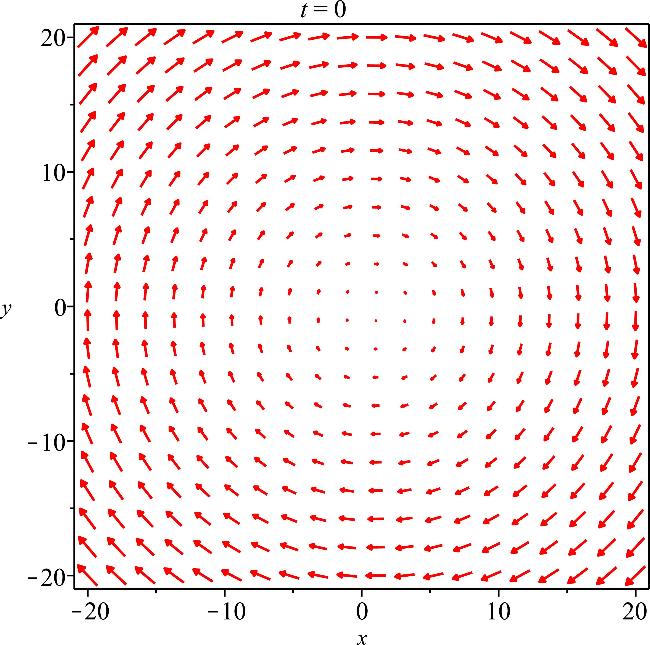
Interestingly, we find that the solution (3.10) takes a similar structure to what was given by An and Zhu in [13]. It is noticed that the solution obtained here is rotational unless a0 = 0 since rot u = −2a0 and meanwhile it has no additional Ermakov structure, which are two differences to the results in [13]. The structure of the solution (3.10) is depicted in figure 1. From this figure, we can clearly see that steady flow is rotational and the velocities of all particles of the fluid move from inwards to the origin, which is different to the behaviors of the radially symmetric solution given by Yuen et al in [12, 29].
Figure 1. The vortex structure of the solution ${\boldsymbol{u}}={({u}_{1},{u}_{2})}^{{\rm{T}}}$ given by (3.10). Here the parameters are selected as a0 = b0 = c0 = 1. The strength of the velocity field is expressed by the length of the arrow.
For the 3D compressible Navier–Stokes equation with k1 = 0, let A and J be the antisymmetric matrices of this form:
It is of interest to notice that the solution (3.11) to the Navier–Stokes equation takes the same form as that given by Fan and Yuen in [19] for the Euler equation, In fact, if we require the parameter k2 to be zero and g0 = −a0, then the equation (2.3) becomes the Euler equation and the solution (3.11) is just the solution for the Euler equation in [19].
4. The second reduction: time-dependent matrix A
Observation on the form of the matrix B and C in (2.6)–(2.7) motives us to decompose A into A = f(t)I when J = 0, which can lead to the explicit irrotational solutions for the Navier–Stokes equation (2.3). We would like to point out that different to the above section, here no restrictions are imposed. The main result is described in the following theorem.
Suppose that the matrix A can be decomposed into the form of
which shows that C is a symmetric matrix. When inserting the expressions of A and C into (2.9), we can obtain (4.2). Meanwhile, one can easily validate that the original solution (2.10) and (2.11) is reducible to (4.3) and (4.4) wherein b(t) and c(t) satisfy (4.5)–(4.7). The proof is completed. □
It is noticed that the intrusion of the function f makes the solution of equation (4.2) difficultly accessible. In the sequel, we restrict to the solvable case, in which the parameters are required to satisfy the following condition:
It is of interest to find that the above condition is compatible with the condition given in (1.3). And under this condition, equation (4.2) is readily reducible to:
where α is a constant of integration. It is noticed that the solution has no constraint on the numbers N and γ, which is an extension result given in [17].
Case 2: If ft + f2 ≠ 0, then we reformulate (4.11) into this form:
which shows that the solution f(t) for the NS equation (1.1) is dependent on the gas parameter γ and dimensional parameter N. Therefore, the following two cases needs to be considered:
(i). When the parameters γ and N satisfy $\gamma =1-\frac{2}{N}$, then the system (4.13) reduces to
where α and β are constants. This solution is bounded and its form is different from (4.12). It is worth pointing out that the solution (4.15) is analogues to what was given by Chow et al for the damped compressible Euler equation [18]. Indeed, when setting the Lamé viscosity coefficients h(ρ) and g(ρ) in (2.1) to be zero, it is just the solution derived by Chow and his co-authors in [18]. Here, the intrusion of the viscosity coefficients h(ρ) and g(ρ) renders it to constitute a general solution of the NS equation.
(ii). When the parameters γ and N satisfy $\gamma \ne 1-\frac{2}{N}$, the form of (4.13) suggests us to introduce an auxiliary function h via:
Interestingly, we find that the solution (4.19) not only takes a similar form to what was obtained by An et al for the compressible Euler equation [17] wherein no restrictions were imposed on the parameters γ and N, but also to what was given by An and Zhu for the compressible Navier–Stokes equation [13], wherein it admits the integrable Ermakov structure. Moreover, one can easily validate that when $\gamma =1-\frac{2}{N}$, the solution (4.19) becomes to (4.12) by taking c1 = 0 and c2 = 1. Thus, (4.19) is a more general solution of equation (4.11) in the case of $\gamma =1-\frac{2}{N}$.
To sum up, we have shown in the above that some explicit solutions of the NS equation (2.3) can be obtained via theorem 3 when requiring the parameters satisfying the condition (4.9). To shed light on this aspect, we shall give some illustrative examples.
For the 2D compressible NS equation, we take k1 + 2k2 = 0, $\gamma =\frac{1}{2}$, b(t) = 0, c(t) = 0 and
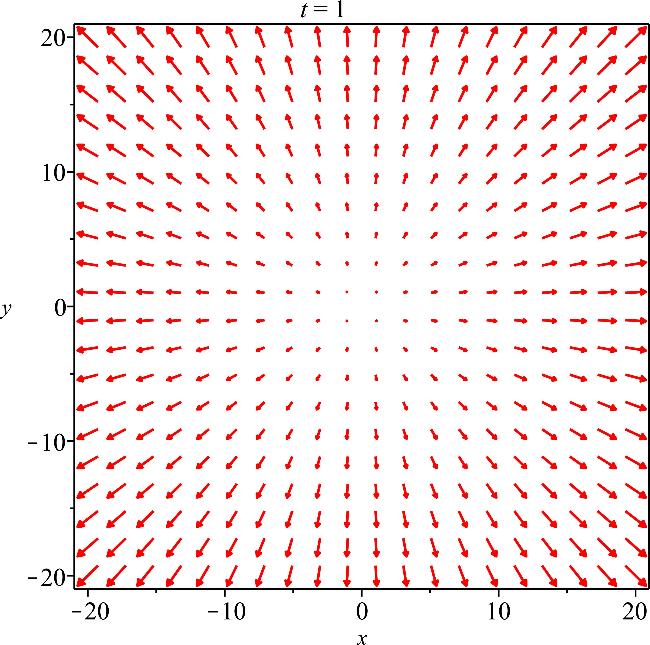
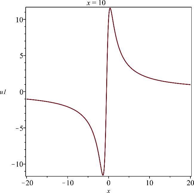
It is obvious that the solution (4.20) takes the similar structure to the solution given in [17]. Here, the solution has an irrotational structure, which can be seen in figure 2. When comparing it with the rotational solution given in (3.11), one can find that they are quite different to each other. In order to study the dynamical behaviors, we present the numerical figure in figure 3.
Figure 2. The irrotational structure of the velocity solution ${\boldsymbol{u}}={({u}_{1},{u}_{2})}^{{\rm{T}}}$ given by (4.20). Here the parameters are selected as c1 = c2 = c3 = 1. The strength of the velocity field is expressed by the length of the arrow.
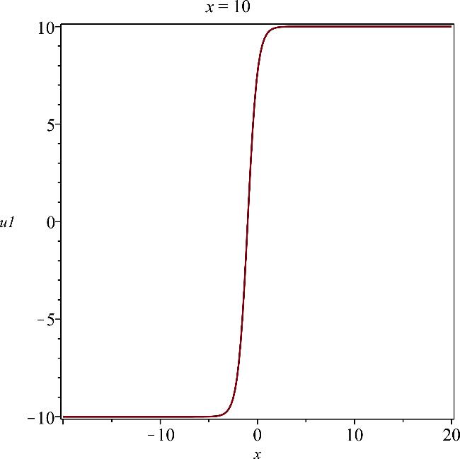
It is seen that the velocity of the fluid is bounded with respect to time, whose dynamical behavior is displayed in figure 4. Such a kind of bounded solution was previously obtained for the damped Euler equation in [18]. However, for the Navier–Stokes equation, it seems to be the first time to obtain this type of solution.
Figure 4. The bounded structure of the velocity solution u1 given by (4.21) at x1 = 10. Here the parameters are selected as α = 1 and β = 2.
5. The property of solutions to the NS equation
In this section, we shall investigate the structure and properties of solutions to the NS equation. For simplicity, we shall only consider the special case wherein k1 = 0, b(t) = 0 and c(t) = 0. Thus, under this case the solutions of the NS equations (2.10) and (2.11) can be written into the following form:
Here, we would like to show that there exists an almost linear superposition principle for the solutions (5.1) of the NS equation, which is established in the following theorem:
Assuming that A and C satisfy conditions of theorem 1, and u(x, t), u(y, t) are two arbitrary solutions in the form of (5.1). Then
In theorem 1, if A = J is an antisymmetric matrix, then for any constant γ ≥ 1, then the matrix −C = − A2 is positive definite, and the density function
The Navier–Stokes equation is an important physical model, which has been widely used in modelling fluids, plasmas, astrophysics, oceanography and atmospheric dynamics. In this paper, based on the matrix and curve integration techniques, we have built a sufficient condition for the existence of Cartesian vector solutions for the N-dimensional NS equation with Coriolis force and density-dependent viscosity. Among these solutions, some constitute the generalization of the results previously obtained by other authors and the bounded solution obtained in section 4 seems to be new. Based on the importance and applications of the NS equation, the results obtained here may provide a new perspective for expert to understand how the real fluid will flow. And they also provide benchmarks for testing and improving some numerical codes for computing more complicated flows.
However, there still remain many challenging problems that deserve deep considerations:
1). It is seen that the key to find solutions for the NS equation (2.3) is to solve the matrix differential equation (2.9), which contains N2 scalar equations. Due to its complexity, here we only handle two special solvable cases. Therefore, it is worth considering whether some other special cases that can lead to solutions for the NS equation exist.
2). It is noticed that the velocity function in the Cartesian vector solutions obtained here takes a linear function form of the spatial coordinates. Therefore, it is natural to inquire whether the solutions expressed by quadratic, cubic, or other nonlinear functions of the Cartesian coordinates exist in the NS equation (2.3). If they do exist, how to find the corresponding pressure function seems to be an intriguing research.
3). We know that in geophysical flows, there are many physical models which are closely linked to the NS equation, such as the Euler-Poisson and Navier–Stokes-Poisson equations. Therefore, it would be of interest to study whether the method can be applied to derive Cartesian vector solutions of these models.
We would like to express our sincere thanks to the reviewers for their helpful comments and valuable suggestions. This work is supported by the National Natural Science Foundation of China under grant Nos. 12371250, 42375002, Jiangsu Provincial Natural Science Foundation under grant No. BK20221508 and No. 2024-JSS-GF-095-06, by Hong Kong General Research Fund (GRF) under grant No. 18300821, 18300622 and 18300424.
RozanovaO S, TurzynskyM K2019 The stability of vortices in gas on the l-plane: the influence of centrifugal force Nonlinear Analysis and Boundary Value Problems101 131 143
3
GionaM, ProcopioG, AdroverA, MauriR2023 New formulation of the Navier–Stokes equations for liquid flows J. Non-equil. Thermody.48 207
BreschD, DesjardinsB2003 Existence of global weak solutions for a 2D viscous shallow water equations and convergence to the quasi-geostrophic model Comm. Math. Phys.238 211
MenonS H, RaoR A, MathewJ, JayaprakashJ2021 Derivation of Navier–Stokes equation in rotational frame for engineering flow analysis Int. J. Thermofluids11 100096
CodinaR1999 Numerical solution of the incompressible Navier–Stokes equations with Coriolis forces based on the discretization of the total time derivative J. Comput. Phys.148 467
AnH L, ZhuH X2022 The elliptical vortices, integrable Ermakov structure, Schrödinger connection, and Lax pair in the compressible Navier–Stokes equation Stud. Appl. Math.149 879
GuoZ H, XinZ P2012 Analytical solutions to the compressible Navier–Stokes equations with density-dependent viscosity coefficients and free boundaries J. Diff. Equ.253 1
AnH L, YuenM W2014 Drifting solutions with elliptic symmetry for the compressible Navier–Stokes equations with density-dependent viscosity J. Math. Phys.55 053506
FanE G, YuenM W2021 A method for constructing special solutions for multidimensional generalization of Euler equations with Coriolis force Chinese J. Phys.72 136
DrazinP G, RileyN2006The Navier–Stokes Equations: A Classification of Flows and Exact Solutions (London Mathematical Society Lecture Note Series) (Book 334) Cambridge University Press
28
CraikA D, CriminaleW O1986 Evolution of wavelike disturbances in shearows: a class of exact solutions of the Navier-Stokes equations Proc. R Soc. Lond A406 13


