


1. Introduction
In recent years, deep learning methods have emerged as a powerful alternative to traditional numerical approaches for solving both forward and inverse problems of partial differential equations (PDEs) and have been widely applied across various scientific and engineering domains [1–7]. Currently, various deep learning methods have been proposed and successfully applied to the study of PDEs. Representative approaches include the physics-informed neural networks (PINNs) [3], the deep operator networks [6], the deep Galerkin method [1], the local extreme learning machine [5], and the random feature method [7], among others. Among them, PINNs approximate the solutions of PDEs by training neural networks to minimize a composite loss function that integrates physical laws, initial/boundary conditions, and experimental or simulated data. Subsequently, researchers from various fields have introduced a series of improvements and extensions to the vanilla PINN formulation, all of which were aimed at enhancing its accuracy and robustness in order to tackle increasingly challenging problems arising in studying various PDEs, such as those with highly nonlinear, multi-scale, chaos or turbulence behavior [8–14]. Therefore, benefiting from the flexibility of physical laws and the diversity of data sources, PINNs and their various variants have been widely applied to solving various PDE models and addressing practical problems in science and engineering.
Rogue waves (also known as freak waves, extreme waves, giant waves or killer waves) are extremely rare, transient, and isolated large-amplitude waves whose most distinctive characteristic is a crest height at least twice that of the surrounding waves [15]. In 1965, Draper first proposed the concept of the rogue wave, which he named ‘Freak Ocean Wave' [16]. However, the existence of rogue waves lacked direct observational evidence for a long time, until January 1, 1995, when the Draupner oil platform recorded the first complete observation of a rogue wave, marking an important milestone in rogue wave research, and this wave is therefore also known as the ‘New Year Wave' [17]. To gain a deeper understanding of the formation mechanisms and dynamic characteristics of rogue waves, extensive theoretical analyses and experimental studies have been conducted across various disciplines. For decades, rogue wave theory has demonstrated significant research value in fields such as fluid dynamics [18], multistable system [19], nonlinear optics [20], Bose–Einstein condensates [21], plasma physics [22], and microwave transmission [23]. Additionally, rogue wave theory has gained widespread attention in financial markets, where researchers use mathematical models of financial rogue waves to explain extreme events such as stock market crashes, sharp exchange rate fluctuations, and systemic financial crises, revealing their intrinsic connection to nonlinear fluctuation mechanisms and providing theoretical support for understanding and predicting financial risks [24–27].
For decades, various option pricing models have been developed to more accurately describe the complex and dynamic features of financial markets and provide reasonable mathematical explanations, aiming to characterize the dynamics of financial assets and the market pricing mechanisms. In 1973, Black and Scholes pointed out that, under a series of idealized assumptions associated with a complete liquid market (i.e. the absence of transaction costs, taxes, and arbitrage opportunities, together with the assumption that stock prices follow a geometric Brownian motion), once options are correctly priced, profits could be made by creating a portfolio of long and short positions in both the options and the underlying asset, and they derived the theoretical valuation formula for options, known as the famous linear Black–Scholes (BS) equation [28]:
$\begin{eqnarray*}\begin{array}{r}\frac{\partial V}{\partial t}+r\left(S\frac{\partial V}{\partial S}-V\right)+\frac{{\sigma }^{2}}{2}{S}^{2}\frac{{\partial }^{2}V}{\partial {S}^{2}}=0,\end{array}\end{eqnarray*}$
in which V = V(t, S) is the market value of option, S is the price of the underlying stock, t denotes time, the domain is defined as 0 ≤ S < ∞, 0 ≤ t ≤ T, T is the expiry date. The σ is the volatility of stock price, and r ≥ 0 is the risk-free interest rate. In this model, the underlying stock (asset) price S is assumed to follow a geometric Brownian motion with the volatility σ and drift μ, satisfying the stochastic differential equation dS(t) = μS(t)dt + σS(t)dW(t) [29], where W(t) is the standard Wiener process. The solution of the linear BS equation indicates that any derivative and any asset can be perfectly replicated or perfectly hedged by a portfolio of other assets available in the market (see [30]). The introduction of the BS model laid the foundation for modern financial engineering, with empirical evidence showing that its theoretical option prices closely matched market observations under ideal conditions, leading to widespread application in real trading and becoming a key cornerstone for subsequent derivative pricing theories [31].However, these assumptions of a complete liquid market often fail to hold in reality, as real markets are subject to factors such as transaction costs, insufficient liquidity, and volatility fluctuations. Consequently, in recent years, incomplete markets and markets characterized by limited liquidity (or illiquidity) have attracted increasing attention. Due to transaction costs, large investor preferences, and market incompleteness, classical BS models may give rise to strong or fully nonlinear dynamics behaviors, in which the volatility σ and drift μ can depend on the stock price S or the derivatives of the option price V itself. Therefore, as noted in [32–34], the most general equation governing European option prices is the following nonlinear BS equation: 1.1 ) with r = 0 has also been investigated in [32–34, 36]. In [34], Patsiuk and Kovalenko employed symmetry reduction to investigate several exact solutions of the nonlinear BS transaction cost model, and applied these solutions to several boundary value problems.
$\begin{eqnarray*}\begin{array}{r}\frac{\partial V}{\partial t}+r\left(S\frac{\partial V}{\partial S}-V\right)+\frac{{\tilde{\sigma }}^{2}(S,{V}_{S},{V}_{SS})}{2}{S}^{2}\frac{{\partial }^{2}V}{\partial {S}^{2}}=0.\end{array}\end{eqnarray*}$
Here, $\tilde{\sigma }(S,{V}_{S},{V}_{SS})$ denotes the modified volatility function. In this work, we primarily focus on a transaction cost model with a wave function of the following form [35]: $\begin{eqnarray*}\begin{array}{r}{\tilde{\sigma }}^{2}(S,{V}_{S},{V}_{SS})={\sigma }^{2}\left(1+2\rho S\frac{{\partial }^{2}V}{\partial {S}^{2}}\right),\end{array}\end{eqnarray*}$
in which σ is the constant (historical) volatility, and ρ indicates a parameter modeling the liquidity of the market under study, we have σ, ρ > 0. Thus the nonlinear BS transaction cost model can be written as: $\begin{eqnarray}\frac{\partial V}{\partial t}+r\left(S\frac{\partial V}{\partial S}-V\right)+\frac{{\sigma }^{2}}{2}{S}^{2}\frac{{\partial }^{2}V}{\partial {S}^{2}}\left(1+2\rho S\frac{{\partial }^{2}V}{\partial {S}^{2}}\right)=0.\end{eqnarray}$
In particular, if ρ = 0, the market is complete liquid (and the above equation reduces to the linear BS equation), whereas for large ρ, trades exert a substantial impact on transaction prices. Therefore, in this work, ρ is generally assumed to be small. If r = 0, it implies that there is no risk-free return in the market, i.e. no time value of money. In financial terms, this corresponds to a zero interest rate environment, where the discount factor equals 1 and future cash flows do not need to be discounted. The above equation (The linear BS equation can be solved analytically to compute the prices of European options, and is applicable to both call and put options. A European call option is a contract that grants its holder the right to purchase a specified asset (referred to as the underlying asset S(t)) at a predetermined price (known as the strike or exercise price K) on a specified future date (called the expiry date T). If the holder chooses to exercise the right, the counterparty or seller is obliged to deliver the asset. Accordingly, the value of the option at maturity, known as the payoff function, is given by V(T, S) = (S − K)+. Conversely, a European put option grants the right to sell the underlying asset, with the payoff function given by V(T, S) = (K − S)+ [37]. The nonlinear BS model typically accounts for more complex market factors than the traditional linear BS model, such as transaction costs, market liquidity, and volatility variations. These models may more realistically reflect market conditions by incorporating nonlinear terms or stochastic elements, thereby facilitating the pricing of European options. Nonlinear BS models generally require numerical methods for their solution, as their equations are more complex and highly sensitive to changes in parameters and independent variables, making analytical solutions difficult to obtain [38]. Therefore, in this study, we aim to employ advanced deep learning methods to numerically predict the evolution and nonlinear dynamics of European option prices under a nonlinear BS transaction cost model in illiquid and incomplete markets.
Moreover, the assumption of constant volatility in classical stochastic differential equations fails to capture the volatility skew observed in real markets and cannot adequately explain the sharp fluctuations in option prices during economic crises [39]. Especially after the 1997 Asian financial crisis, it became increasingly evident that traditional stochastic models could not fully capture the complex dynamics of financial markets, leading to the development of various improved mathematical models aimed at providing a more accurate representation of the highly dynamic and evolving nature of financial markets [40, 41]. In 1997, Baaquie proposed a novel way to option pricing by applying path integral methods from quantum mechanics, effectively constructing a connection between the price of a stock option and the Schrödinger wave function [42]. In 2004, Haven further proposed that if the option price is regarded as a state function, it satisfies a specific potential function of the Schrödinger equation, and pointed out that the solution of the BS equation can be mapped to the linear Schrödinger equation [43]. In 2009, in order to construct a pricing model that could more accurately capture the nonlinear complexity of the market, Ivancevic proposed a novel nonlinear option pricing model, known as the Ivancevic option pricing model [44], as follows: 1.2 ) can be chosen to be negative since the option price wave function φ is invariant under the translation transformation t → t + Ti. Then, four types of analytical solutions of the NLS equation are provided in terms of Jacobi elliptic functions, all starting from de Broglie's plane-wave packet associated with the free quantum-mechanical particle [44]. The validity of the solution was verified through unsupervised Hebbian learning or the supervised Levenberg–Marquardt algorithm, and it was demonstrated that the solution is consistent with the BS model under certain conditions [44]. In 2010, Yan presented the concept of financial rogue waves based on the Ivancevic option pricing model and demonstrated that financial rogue waves can serve as a phenomenological description of extreme events in financial markets (such as financial crises/storms) and related fields [24]. Therefore, the Ivancevic option pricing model can describe potential extreme financial phenomena, where the option price φ depends on the stock price S, and S itself is a time-dependent stochastic variable, making it difficult to determine the actual data (including upper and lower boundary data) for stock and option prices over a future period. In this study, we are more interested in how to integrate the Ivancevic option pricing model with state of the art deep learning method to predict potential extreme financial phenomena (i.e. financial rogue waves) using only initial data at the current moment, thereby enhancing the capability of proactive analysis for market risk management and financial stability.
$\begin{eqnarray}\begin{array}{r}{\rm{i}}\frac{\partial \phi (t,S)}{\partial t}+\frac{1}{2}\sigma \frac{{\partial }^{2}\phi (t,S)}{\partial {S}^{2}}+\beta | \phi (t,S){| }^{2}\phi (t,S)=0,\end{array}\end{eqnarray}$
here φ = φ(t, S) represents the option price wave function, the dispersion frequency coefficient σ is the volatility (which itself can be either a constant or a stochastic process), and the Landau coefficient β represents the adaptive market potential, which is essentially a nonlinear Schrödinger (NLS) equation. Notice that time t in equation (Due to the ‘appearing and disappearing without a trace' feature of rogue waves, predicting financial rogue waves using deep learning methods driven solely by initial data is a highly challenging task. In other words, the predictability of financial rogue waves largely depends on the accuracy of the initial data and is extremely sensitive to small variations in initial conditions. This sensitivity is particularly pronounced in complex problems such as highly nonlinear, multi-scale, chaos or turbulence behavior, making it difficult for traditional methods to effectively model and predict. Moreover, the nonlinear BS transaction cost model is essentially a variable-coefficient PDE. Due to its strong nonlinearity, the multiscale nature of the risk-free rate r under small-parameter conditions, and its sensitivity to changes in the independent variables, conventional numerical methods often struggle to solve it efficiently. Recently, Wang et al pointed out that when dealing with complex tasks that are highly sensitive to initial data (such as highly nonlinear, multi-scale, chaos or turbulence behavior problems), the existing PINN formulation fails to respect the inherent spatiotemporal causal structure of the physical system's evolution, which may ultimately lead the PINN model to converge to incorrect solutions [13]. To address this issue, they proposed the respecting causality PINN (RCPINN) by constructing a reformulation of the PINN loss function that more explicitly reflects the physical causal relationships during the model's training. Multiple numerical experiments demonstrated that this simple yet crucial modification significantly improved the model's prediction accuracy. To the best of our knowledge, some existing studies have applied deep learning methods to solve the (1 + 1) dimensional focusing NLS equation for rogue waves [14, 45, 46], as well as financial rogue waves in the Ivancevic option pricing model and the pricing of European options under the linear BS equation [47], but these studies have all been based on Dirichlet boundary conditions. However, in real, complex, and dynamic financial markets, the upper and lower boundary data for future time periods cannot be obtained, making the setting of the Dirichlet boundary condition obviously inconsistent with the actual conditions of financial markets. Therefore, in this work, we for the first time employ the RCPINN to predict the evolution of financial rogue waves described by the Ivancevic option pricing model, as well as predicting the evolution and complex dynamics behaviors of European option prices under the nonlinear BS transaction cost model. The goal is to enhance the predictive capability for market extreme volatility events and the pricing of complex European options based solely on initial data, and to further explore the potential value of deep learning methods in financial risk management and option pricing theory.
The structure of this paper is as follows: section 2 provides a detailed introduction to the RCPINN and other enhanced techniques. Section 3 presents numerical results for predicting financial rogue waves and predicting the evolution of European option prices by employing the RCPINN only with initial data. Section 4 concludes the paper and discusses the future applications and developments of deep learning method in the financial market and financial derivatives.
2. Methodology
In this part, we take a detail overview of the RCPINN [13] in the context of solving nonlinear option pricing models. For convenience, we take the prediction of financial rogue waves in the Ivancevic option pricing model as an example to detail the principle and architecture of the RCPINN.
• Respecting causality physics-informed neural network
Specifically, we consider the Ivancevic option pricing model with corresponding initial and periodic boundary conditions take the form 2.1 ), thereby u(t, S), v(t, S) and ${{ \mathcal I }}_{u}(S),\,{{ \mathcal I }}_{v}(S)$ are real-valued function for neural network training. Subject to the initial conditions 2.1 ). Then, we represent the unknown solution φ(t, S) by a deep fully-connected neural network φθ(t, S) with $\tanh $ activation function, in which θ denotes all tunable parameters of the neural network (including weights and biases). Now, a neural network model can be trained by minimizing the following total loss function
$\begin{eqnarray}\begin{array}{rc} & {\rm{i}}\frac{\partial \phi (t,S)}{\partial t}+\frac{1}{2}\sigma \frac{{\partial }^{2}\phi (t,S)}{\partial {S}^{2}}+\beta | \phi (t,S){| }^{2}\phi (t,S)=0,\\ & t\in [{T}_{i},{T}_{f}],\quad S\in [{S}_{l},{S}_{r}],\phi ({T}_{i},S)={ \mathcal I }(S),S\in [{S}_{l},{S}_{r}],\\ & \phi (t,{S}_{l})=\phi (t,{S}_{r}),\,{\phi }_{S}(t,{S}_{l})={\phi }_{S}(t,{S}_{r}),t\in [{T}_{i},{T}_{f}],\end{array}\end{eqnarray}$
where Ti and Tf respectively indicate the initial time and final time, while Sl and Sr indicate the left and right boundaries of space. ${ \mathcal I }$ is initial operator. For the sake of simplicity in neural network training, we set $\phi (t,S)=u(t,S)\,+{\rm{i}}v(t,S),\,{ \mathcal I }(S)={{ \mathcal I }}_{u}(S)+{\rm{i}}{{ \mathcal I }}_{v}(S)$ in equation ( $\begin{eqnarray}\begin{array}{r}u({T}_{i},S)={{ \mathcal I }}_{u}(S),v({T}_{i},S)={{ \mathcal I }}_{v}(S),S\in [{S}_{l},{S}_{r}],\end{array}\end{eqnarray}$
and periodic boundary conditions $\begin{eqnarray}\begin{array}{l}u(t,{S}_{l})=u(t,{S}_{r}),\,v(t,{S}_{l})=v(t,{S}_{r}),\\ {u}_{S}(t,{S}_{l})={u}_{S}(t,{S}_{r}),\,{v}_{S}(t,{S}_{l})={v}_{S}(t,{S}_{r}),\\ t\in [{T}_{i},{T}_{f}],\end{array}\end{eqnarray}$
where φ describes the unknown latent solution which is governed by the Ivancevic option pricing model ( $\begin{eqnarray}\begin{array}{r}{ \mathcal L }({\boldsymbol{\theta }})={\lambda }_{ic}{{ \mathcal L }}_{ic}({\boldsymbol{\theta }})+{\lambda }_{bc}{{ \mathcal L }}_{bc}({\boldsymbol{\theta }})+{\lambda }_{r}{{ \mathcal L }}_{r}({\boldsymbol{\theta }}).\end{array}\end{eqnarray}$
Since we are considering the periodic boundary conditions (2.3 ) of the Ivancevic option pricing model (2.1 ), in order to further simplify the training objective (2.4 ), we rigorously enforce the periodic boundary conditions by embedding the input coordinates into Fourier expansion utilizing equation (2.12 ), with non-negative integer m. Then the total loss function (2.4 ) can be reduced to 2.7 ) can be rewritten as
$\begin{eqnarray}\begin{array}{r}{ \mathcal L }({\boldsymbol{\theta }})={\lambda }_{ic}{{ \mathcal L }}_{ic}({\boldsymbol{\theta }})+{\lambda }_{r}{{ \mathcal L }}_{r}({\boldsymbol{\theta }}),\end{array}\end{eqnarray}$
where hyper-parameters {λic, λr} provide the flexibility to assign distinct learning rates to each loss term, enabling a balanced interaction among them throughout the model training process. The initial condition loss ${{ \mathcal L }}_{ic}({\boldsymbol{\theta }})$ can be defined as $\begin{eqnarray}\begin{array}{rcl}{{ \mathcal L }}_{ic}({\boldsymbol{\theta }}) & = & \frac{1}{{N}_{ic}}\displaystyle \sum _{i=1}^{{N}_{ic}}| u({T}_{i},{S}_{ic}^{i})-{{ \mathcal I }}_{u}({S}_{ic}^{i}){| }^{2}\\ & & +\frac{1}{{N}_{ic}}\displaystyle \sum _{i=1}^{{N}_{ic}}| v({T}_{i},{S}_{ic}^{i})-{{ \mathcal I }}_{v}({S}_{ic}^{i}){| }^{2}.\end{array}\end{eqnarray}$
For respecting causality for training RCPINN, we suppose ${\{{t}_{i}\}}_{i=1}^{{N}_{t}}$ uniformly discretize the temporal domain [Ti, Tf] (here ${T}_{i}={t}_{1}\lt {t}_{2}\lt \cdots \lt {t}_{{N}_{t}}={T}_{f}$), and ${\{{S}_{j}\}}_{j=1}^{{N}_{x}}$ uniformly discretize the spatial domian [Sl, Sr]. Then the weighted residual loss ${{ \mathcal L }}_{r}({\boldsymbol{\theta }})$ can be defined as $\begin{eqnarray}\begin{array}{r}{{ \mathcal L }}_{r}({\boldsymbol{\theta }})=\frac{1}{{N}_{t}}\displaystyle \sum _{i=1}^{{N}_{t}}{w}_{i}{{ \mathcal L }}_{r}({t}_{i},{\boldsymbol{\theta }}),\end{array}\end{eqnarray}$
in which wi should be large, thus allow the minimization of ${{ \mathcal L }}_{r}({t}_{i},{\boldsymbol{\theta }})$ only if all residuals ${\{{{ \mathcal L }}_{r}({t}_{k},{\boldsymbol{\theta }})\}}_{s=1}^{i-1}$ before ti are minimized properly, and vice versa. the weights wi can be represented as $\begin{eqnarray}\begin{array}{r}{w}_{i}=\exp \left[-\epsilon \displaystyle \sum _{l=1}^{i-1}{{ \mathcal L }}_{r}({t}_{l},{\boldsymbol{\theta }})\right],\,{\rm{for}}\,i=2,3,\cdots ,\,{N}_{t},\end{array}\end{eqnarray}$
where ε is the causality parameter that controls the steepness of the weights wi. Then, the residual loss ${{ \mathcal L }}_{r}({t}_{i},{\boldsymbol{\theta }})$ in equation ( $\begin{eqnarray}\begin{array}{rcl}{{ \mathcal L }}_{r}({t}_{i},{\boldsymbol{\theta }}) & = & \frac{1}{{N}_{S}}\displaystyle \sum _{j=1}^{{N}_{S}}\left|-\frac{\partial v}{\partial t}({t}_{i},{S}_{j})+\frac{1}{2}\sigma \frac{{\partial }^{2}u}{\partial {S}^{2}}({t}_{i},{S}_{j})\right.\\ & & +{\left.\beta u({t}_{i},{S}_{j})[u{({t}_{i},{S}_{j})}^{2}+v{({t}_{i},{S}_{j})}^{2}]\Space{0ex}{3.25ex}{0ex}\right|}^{2}\\ & & +\left.\frac{1}{{N}_{S}}\displaystyle \sum _{j=1}^{{N}_{S}}\right|\frac{\partial u}{\partial t}({t}_{i},{S}_{j})\\ & & +{\left.\frac{1}{2}\sigma \frac{{\partial }^{2}v}{\partial {S}^{2}}({t}_{i},{S}_{j})+\beta v({t}_{i},{S}_{j})[u{({t}_{i},{S}_{j})}^{2}+v{({t}_{i},{S}_{j})}^{2}]\right|}^{2}.\end{array}\end{eqnarray}$
Clearly, the weights wi exhibits an exponential inverse relationship with the magnitude of the accumulative residual loss from the previous time steps. As a result, ${{ \mathcal L }}_{r}({t}_{i},{\boldsymbol{\theta }})$ cannot be minimized unless all previous residuals ${\{{{ \mathcal L }}_{r}({t}_{l},{\boldsymbol{\theta }})\}}_{l=1}^{i-1}$ are reduced to a sufficiently small value, ensuring that wi becomes large enough. This straightforward yet highly effective strategy ensures that RCPINN explicitly respects physical causality during the training phase, making it particularly well-suited for predicting financial rogue waves, which heavily rely on initial data.
The choice of the causality parameter ε. We must emphasize that the results generated by the proposed weighted residual loss ${{ \mathcal L }}_{r}({\boldsymbol{\theta }})$ are notably sensitive to variations in the causality parameter ε. One can observe that opting for a larger ε value might result in a more difficult optimization process, since the residuals at earlier times need to be minimized to extremely small values to trigger the latter temporal weights. Conversely, choosing a very small ε can impede the network's capacity to adequately minimize the residuals at subsequent times. Thereby, in order to choose an appropriate causality parameter ε and avoid laborious hyper-parameter tuning, we employ an annealing strategy by utilizing an incrementally increasing sequence of values ${\{{\epsilon }_{i}\}}_{s=1}^{p}$ that progressively strengthen the enforcement of the PDE residual constraints.
A stopping criterion for assessing training convergence. By monitoring the magnitude of the residual weights {wi}, one can establish an effective stopping criterion to evaluate the convergence of the RCPINN model throughout the training process. Specifically, one can choose to stop training when $\mathop{\min }\limits_{i}{w}_{i}\gt \delta $, where δ ∈ (0, 1) is a selected threshold parameter.
• Additional enhancement technologies
In this part, we employ a few important extensions and necessary settings that can further enhance RCPINN's performance in terms of accuracy and computational efficiency.
Modified multi-layer perceptrons. From [48], Wang et al presented a novel neural network architecture by introducing two transformer networks that project the inputs variables to a high-dimensional feature space and utilizing a pointwise multiplication operation to update the hidden layers, whose forward propagation rule as
$\begin{eqnarray}\begin{array}{rcl}{\boldsymbol{U}} & = & \sigma ({\boldsymbol{X}}{{\boldsymbol{W}}}^{1}+{{\boldsymbol{b}}}^{1}),\\ {\boldsymbol{V}} & = & \sigma ({\boldsymbol{X}}{{\boldsymbol{W}}}^{2}+{{\boldsymbol{b}}}^{2}),\\ {{\boldsymbol{H}}}^{(1)} & = & \sigma ({\boldsymbol{X}}{{\boldsymbol{W}}}^{(1)}+{{\boldsymbol{b}}}^{(1)}),\\ {{\boldsymbol{Z}}}^{(k)} & = & \sigma ({{\boldsymbol{H}}}^{(k)}{{\boldsymbol{W}}}^{(k+1)}+{{\boldsymbol{b}}}^{(k+1)}),\\ k & = & 1,\cdots ,\,L-1,\\ {{\boldsymbol{H}}}^{(k+1)} & = & (1-{{\boldsymbol{Z}}}^{(k)})\odot {\boldsymbol{U}}+{{\boldsymbol{Z}}}^{(k)}\odot {\boldsymbol{V}},\\ {{\boldsymbol{F}}}_{{\boldsymbol{\theta }}}({\boldsymbol{X}}) & = & {{\boldsymbol{H}}}^{(L)}{{\boldsymbol{W}}}^{L+1}+{{\boldsymbol{b}}}^{L+1},\end{array}\end{eqnarray}$
where X indicates an batch of the input data points, σ represents nonlinear activation function, and ⊙ denotes a point-wise multiplication. Here we refer to this novel architecture as modified multi-layer perceptrons. All trainable parameters can be written as $\begin{eqnarray}\begin{array}{r}{\boldsymbol{\theta }}=\{{{\boldsymbol{W}}}^{1},{{\boldsymbol{b}}}^{1},{{\boldsymbol{W}}}^{2},{{\boldsymbol{b}}}^{2},{[{{\boldsymbol{W}}}^{(k)},{{\boldsymbol{b}}}^{(k)}]}_{k=1}^{L+1}\}.\end{array}\end{eqnarray}$
The modified multi-layer perceptrons architecture demonstrates greater effectiveness compared to standard multi-layer perceptrons in minimizing PDE residuals and accurately capturing sharp gradients.Exact imposition of periodic boundary conditions. It is widely known that the inexact imposition of boundary conditions may harm the neural network's performance and training stability. For accurately imposing periodic boundary conditions, Dong et al proposed that periodic boundary conditions can be strictly enforced as hard constraints by constructing Fourier feature embedding of the input data [49]. Specifically, if we consider a smooth function f(t, S) with periodic P (namely f(t, S) = f(t, S + P)), the periodic constraint of f(t, S) can be encoded in a neural network by means of a one-dimensional Fourier feature embedding
$\begin{eqnarray}{f}^{{\prime} }(t,S)=[t,1,\cos (\omega S),\sin (\omega S),\ldots ,\,\cos (m\omega S),\sin (m\omega S)],\end{eqnarray}$
where $\omega =\frac{2\pi }{P}$, and non-negative integer m can be set arbitrarily. Thereby, for any network output Fθ, it can be proved that any ${{\boldsymbol{F}}}_{{\boldsymbol{\theta }}}({f}^{{\prime} }(t,S))$ exactly satisfies the periodic constraint.Figure 1 displays schematic architecture of the RCPINN for predicting financial rogue waves of Ivancevic option pricing model. Figure 1 comprises four key components: (I). The network input with Fourier feature embedding is processed through a modified multi-layer perceptrons containing two transformation networks to generate outputs, where the Fourier embedding ensures exact imposition of periodic boundary conditions. (II). The Ivancevic option pricing model and its initial conditions (providing initial training points) are incorporated as physics-informed constraints, which connect to the network outputs from Part (I) via automatic differentiation. (III). The loss function ${ \mathcal L }$ structure explicitly illustrates the causal parameters ε, weights wi of residual loss, initial condition loss ${{ \mathcal L }}_{ic}$ and residual loss ${{ \mathcal L }}_{r}$. (IV). The spatiotemporal domain [Ti, Tf] × [Sl, Sr] is uniformly divided (collocation points sampled via uniform grids), and Adam optimizer is utilized for network training, while a reconstructed residual loss function ${ \mathcal L }$ in Part (III) base on uniformly segmented time regions enforcing network respect the temporal causal structure during training.
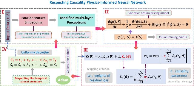
Figure 1. Schematic architecture of the RCPINN for predicting financial rogue waves of Ivancevic option pricing model. |
3. Numerical results
In this part, we employ the RCPINN to predict financial rogue waves of Ivancevic option pricing model and providing the price of European option in nonlinear BS transaction-cost model. Here, we first present the corresponding hyper-parameters settings in this work. We set λic = 100, λr = 1, Nt = 50, NS = 64. The incrementally increasing causality parameter sequence ${\{{\epsilon }_{i}\}}_{s=1}^{5}=[1{0}^{-3},1{0}^{-2},1{0}^{-1},1{0}^{0},1{0}^{1}]$, the threshold of stopping criterion δ = 0.99. The network architecture of RCPINN is configured as [2, 40, 40, 40, 2/1]. All networks are trained via stochastic gradient descent utilizing the Adam optimizer with default settings [50] and an exponential learning rate decay with a decay-rate of 0.9 per 5000 training iterations. All numerical experiments are done with 13th Gen Inter(R) Core(TM) i9-13900HX CPU processor and NVIDIA GeForce RTX 4060 GPU processor on the Windows 11 operating system.
3.1. Financial rogue waves of Ivancevic option pricing model
In this part, we numerically predict the first-order and second-order financial rogue waves of the Ivancevic option pricing model by utilizing the RCPINN only with initial data.
• First-order financial rogue wave
From [24], The first-order financial rogue wave of equation (1.2 ) for the option-price wave function φ(t, S) is expressed through complex rational functions of the stock price S and time t in the form 3.1 ) to 3.3 ), and select Nc = NtNS collocation points for each causality parameter. Now, we employ the RCPINN to predict the first-order financial rogue wave. Then, by means of the Adam optimizer with a maximum of 20 000 iterations, the relative L2 norm error of the RCPINN model achieves 1.641e-02 for the predicted first-order financial rogue wave φ(t, S) in 394.2784 s.
$\begin{eqnarray}\begin{array}{rcl}{\phi }_{1}(t,S) & = & \alpha \sqrt{\frac{\sigma }{2\beta }}\left[1-\frac{4(1+{\rm{i}}\sigma {\alpha }^{2}t)}{1+2{\alpha }^{2}{(S-\sigma kt)}^{2}+{\sigma }^{2}{\alpha }^{4}{t}^{2}}\right]\\ & & \times {{\rm{e}}}^{{\rm{i}}\left[kS+\frac{1}{2}\sigma ({\alpha }^{2}-{k}^{2})t\right]},\end{array}\end{eqnarray}$
in which σβ > 0. Especially, once we choose $\sigma =2,\beta =\frac{1}{4},\alpha =1,k=0$, one can reduce the equation ( $\begin{eqnarray}\begin{array}{r}{\phi }_{1}(t,S)=\left(\frac{-16{\rm{i}}t+4{S}^{2}+8{t}^{2}-6}{1+2{S}^{2}+4{t}^{2}}\right){{\rm{e}}}^{{\rm{i}}t}.\end{array}\end{eqnarray}$
Then, we consider the following initial condition within domain [−5, 5] × [−1, 1] $\begin{eqnarray}{ \mathcal I }(S)={\phi }_{1}(-1,S),\quad S\in [-5,5].\end{eqnarray}$
Next, we obtain Nic = 512 initial training points by means of initial condition (Figure 2 manifests the deep learning results of the predicted first-order financial rogue wave φ(t, S) stemming from the RCPINN for Ivancevic option pricing model (1.2 ). Figure 2(a) displays the density plots of the truth dynamics, prediction dynamics and error dynamics, and provides its corresponding amplitude scale size on the right side of error dynamics, as well as exhibits the sectional drawings which contain the true and predicted first-order financial rogue wave at five different moments. The three-dimensional plot with contour map for the predicted first-order financial rogue wave is displayed in figure 2(b). As evidenced in figures 2(a) and (b), the RCPINN framework demonstrates its capability to successfully predict the emergence of financial rogue waves, which is characterized by localized amplitude maxima in the option pricing wave function φ(t, S) at specific future time t and stock prices S, while utilizing only few initial training data. This data-efficient prediction of extreme wave phenomena may offer valuable insights for modeling and anticipating anomalous events in financial markets and related domains. Due to our adoption of an annealing strategy for selecting the causality parameter ε, figure 2(c) presents the evolution curves of the total loss function ${ \mathcal L }$, initial condition loss function ${{ \mathcal L }}_{ic}$, and weighted residual loss function ${{ \mathcal L }}_{r}$ during model training under five progressively increasing causality parameters [10−3, 10−2, 10−1, 100, 101]. Similarly, figure 2(d) showcases the evolution curves of minimum weights ${{\rm{\min }}}_{i}\,{w}_{i}$ during network training under five incrementally increasing causality parameters. Notably, the Adam optimizer terminated early (before reaching 20 000 iterations) for ε = 10−3, 10−2, 10−1 as the minimal residual weights ${{\rm{\min }}}_{i}{w}_{i}\gt 0.99$ met our stopping criterion, explaining why the loss curves in figure 2(c) are truncated for these cases. To better illustrate the evolution of the three loss functions and minimal residual weights ${{\rm{\min }}}_{i}\,{w}_{i}$ under the annealing strategy and stopping criterion, we provide comprehensive training results in table 1.
Figure 2. The training results of the first-order financial rogue wave φ(t, S) for the Ivancevic option pricing model arising from the RCPINN. (a) The ground truth, prediction and error dynamics density plots, as well as sectional drawings which contain the true and predicted first-order financial rogue wave at five distinct moments; (b) the three-dimensional plot with contour map for the predicted first-order financial rogue wave; (c) the evolution curve figures of three loss functions with different causality parameters during network training; (d) the evolution curve graph of minimal residual weights ${{\rm{\min }}}_{i}\,{w}_{i}$ during network training. |
Table 1. The comprehensive training results for predicting the first-order financial rogue wave. |
| ε | Adam | ${ \mathcal L }$ | ${{ \mathcal L }}_{ic}$ | ${{ \mathcal L }}_{r}$ | ${{\rm{\min }}}_{i}\,{w}_{i}$ |
|---|---|---|---|---|---|
| 10−3 | 3200 | 1.3894e-01 | 1.0181e-04 | 1.2919e-01 | 0.9937 |
| 10−2 | 7700 | 2.0406e-02 | 4.5042e-05 | 1.5841e-02 | 0.9923 |
| 10−1 | 15 500 | 2.2967e-03 | 2.9919e-06 | 1.9778e-03 | 0.9908 |
| 100 | 20 000 | 2.3383e-03 | 6.1185e-06 | 1.7011e-03 | 0.9209 |
| 101 | 20 000 | 5.9650e-04 | 2.1499e-06 | 3.8017e-04 | 0.8414 |
• Second-order financial rogue wave
Moreover, based on [24], the second-order financial rogue wave of equation (1.2 ) can be written as 3.4 ) can be reduced to: 1.2 ) in domain [−5, 5] × [−1, 1] as bellow 3.6 ), we choose Nic = 512 initial training points, as well as Nc = NtNS collocation points in the RCPINN. By applying the Adam optimizer with a maximum of 50 000 iterations, then the relative L2 norm error reaches 3.881e-02 for predicted second-order financial rogue wave φ(t, S) in 1152.7652 s.
$\begin{eqnarray}\begin{array}{rcl}{\phi }_{2}(t,S) & = & \alpha \sqrt{\frac{\sigma }{2\beta }}\left[1+\frac{A(t,S)+{\rm{i}}B(t,S)}{C(t,S)}\right]\\ & & \times {{\rm{e}}}^{{\rm{i}}[kS+\frac{1}{2}\sigma ({\alpha }^{2}-{k}^{2})t]},\end{array}\end{eqnarray}$
where σβ > 0, and the functions U(t, S), V(t, S), and W(t, S) adopt polynomial representations with respect to the stock price S and time t, with their explicit forms given below: $\begin{eqnarray*}\begin{array}{rcl}A(t,S) & = & \frac{3}{8}-\frac{1}{2}{\alpha }^{4}{(S-\sigma kt)}^{4}-\frac{3}{2}{\alpha }^{6}{\sigma }^{2}{t}^{2}{(S-\sigma kt)}^{2}\\ & & -\frac{5}{8}{\alpha }^{8}{\sigma }^{4}{t}^{4}-\frac{3}{2}{\alpha }^{2}{(S-\sigma kt)}^{2}-\frac{9}{4}{\alpha }^{4}{\sigma }^{2}{t}^{2},\\ B(t,S) & = & -\frac{1}{2}{\alpha }^{2}\sigma t\left[\Space{0ex}{3.00ex}{0ex}{\alpha }^{4}{(S-\sigma kt)}^{4}\right.\\ & & +{\alpha }^{6}{\sigma }^{2}{t}^{2}{(S-\sigma kt)}^{2}+\frac{1}{4}{\alpha }^{8}{\sigma }^{4}{t}^{4}\\ & & \left.-3{\alpha }^{2}{(S-\sigma kt)}^{2}+\frac{1}{2}{\alpha }^{4}{\sigma }^{2}{t}^{2}-\frac{15}{4}\right],\\ C(t,S) & = & \frac{3}{32}+\frac{1}{12}{\alpha }^{6}{(S-\sigma kt)}^{6}\\ & & +\frac{1}{8}{\alpha }^{8}{\sigma }^{2}{t}^{2}{(S-\sigma kt)}^{4}+\frac{1}{16}{\alpha }^{10}{\sigma }^{4}{t}^{4}{(S-\sigma kt)}^{2}\\ & & +\frac{1}{96}{\alpha }^{12}{\sigma }^{6}{t}^{6}\\ & & +\frac{1}{8}{\alpha }^{4}{(S-\sigma kt)}^{4}-\frac{3}{8}{\alpha }^{6}{\sigma }^{2}{t}^{2}{(S-\sigma kt)}^{2}\\ & & +\frac{9}{32}{\alpha }^{8}{\sigma }^{4}{t}^{4}+\frac{9}{16}{\alpha }^{2}{(S-\sigma kt)}^{2}\\ & & +\frac{33}{32}{\alpha }^{4}{\sigma }^{2}{t}^{2}.\end{array}\end{eqnarray*}$
Particularly, as we set $\sigma =2,\beta =\frac{1}{4},\alpha =1,k=0$, the above equation ( $\begin{eqnarray}{\phi }_{2}(t,S)=\frac{D(t,S)}{8{S}^{6}+(48{t}^{2}+12){S}^{4}+96{\left({t}^{2}-\frac{3}{4}\right)}^{2}{S}^{2}+64{t}^{6}+432{t}^{4}+396{t}^{2}+9}{{\rm{e}}}^{{\rm{i}}t},\end{eqnarray}$
here we have $\begin{eqnarray*}\begin{array}{rcl}D(t,S) & = & -2(96{\rm{i}}t{S}^{4}+192{\rm{i}}{t}^{3}-360{\rm{i}}t\\ & & -8{S}^{6}-48{t}^{2}{S}^{4}-96{t}^{4}{S}^{2}\\ & & -64{t}^{6}+384{\rm{i}}{t}^{5}-288{\rm{i}}t{S}^{2}+36{S}^{4}\\ & & +720{t}^{2}{S}^{2}+528{t}^{4}+384{\rm{i}}{t}^{3}{S}^{2}\\ & & +90{S}^{2}+468{t}^{2}-45).\end{array}\end{eqnarray*}$
Then we consider the initial condition of the Ivancevic option pricing model ( $\begin{eqnarray}\begin{array}{r}{ \mathcal I }(S)={\phi }_{2}(-1,S),\quad S\in [-5,5].\end{array}\end{eqnarray}$
Likewise, according to the initial condition (We present the vivid numerical results of the RCPINN for predicting second-order financial rogue wave the mKdV in figure 3. In the top panel of figure 3(a), we exhibit detailed density plots for the truth, prediction and error dynamics, and give its corresponding amplitude scale size on the right side of error dynamics. We showcase the sectional drawings at five distinct moments corresponding to the black dashed line in density plots in the bottom panel of figure 3(a). Then, we reveals the three-dimensional plots and its contour map on three planes for the predicted second-order financial rogue wave in figure 3(b). As shown in figures 3(a) and (b), the RCPINN framework successfully predicted second-order financial rogue wave, which is characterized by significantly higher amplitude peaks in the option pricing wave function φ(t, S) at specified future time t and stock price S values when trained on a different initial dataset. Notably, this newly predicted extreme phenomenon exhibits substantially more complex wave characteristics compared to those observed in figure 2. Figure 3(c) displays the evolution curve figures of three loss functions with different causality parameters during network training, here as ε = 10−3, 10−2, the Adam optimizer terminated early due to the stopping criterion. While figure 3(d) showcases the evolution curve graph of minimal residual weights ${{\rm{\min }}}_{i}\,{w}_{i}$ during network training, and comprehensively reveals the complete evolutionary process of network training, where the minimal residual weights ${{\rm{\min }}}_{i}\,{w}_{i}$-values progressively increase under different causal parameters until either meeting the stopping criterion or reaching the preset maximum iteration limit. Table 2 exhibits a detailed training results of the three loss functions and minimal residual weights ${{\rm{\min }}}_{i}\,{w}_{i}$ under the annealing strategy and stopping criterion.
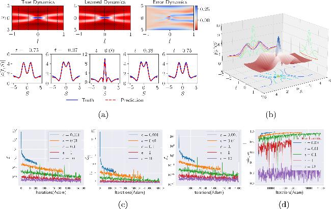
Figure 3. The training results of the second-order financial rogue wave φ(t, S) for the Ivancevic option pricing model arising from the RCPINN. (a) The ground truth, prediction and error dynamics density plots, as well as sectional drawings which contain the true and predicted second-order financial rogue wave at five distinct moments; (b) the three-dimensional plot with contour map for the predicted second-order financial rogue wave; (c) the evolution curve figures of three loss functions with different causality parameters during network training; (d) the evolution curve graph of minimal residual weights ${{\rm{\min }}}_{i}\,{w}_{i}$ during network training. |
Table 2. The comprehensive training results for predicting the second-order financial rogue wave. |
| ε | Adam | ${ \mathcal L }$ | ${{ \mathcal L }}_{ic}$ | ${{ \mathcal L }}_{r}$ | ${{\rm{\min }}}_{i}\,{w}_{i}$ |
|---|---|---|---|---|---|
| 10−3 | 13 300 | 2.0273e-01 | 1.4244e-04 | 1.8933e-01 | 0.9907 |
| 10−2 | 35 000 | 2.1247e-02 | 2.2069e-05 | 1.9053e-02 | 0.9906 |
| 10−1 | 50 000 | 1.4906e-02 | 1.3095e-05 | 1.3597e-02 | 0.9337 |
| 100 | 50 000 | 6.8507e-03 | 8.9566e-06 | 5.9259e-03 | 0.7459 |
| 101 | 50 000 | 2.5188e-03 | 7.1972e-06 | 1.8130e-03 | 0.4279 |
3.2. European option prices of nonlinear BS transaction-cost model
In the previous subsection, we successfully predicted the first-order and second-order financial rogue waves of the Ivancevic option pricing model by employing the RCPINN with two different initial data. In this part, we numerically predict and provide two different types of European option prices for the nonlinear BS transaction-cost model by means of the RCPINN with three different sets of initial data.
• European call option price
Unlike the traditional linear BS model, nonlinear BS models take into account more intricate market factors, such as transaction costs, market liquidity, and volatility variations. By incorporating nonlinear terms or stochastic components, these nonlinear models can provide a more realistic representation of market dynamics, thereby enabling the pricing of European options. In this part, we take the nonlinear BS transaction-cost model as the benchmark and employ an advanced deep learning algorithm, namely the RCPINN, together with a small set of initial data points, to predict or infer the evolution dynamics of two European call option prices, thereby providing a reference for practical market investments. We refer to [34], then consider the initial condition in the domain [0.01, 1] × [0, 1]
$\begin{eqnarray}\begin{array}{r}{ \mathcal I }(S)=1+\frac{0.5{\sigma }^{2}}{2\rho {\sigma }^{2}}S\left(1-{\mathrm{log}}S\right),\quad S\in [0.01,1].\end{array}\end{eqnarray}$
Once we set parameters r = 1, ρ = 0.1, σ = 1 in nonlinear BS transaction-cost model and initial condition (3.7 ). Then utilizing the initial condition (3.7 ), we select Nic = 512 initial training points and Nc = NtNS residual collocation points for the RCPINN. After setting 30 000 iterations of the Adam optimizer and using threshold δ = 0.99 to stop training, we successfully predicted the dynamics of the first kind of European call option price of nonlinear BS models by using the RCPINN, here the relative L2 norm error of the solution V(t, S) is 6.275e-03, and the training time of the network is 309.5550 s.
Figure 4 displays the training results of the predicted first kind of European call option price for the nonlinear BS transaction-cost model stemming from the RCPINN. Similarly, the abundant density plots and sectional drawings are revealed in figure 4(a), it can be observed that error occur at the right boundary of the underlying stock price, and these error become more pronounced as time increases. The three-dimensional plots and its contour map on three planes for the predicted first kind of European call option price are exhibited in figure 4(b). Then figure 4(c) reveals the loss function curves under different causality parameters, including the total loss function (${ \mathcal L }$) curve, initial condition loss function (${{ \mathcal L }}_{ic}$) curve and weighted residual loss function (${{ \mathcal L }}_{r}$) curve. Figure 4(d) presents the evolution curve graph of minimal residual weights during network training. Specifically, under the first three causal parameter conditions, ${{\rm{\min }}}_{i}\,{w}_{i}$ satisfied the stopping criterion, and under the latter two conditions, ${{\rm{\min }}}_{i}\,{w}_{i}$ was nearly close to it, thereby considerably enhancing the efficiency and accuracy of the network training. Finally, we provide the comprehensive training results for predicting the first kind of European call option price in table 3. Table 3 reports the detailed numerical results of the number of iterations, the three loss functions, and the minimum residual weights obtained under different causal parameter conditions.
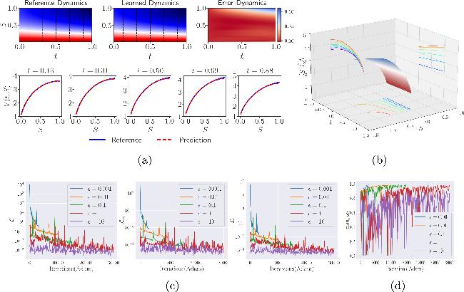
Figure 4. The training results of the first kind of European call option price V(t, S) for the nonlinear BS transaction-cost model arising from the RCPINN. (a) The reference, prediction and error dynamics density plots, as well as sectional drawings which contain the reference and predicted European call option price at five distinct moments; (b) the three-dimensional plot with contour map for the predicted European call option price; (c) the evolution curve figures of three loss functions with different causality parameters during network training; (d) the evolution curve graph of minimal residual weights ${{\rm{\min }}}_{i}\,{w}_{i}$ during network training. |
Table 3. The comprehensive training results for predicting the first kind of European call option price. |
| ε | Adam | ${ \mathcal L }$ | ${{ \mathcal L }}_{ic}$ | ${{ \mathcal L }}_{r}$ | ${{\rm{\min }}}_{i}\,{w}_{i}$ |
|---|---|---|---|---|---|
| 10−3 | 3200 | 2.5450e-01 | 8.3916e-05 | 1.7149e-01 | 0.9916 |
| 10−2 | 10 100 | 2.3866e-02 | 7.0323e-06 | 1.6843e-02 | 0.9918 |
| 10−1 | 15 200 | 2.3789e-03 | 7.6669e-07 | 1.6021e-03 | 0.9924 |
| 100 | 30 000 | 1.9504e-03 | 9.0539e-07 | 1.0470e-03 | 0.9506 |
| 101 | 30 000 | 6.4601e-04 | 2.0238e-07 | 4.4018e-04 | 0.8061 |
Furthermore, according to [34], we consider more complex initial condition within the domain [0.01, 1] × [0, 1], as presented below 3.8 ) is more complex than initial condition (3.7 ). Similarly, we set parameters r = 0.3, ρ = 0.1, σ = 1, ϵ = 1, δ = 1, k = 0.1 in nonlinear BS transaction-cost model and initial condition (3.8 ). From aforementioned initial condition (3.8 ), we select Nic = 512 initial points and Nc = NtNS residual collocation points for training of the RCPINN. Since the initial condition is more complex, the maximum number of iterations of the Adam optimizer for network training is set to 50 000 under different causal parameter conditions, while the stopping criterion threshold δ remains the same as before. After completing Adam optimization in the RCPINN, the relative L2 norm error reaches 4.932e-03 in 342.9251 s.
$\begin{eqnarray}\begin{array}{l}{ \mathcal I }(S)=\frac{rS}{\rho {\sigma }^{2}}\left[1-\frac{0.5{\sigma }^{2}}{2r}{\mathrm{log}}S+\frac{1}{2k}(\delta \sqrt{1-4\varepsilon {k}^{2}}-1){\mathrm{log}}S\right],\\ S\in [0.01,1].\end{array}\end{eqnarray}$
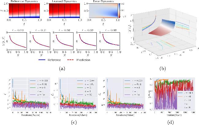
Evidently, although their mathematical forms are quite similar, initial condition (The training results of the second kind of European call option price stemming from the RCPINN are indicated in figure 5, in which figure 5(a) displays the abundant density plots and sectional drawings. In comparison with the first kind of European call option price illustrated in figure 4(a), figure 5(a) showcases that the network-predicted second kind of European call option price experiences a sharper increase over the same time horizon, which implies a greater potential for returns. While figure 5(b) displays the three-dimensional plot and its contour map on three planes for the predicted second kind of European call option price. Figure 5(c) shows the total loss function evolution curve figure, initial loss function evolution curve figure, and weighted residual loss function evolution curve figure during network training, respectively. The evolution curve graph of minimal residual weights ${{\rm{\min }}}_{i}\,{w}_{i}$ is displayed in figure 5(d). Table 4 exhibits a detailed training results for predicting the second kind of European call option price. By combining table 4 and figure 5(d), it can be observed that under the first four causal parameter conditions, the minimum weights ${{\rm{\min }}}_{i}\,{w}_{i}$ satisfied the stopping criterion, which substantially improved the efficiency and accuracy of network training while fully respecting the temporal causal structure.
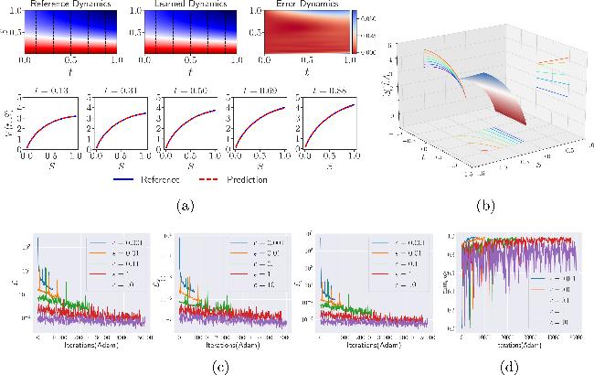
Figure 5. The training results of the second kind of European call option price V(t, S) for the nonlinear BS transaction-cost model arising from the RCPINN. (a) The reference, prediction and error dynamics density plots, as well as sectional drawings which contain the reference and predicted European call option price at five distinct moments; (b) the three-dimensional plot with contour map for the predicted European call option price; (c) the evolution curve figures of three loss functions with different causality parameters during network training; (d) the evolution curve graph of minimal residual weights ${{\rm{\min }}}_{i}\,{w}_{i}$ during network training. |
Table 4. The comprehensive training results for predicting the second kind of European call option price. |
| ε | Adam | ${ \mathcal L }$ | ${{ \mathcal L }}_{ic}$ | ${{ \mathcal L }}_{r}$ | ${{\rm{\min }}}_{i}\,{w}_{i}$ |
|---|---|---|---|---|---|
| 10−3 | 6900 | 2.4658e-01 | 4.9765e-05 | 1.9767e-01 | 0.9904 |
| 10−2 | 10 100 | 2.4365e-02 | 6.0044e-06 | 1.8344e-02 | 0.9915 |
| 10−1 | 23 900 | 2.6346e-03 | 5.5443e-07 | 2.1121e-03 | 0.9900 |
| 100 | 47 700 | 2.6203e-04 | 1.2085e-07 | 2.0105e-04 | 0.9903 |
| 101 | 50 000 | 1.0763e-03 | 8.6238e-08 | 9.6960e-04 | 0.6258 |
• European put option price
In contrast to the European call option, the European put option refers to the right to sell an asset with the pay-off function V(t, S). Both types of options are of great importance to investors, as they can minimize the losses caused by fluctuations in the underlying asset price. In this part, based on [34], we further consider the following initial condition 3.9 ). Here, the choice of the risk-free interest rate parameter r differs from that in the European call option case, a smaller value of r is selected in this case, which makes the network training more challenging. We adopt 512 initial points from initial condition, as well as Nc = NtNS residual collocation points in the RCPINN. Then, by using the Adam optimizer with a maximum of 50 000 iterations to address more complex training tasks, we obtain the 1.114e-02 relative L2 norm error for the predicted European put option price in 416.292564 s.
$\begin{eqnarray}{ \mathcal I }(S)=1+\frac{rS}{\rho {\sigma }^{2}}\left(1-\frac{0.5{\sigma }^{2}}{2r}{\mathrm{log}}S\right),\quad S\in [0.01,1].\end{eqnarray}$
Accordingly, the parameters are specified as r = 0.2, ρ = 0.1, σ = 1, k = 0.2 in nonlinear BS transaction-cost model and initial condition (Figure 6 displays the predicted European put option price V(t, S) by utilizing the RCPINN with the initial conditions of the nonlinear BS transaction-cost model. The upper panel of figure 6(a) depicts various dynamic density plots, including reference, learned dynamics as well as error dynamics with corresponding amplitude scale size on the right side, and the bottom panel of figure 6(a) presents sectional drawing at different moments. From figure 6(a), we can observe that the errors of the European put option price V(t, S) are relatively large when the time t is long and the underlying asset S is in the middle range. The three-dimensional plot with contour map on three planes for the predicted European put option price has been displayed in figure 6(b). The evolution curve figures of three different loss functions arising from the RCPINN are displayed in figure 6(c). Figure 6(d) exhibits the evolution of the minimum weight parameters ${{\rm{\min }}}_{i}\,{w}_{i}$ during network training under different causal parameter settings. It can be seen that, under the last two causal parameter conditions (ϵ = 1, 10), the two evolution curve graphs exhibit pronounced oscillations, indicating that network training is particularly challenging. Similarly, we exhibit that comprehensive training results for predicting the European put option price in table 5. Compared with the numerical results for the European call option in tables 3 and 4, we find that under the last three causal parameter settings (ϵ = 0.1, 1, 10), both the residual loss function and the total loss function of the network remain at the order of e-3. This further indicates that network training in this case is more challenging, partly due to the smaller risk-free rate parameter r and partly because the predicted European put option price is inherently more complex than the predicted European call option price.
Figure 6. The training results of the European put option price V(t, S) for the nonlinear BS transaction-cost model arising from the RCPINN. (a) The reference, prediction and error dynamics density plots, as well as sectional drawings which contain the reference and predicted European put option price at five distinct moments; (b) the three-dimensional plot with contour map for the predicted European put option price; (c) the evolution curve figures of three loss functions with different causality parameters during network training; (d) the evolution curve graph of minimal residual weights ${{\rm{\min }}}_{i}\,{w}_{i}$ during network training. |
Table 5. The comprehensive training results for predicting the European put option price. |
| ε | Adam | ${ \mathcal L }$ | ${{ \mathcal L }}_{ic}$ | ${{ \mathcal L }}_{r}$ | ${{\rm{\min }}}_{i}\,{w}_{i}$ |
|---|---|---|---|---|---|
| 10−3 | 5800 | 1.9895e-01 | 3.4828e-05 | 1.6473e-01 | 0.9919 |
| 10−2 | 17 900 | 2.0870e-02 | 1.9470e-06 | 1.8868e-02 | 0.9909 |
| 10−1 | 46 000 | 2.5624e-03 | 7.6255e-07 | 1.7173e-03 | 0.9915 |
| 100 | 50 000 | 6.4960e-03 | 1.9363e-07 | 6.3903e-03 | 0.7302 |
| 101 | 50 000 | 1.7182e-03 | 2.9247e-07 | 1.5297e-03 | 0.4748 |
In this section, by employing the RCPINN together with the corresponding initial data, we successfully predicted the financial rogue waves of the Ivancevic option pricing model and the European option prices of the nonlinear BS transaction cost model, then we presented the detailed numerical results. These numerical experiments encompass several research challenges, including the reliance solely on initial data, the strong nonlinearity of the models, the sensitivity to variations in initial data and the presence of small-scale model parameters. The numerical results indicate that, owing to it respects the inherent spatiotemporal causal structure of physical system evolution and other enhancement techniques, the RCPINN can overcome these research challenges and successfully predict financial rogue waves and European option prices.
4. Conclusions
This study addresses practical needs in financial markets and option pricing theory by innovatively applying the state of the art RCPINN to predict extreme rogue wave phenomena and European option prices in financial markets. We select the Ivancevic option pricing model (for describing potential extreme financial phenomena) and nonlinear BS transaction cost model (for pricing European option prices) as our research model. Due to the inherent uncertainty of stock prices in real financial markets, obtaining actual future data for both stock prices and option prices remains particularly challenging. Therefore, unlike prior studies, this work presents the first successful prediction of extreme financial rogue waves and European option price evolution using the Ivancevic option pricing model and the nonlinear BS transaction cost model based solely on limited initial data, highlighting the potential of deep learning in financial risk management and option pricing theory. We also provide a comprehensive introduce of the RCPINN, by rigorously preserving the inherent spatiotemporal causal structure of physical system evolution, this deep learning method proves particularly effective for investigating complex tasks exhibiting high sensitivity to initial data, including strongly nonlinear, multi-scale, chaotic, or turbulent behaviors. Then, the schematic architecture of the RCPINN is exhibited, which comprehensively demonstrate both the core methodology and enhanced technical features.
Financial rogue waves represent precisely this type of complex nonlinear localized wave phenomenon, characterized by their abrupt emergence and disappearance, making them notoriously difficult to detect and predict. Under given initial conditions of the Ivancevic option pricing model, our RCPINN framework successfully predicts two canonical types of financial rogue waves (namely first-order and second-order financial rogue waves) at specified future time points t and stock prices S. Moreover, the nonlinear BS model poses numerical challenges due to its strong nonlinearity, the multiscale nature of the small parameter r, and the sensitivity of its variable coefficients to changes in the independent variables. Based on the nonlinear BS transaction cost model, we employed the RCPINN to successfully predict the price evolution and dynamic characteristics of both European call and put options, offering a novel approach to European option pricing. This study not only provides a novel research tool for predicting extreme rogue wave phenomena in financial markets and related fields, but also offers an effective method for the numerical prediction of European option price evolution and its nonlinear dynamics. Furthermore, it presents a new technical approach for extreme financial risk early-warning systems and holds significant practical value in applications such as forecasting European option price evolution, exchange rate fluctuations, liquidity crisis monitoring, market crash prevention, and derivative pricing.