


1. Introduction
Recent advances in quantum computing and quantum simulation have intensified the demand for a deeper understanding of non-equilibrium dynamics in open quantum systems [1–6]. Clarifying the role of noise in quantum evolution [1, 7–14] can guide the design of more efficient, context-aware error-correction protocols, such as quantum error mitigation [15]. Concurrently, experimental progress has enabled unprecedented control over dissipative processes, alongside the development of novel detection methods [16–22] and quantum simulation platforms [1–4, 23].
Historically, a general framework for open quantum systems was established by Caldeira and Leggett [24–26], building on the influence functional techniques introduced by Feynman and Vernon [27]. These methods are powerful when the system is relatively simple and the environment is Gaussian. Through sustained efforts, theories for open quantum systems have been extended to strongly correlated systems [5, 28–31]. However, these approaches are often restricted to semiclassical regimes or designed for the vicinity of a steady state.
Constructing a theoretical framework for solving the many-body Lindblad equation faces two clear challenges: the exponential growth of the Hilbert space due to proliferating many-body correlations, and the quadratic scaling of density-matrix dynamics with the Hilbert-space dimension. Earlier studies on early-time dissipative dynamics—such as those based on dissipative response theory [16–18]—suggest that simplifications can be achieved by focusing solely on physical observables. If dynamical relations among a closed set of observables can be established, the dissipative evolution may be reconstructed via a tractable set of differential equations. In fact, this kind of equations can be obtained as addressed in [32], where it explained a dissipation induced coherent dynamics.
In this work, we investigate the dissipative dynamics of a finite-temperature (FT) superfluid. The dynamics of a superfluid–normal–fluid mixture in a closed system has been previously formulated within the Zaremba—Nikuni—Griffin (ZNG) formalism [33], which builds on a Green's function approach and the Baym–Kadanoff approximations [34, 35]. In the ZNG equations, the coherent superfluid is described by the Gross–Pitaevskii equation, while the normal component is treated semiclassically via a Boltzmann equation. A key feature of ZNG is the inclusion of Beliaev and Landau damping as dissipation mechanisms. However, treating these processes explicitly introduces considerable numerical complexity, whereas neglecting them leads to unstable dynamics due to the absence of relaxation. Recent theoretical efforts for dissipative many-body systems [36], most of which are variations of the ZNG formalism with an underlying Boltzmann equation, often face a trade-off: while formally more accurate, they require uncontrolled numerical approximations to manage their computational complexity, leading to issues with both accuracy and efficiency. On the other hand, the two-fluid hydrodynamical description [37], originally proposed for 4He, is only applicable when local equilibrium (equivalently, local detailed balance) can be established [38, 39]. This condition requires that macroscopic motion be systematically slower than the local relaxation.
We show that externally imposed dissipation offers two important advantages in this context. First, when external dissipation dominates over Beliaev and Landau damping, the intricate contributions from the latter can be neglected, substantially simplifying the analysis of dissipative dynamics. Second, dissipation stabilizes the hydrodynamic equations derived from a density-matrix approach that closely aligns with the ZNG formalism. This implies that external dissipation can also stabilize the hydrodynamic description, without requiring strong intrinsic interactions within the system. For these reasons, we obtain a self-consistent set of dissipative quantum Liouville equations (DQLE) for the condensate and the reduced density matrices.
By neglecting correlation functions associated with Beliaev and Landau damping, the DQLE becomes closed [32]. We then introduce a hydrodynamic expansion scheme that differs from the conventional Wigner-transform approach. Truncating this expansion yields a closed set of dissipative hydrodynamic equations (DHE). Emergence of hydrodynamics requires fast relaxation rate compared with typical dynamical time, or from collective motions by integrability [40–46]. Here we stress that the hydrodynamical expansion in present context includes hydrodynamical expansion coefficients beyond second order contributions, which alters the stability condition for traditional hydrodynamics.
To test the effectiveness of the DHE, we perform a systematic comparison between the DQLE and the DHE at different truncation orders. This leads to two principal findings:
(1) The early-time discrepancy between the DQLE and the DHE can be systematically reduced by increasing the order of the hydrodynamic expansion. Although higher truncation orders do not compromise the stability of the DHE, a characteristic time scale t0 emerges beyond which such higher-order hydrodynamic descriptions exhibit significant deviations. Notably, the stability of the DHE is enhanced both at lower expansion orders and in the presence of stronger dissipation.
(2) In the hydrodynamic expansion, the high-order (≥2; note that all odd-order coefficients vanish due to symmetry) terms of the anomalous density matrix decay much faster than other quantities in dissipative dynamics. We therefore test an approximation by setting all high-order expansion coefficients of the anomalous density to zero. We find that this approximation can stabilize the dynamical evolution described by the DHE. When the hydrodynamic expansion order for the normal-fluid density matrix is increased, the approximation is refined. In general, the DHE are more stable and more accurate for larger dissipation and smaller interaction strength.
In summary, based on a dissipative quantum Liouville framework for a FT superfluid, we obtained a set of dissipative hydrodynamical equations via systematic hydrodynamic expansion. Our analysis reveals that external dissipation not only simplifies the treatment of damping processes but also stabilizes the resulting hydrodynamic equations. By keeping only the zeroth-order term in the hydrodynamic expansion of the anomalous density matrix, the truncated hydrodynamic equations show good stability and accuracy in predicting hydrodynamic quantities. These results offer a step toward a more first-principles hydrodynamic theory for dissipative quantum fluids and suggest promising directions for the simulation and control of open quantum dynamics in complex settings, while greatly reducing the algorithmic complexity for accessing dissipative dynamics in an open system.
This article is organized as follows: In section 2 , we first derive the DQLE for a superfluid–normal–fluid mixture using a method inspired by dissipative response theory. In section 3 , we then introduce a systematic hydrodynamic expansion scheme, from which we obtain a set of DHE that incorporate the coherent condensate, squeezed states, and the normal fluid. In section 4 , we present numerical tests of both the DQLE and the DHE. By comparing the dynamical evolution across different approaches and at different hydrodynamic orders, we find that the most accurate and stable implementation of the DHE is achieved by retaining only the zeroth-order term in the hydrodynamic expansion for the anomalous density function, while setting all second-order and higher expansion coefficients to zero. Within this scheme, we observe that the hydrodynamic description becomes particularly effective—yielding results in close agreement with the full DQLE—when the external dissipation is strong and the inter-particle interaction is weak.
2. Dissipative quantum Liouville equations for weakly interacting bosons
We study a system of weakly interacting bosons described by the grand canonical Hamiltonian 1 ) and (2 ) reads
$\begin{eqnarray}\begin{array}{rcl}\hat{H} & = & \displaystyle \int \,{\rm{d}}{\boldsymbol{r}}\,{\hat{\psi }}^{\dagger }({\boldsymbol{r}},t){\hat{h}}_{0}({\boldsymbol{r}})\hat{\psi }({\boldsymbol{r}},t)\\ & & +\frac{1}{2}\,\displaystyle \int \,{\rm{d}}{\boldsymbol{r}}\displaystyle \int \,{\rm{d}}{{\boldsymbol{r}}}^{{\prime} }{\hat{\psi }}^{\dagger }({\boldsymbol{r}},t){\hat{\psi }}^{\dagger }({{\boldsymbol{r}}}^{{\prime} },t)\\ & & \times V({\boldsymbol{r}}-{{\boldsymbol{r}}}^{{\prime} })\hat{\psi }({\boldsymbol{r}},t)\hat{\psi }({{\boldsymbol{r}}}^{{\prime} },t),\end{array}\end{eqnarray}$
where the single-particle Hamiltonian is given by ${\hat{h}}_{0}({\boldsymbol{r}})\,=-\frac{{\hslash }^{2}}{2m}{{\rm{\nabla }}}^{2}+{V}_{{\rm{ext}}}({\boldsymbol{r}})-\mu $, and the field operators satisfy the equal-time commutation relation $[\hat{\psi }({\boldsymbol{r}},t),{\hat{\psi }}^{\dagger }({{\boldsymbol{r}}}^{{\prime} },t)]\,=\delta ({\boldsymbol{r}}-{{\boldsymbol{r}}}^{{\prime} })$. In a dilute Bose gas at temperatures well below the condensation temperature, the interatomic potential can be approximated by a local contact interaction, $\begin{eqnarray}V({\boldsymbol{r}}-{{\boldsymbol{r}}}^{{\prime} })=g\delta ({\boldsymbol{r}}-{{\boldsymbol{r}}}^{{\prime} }),\end{eqnarray}$
where g satisfies renormalization condition g = 4πℏ2as/m. Here as denotes the s-wave scattering length. The Heisenberg equation of motion for the field operator derived from equations ( $\begin{eqnarray}{\rm{i}}\hslash {\partial }_{t}\hat{\psi }({\boldsymbol{r}},t)={\hat{h}}_{0}({\boldsymbol{r}})\hat{\psi }({\boldsymbol{r}},t)+g{\hat{\psi }}^{\dagger }({\boldsymbol{r}},t)\hat{\psi }({\boldsymbol{r}},t)\hat{\psi }({\boldsymbol{r}},t).\end{eqnarray}$
2.1. Quantum Liouville equations
Here we will first review the method introduced in [32] for establishing the DQLE. To incorporate dissipative and fluctuation effects beyond the mean-field approximation, we decompose the field operator into a macroscopic wavefunction (the condensate order parameter) and a fluctuation operator:
$\begin{eqnarray}\hat{\psi }({\boldsymbol{r}},t)={\rm{\Phi }}({\boldsymbol{r}},t)+\delta \hat{\phi }({\boldsymbol{r}},t),\end{eqnarray}$
with ${\rm{\Phi }}({\boldsymbol{r}},t)=\langle \hat{\psi }({\boldsymbol{r}},t)\rangle $ and $\langle \delta \hat{\phi }({\boldsymbol{r}},t)\rangle =0$. The system dynamics are then governed by the evolution of Φ(r, t) and the non-condensate correlation functions, such as the normal density matrix ${\rho }^{\lt }({\boldsymbol{r}},{{\boldsymbol{r}}}^{{\prime} },t)=\langle \delta {\hat{\phi }}^{\dagger }({\boldsymbol{r}},t)\delta \hat{\phi }({{\boldsymbol{r}}}^{{\prime} },t)\rangle $, the anomalous density matrix ${\rho }_{A}({\boldsymbol{r}},{{\boldsymbol{r}}}^{{\prime} },t)=\langle \delta \hat{\phi }({\boldsymbol{r}},t)\delta \hat{\phi }({{\boldsymbol{r}}}^{{\prime} },t)\rangle $, and the complementary normal density ${\rho }^{\gt }({{\boldsymbol{r}}}^{{\prime} },{\boldsymbol{r}};t)=\langle \delta {\hat{\phi }}^{}({{\boldsymbol{r}}}^{{\prime} },t)\delta {\hat{\phi }}^{\dagger }({\boldsymbol{r}},t)\rangle $. Note that ρ< corresponds to the one-particle reduced density matrix ρ. Here we assume ${\boldsymbol{r}}={{\boldsymbol{r}}}^{{\prime} }$ is defined as a continuous limit of ${\boldsymbol{r}}-{{\boldsymbol{r}}}^{{\prime} }\to 0$, then we find ${\rho }^{\lt }({\boldsymbol{r}},{{\boldsymbol{r}}}^{{\prime} };t)={\rho }^{\gt }({{\boldsymbol{r}}}^{{\prime} },{\boldsymbol{r}};t)$. For this reason, we introduce $\rho ({\boldsymbol{r}},{{\boldsymbol{r}}}^{{\prime} };t)={\rho }^{\lt }({\boldsymbol{r}},{{\boldsymbol{r}}}^{{\prime} };t)={\rho }^{\gt }({{\boldsymbol{r}}}^{{\prime} },{\boldsymbol{r}};t)$ to eliminate the complexity.The mean-field decomposition leads to a closed set of dynamical equations for the condensate order parameter Φ(r, t) and the fluctuation operator $\delta \hat{\phi }({\boldsymbol{r}},t)$. The evolution of the condensate is governed by a generalized Gross–Pitaevskii equation:
$\begin{eqnarray}\begin{array}{rcl}{\rm{i}}\hslash {\partial }_{t}{\rm{\Phi }}({\boldsymbol{r}},t) & = & {\hat{h}}_{0}({\boldsymbol{r}}){\rm{\Phi }}+g| {\rm{\Phi }}{| }^{2}{\rm{\Phi }}+2g\rho ({\boldsymbol{r}},{\boldsymbol{r}};t){\rm{\Phi }}\\ & & +g{\rho }_{A}({\boldsymbol{r}},{\boldsymbol{r}};t){{\rm{\Phi }}}^{* }.\end{array}\end{eqnarray}$
This equation extends the standard GPE by including two FT contributions. Concurrently, the fluctuations evolve according to a Bogoliubov–de Gennes-type equation, $\begin{eqnarray}\begin{array}{rcl}{\rm{i}}\hslash {\partial }_{t}\delta \hat{\phi }({\boldsymbol{r}},t) & = & \left(-\frac{{\hslash }^{2}}{2m}{{\rm{\nabla }}}_{{\boldsymbol{r}}}^{2}+{V}_{{\rm{eff}}}({\boldsymbol{r}},t)-\mu \right)\\ & & \times \delta \hat{\phi }+{V}_{A}({\boldsymbol{r}},t)\delta {\hat{\phi }}^{\dagger },\end{array}\end{eqnarray}$
where the effective potential and anomalous potential are self-consistently defined as $\begin{eqnarray}{V}_{{\rm{eff}}}({\boldsymbol{r}},t)\equiv {V}_{{\rm{ext}}}({\boldsymbol{r}})+2g\left[| {\rm{\Phi }}({\boldsymbol{r}},t){| }^{2}+\rho ({\boldsymbol{r}},{\boldsymbol{r}};t)\right],\end{eqnarray}$
$\begin{eqnarray}{V}_{A}({\boldsymbol{r}},t)\equiv g\left[{{\rm{\Phi }}}^{2}({\boldsymbol{r}},t)+{\rho }_{A}({\boldsymbol{r}},{\boldsymbol{r}};t)\right].\end{eqnarray}$
In this framework, Veff acts as a dynamic trapping potential for the excitations, while VA governs the coherent creation and annihilation of quasiparticle pairs. A similar equation can be written for $\delta {\hat{\phi }}^{\dagger }({\boldsymbol{r}},t)$. In the above expressions, we have neglected the expectation value $\langle \delta {\hat{\phi }}^{\dagger }\delta \hat{\phi }\delta \hat{\phi }\rangle $, which accounts for Beliaev and Landau damping processes. At the single-particle level, this term corresponds to the imaginary part of ${g}^{2}\langle \delta {\hat{\phi }}^{\dagger }({\boldsymbol{r}},t)\delta \phi ({\boldsymbol{r}},t)\rangle $.Neglecting dissipative effects arising from interactions—which is justified for weakly interacting systems—we focus on the dynamics of Φ(r, t) and the correlation functions $\rho ({\boldsymbol{r}},{{\boldsymbol{r}}}^{{\prime} };t)$ and ${\rho }_{A}({\boldsymbol{r}},{{\boldsymbol{r}}}^{{\prime} };t)$. Starting from the definitions $\rho ({\boldsymbol{r}},{{\boldsymbol{r}}}^{{\prime} };t)\,=\langle \delta {\hat{\phi }}^{\dagger }({\boldsymbol{r}},t)\delta \hat{\phi }({{\boldsymbol{r}}}^{{\prime} },t)\rangle $ and ${\rho }_{A}({\boldsymbol{r}},{{\boldsymbol{r}}}^{{\prime} },t)=\langle \delta \hat{\phi }({\boldsymbol{r}},t)\delta \hat{\phi }({{\boldsymbol{r}}}^{{\prime} },t)\rangle $, the time evolution is given by
$\begin{eqnarray}\begin{array}{rcl}{\rm{i}}\hslash {\partial }_{t}\rho ({\boldsymbol{r}},{{\boldsymbol{r}}}^{{\prime} };t) & = & \frac{{\hslash }^{2}}{2m}({{\rm{\nabla }}}_{{\boldsymbol{r}}}^{2}-{{\rm{\nabla }}}_{{{\boldsymbol{r}}}^{{\prime} }}^{2})\rho ({\boldsymbol{r}},{{\boldsymbol{r}}}^{{\prime} };t)\\ & & -\left[{V}_{{\rm{eff}}}({\boldsymbol{r}},t)-{V}_{{\rm{eff}}}({{\boldsymbol{r}}}^{{\prime} },t)\right]\rho ({\boldsymbol{r}},{{\boldsymbol{r}}}^{{\prime} };t)\\ & & -{V}_{A}^{* }({\boldsymbol{r}},t){\rho }_{A}({\boldsymbol{r}},{{\boldsymbol{r}}}^{{\prime} };t)\\ & & +{V}_{A}({{\boldsymbol{r}}}^{{\prime} },t){\rho }_{A}^{* }({{\boldsymbol{r}}}^{{\prime} },{\boldsymbol{r}};t),\end{array}\end{eqnarray}$
$\begin{eqnarray}\begin{array}{rcl}{\rm{i}}\hslash {\partial }_{t}{\rho }_{A}({\boldsymbol{r}},{{\boldsymbol{r}}}^{{\prime} };t) & = & -\frac{{\hslash }^{2}}{2m}({{\rm{\nabla }}}_{{\boldsymbol{r}}}^{2}+{{\rm{\nabla }}}_{{{\boldsymbol{r}}}^{{\prime} }}^{2}){\rho }_{A}({\boldsymbol{r}},{{\boldsymbol{r}}}^{{\prime} };t)\\ & & +[{V}_{{\rm{eff}}}({\boldsymbol{r}},t)+{V}_{{\rm{eff}}}({{\boldsymbol{r}}}^{{\prime} },t)-2\mu ]\\ & & \times {\rho }_{A}({\boldsymbol{r}},{{\boldsymbol{r}}}^{{\prime} };t)\\ & & +{V}_{A}({\boldsymbol{r}},t)\rho ({\boldsymbol{r}},{{\boldsymbol{r}}}^{{\prime} };t)\\ & & +{V}_{A}({{\boldsymbol{r}}}^{{\prime} },t)\rho ({{\boldsymbol{r}}}^{{\prime} },{\boldsymbol{r}};t).\end{array}\end{eqnarray}$
These equations are formulated in the Schrödinger picture and can be interpreted as quantum Liouville equations for generalized density matrices.2.2. Dissipative dynamics in the normal state
For dissipative systems, the dynamics can be described within the framework of dissipative response theory. For any physical observable $\hat{{ \mathcal W }}$, such as $\hat{\rho }({\boldsymbol{r}},{{\boldsymbol{r}}}^{{\prime} };t)$ or ${\hat{\rho }}_{A}({\boldsymbol{r}},{{\boldsymbol{r}}}^{{\prime} };t)$, we have
$\begin{eqnarray}\begin{array}{rcl}\delta \hat{{ \mathcal W }}(t) & = & \gamma {\displaystyle \int }_{0}^{t}{\rm{d}}{t}^{{\prime} }\displaystyle \sum _{j}\left(\right.{\hat{{ \mathcal O }}}_{j}^{\dagger }({t}^{{\prime} })\hat{{ \mathcal W }}(t){\hat{{ \mathcal O }}}_{j}({t}^{{\prime} })\\ & & -\frac{1}{2}\{{\hat{{ \mathcal O }}}_{j}^{\dagger }({t}^{{\prime} }){\hat{{ \mathcal O }}}_{j}({t}^{{\prime} }),\hat{{ \mathcal W }}(t)\}\left)\right.,\end{array}\end{eqnarray}$
where $\hat{{ \mathcal W }}(t)$ and ${\hat{{ \mathcal O }}}_{j}(t)$ are in the interaction picture. Since this relation holds at the operator level, the expectation value for any $\hat{{ \mathcal W }}$ satisfies $\begin{eqnarray}\frac{\delta { \mathcal W }}{\delta t}=\gamma \displaystyle \sum _{j}\left\langle {{ \mathcal L }}_{{\hat{{ \mathcal O }}}_{j}}(\hat{{ \mathcal W }})(t)\right\rangle ,\end{eqnarray}$
with $\left\langle \cdots \,\right\rangle ={\rm{Tr}}(\rho \cdots \,)$ denoting the average over the density matrix state, and $\begin{eqnarray}{{ \mathcal L }}_{{\hat{{ \mathcal O }}}_{j}}(\hat{{ \mathcal W }})={\hat{{ \mathcal O }}}_{j}^{\dagger }\hat{{ \mathcal W }}{\hat{{ \mathcal O }}}_{j}-\frac{1}{2}\{{\hat{{ \mathcal O }}}_{j}^{\dagger }{\hat{{ \mathcal O }}}_{j},\hat{{ \mathcal W }}\}\end{eqnarray}$
defining the Lindblad superoperator. Here ${\hat{{ \mathcal O }}}_{j}$ represents the dissipation operator. In the Heisenberg picture, the dynamical equation becomes $\begin{eqnarray}\frac{{\rm{d}}{ \mathcal W }(t)}{{\rm{d}}t}=\frac{1}{{\rm{i}}\hslash }\left\langle [\hat{{ \mathcal W }},\hat{H}]\right\rangle (t)+\gamma \displaystyle \sum _{j}\left\langle {{ \mathcal L }}_{{\hat{{ \mathcal O }}}_{j}}(\hat{{ \mathcal W }})\right\rangle (t).\end{eqnarray}$
In general, the operators $[\hat{{ \mathcal W }},\hat{H}]$ and ${\sum }_{j}{{ \mathcal L }}_{{\hat{{ \mathcal O }}}_{j}}(\hat{{ \mathcal W }})$ are not solely functions of $\hat{{ \mathcal W }}$. However, when the expectation values $\langle [\hat{{ \mathcal W }},\hat{H}]\rangle $ and ${\sum }_{j}\langle {{ \mathcal L }}_{{\hat{{ \mathcal O }}}_{j}}(\hat{{ \mathcal W }})\rangle $ can be factorized into products of expectation values $\langle {\hat{{ \mathcal W }}}_{\ell }\rangle (t)$, and the relevant observables in the dynamical equations for each $\langle {\hat{{ \mathcal W }}}_{\ell }\rangle (t)$ form a closed set, one obtains a self-consistent system of coupled dynamical equations.For the case of single-particle loss where the dissipation acts uniformly on all particles in the normal state, i.e. ${\hat{{ \mathcal O }}}_{j}\to \delta \hat{\phi }({{\boldsymbol{r}}}_{1})$, we find 5 ), (16 ) and (17 ) form a closed system for the condensate wavefunction Φ(r, t), the normal density matrix $\rho ({\boldsymbol{r}},{{\boldsymbol{r}}}^{{\prime} };t)$, and the anomalous density matrix ${\rho }_{A}({\boldsymbol{r}},{{\boldsymbol{r}}}^{{\prime} };t)$, which we refer to as the DQLE.
$\begin{eqnarray}\begin{array}{rcl}{{ \mathcal L }}_{\delta \hat{\phi }({{\boldsymbol{r}}}_{1})}(\hat{\rho }) & = & -\frac{1}{2}\left[\delta ({{\boldsymbol{r}}}_{1}\,-\,{\boldsymbol{r}})\hat{\rho }({{\boldsymbol{r}}}_{1},{{\boldsymbol{r}}}^{{\prime} })\,+\,\delta ({{\boldsymbol{r}}}_{1}\,-\,{{\boldsymbol{r}}}^{{\prime} })\hat{\rho }({\boldsymbol{r}},{{\boldsymbol{r}}}_{1})\right],\\ {{ \mathcal L }}_{\delta \hat{\phi }({{\boldsymbol{r}}}_{1})}({\hat{\rho }}_{A}) & = & -\frac{1}{2}\left[\delta ({{\boldsymbol{r}}}_{1}\,-\,{\boldsymbol{r}}){\hat{\rho }}_{A}({{\boldsymbol{r}}}_{1},{{\boldsymbol{r}}}^{{\prime} })\,+\,\delta ({{\boldsymbol{r}}}_{1}\,-\,{{\boldsymbol{r}}}^{{\prime} }){\hat{\rho }}_{A}({\boldsymbol{r}},{{\boldsymbol{r}}}_{1})\right].\end{array}\end{eqnarray}$
Consequently, the equation of motion for the normal density matrix becomes $\begin{eqnarray}\begin{array}{rcl}{\rm{i}}\hslash {\partial }_{t}\rho & = & \frac{{\hslash }^{2}}{2m}({{\rm{\nabla }}}_{{\boldsymbol{r}}}^{2}-{{\rm{\nabla }}}_{{{\boldsymbol{r}}}^{{\prime} }}^{2})\rho -({V}_{{\rm{eff}}}\rho -\rho {V}_{{\rm{eff}}})\\ & & -({V}_{A}^{* }{\rho }_{A}-{\rho }_{A}^{* }{V}_{A})-{\rm{i}}\hslash \gamma \rho ,\end{array}\end{eqnarray}$
where we employ the convention ${V}_{{\rm{eff}}}\rho \equiv {V}_{{\rm{eff}}}({\boldsymbol{r}},t)\rho ({\boldsymbol{r}},{{\boldsymbol{r}}}^{{\prime} };t)$ and $\rho {V}_{{\rm{eff}}}\equiv \rho ({\boldsymbol{r}},{{\boldsymbol{r}}}^{{\prime} };t){V}_{{\rm{eff}}}({{\boldsymbol{r}}}^{{\prime} },t)$. This notation facilitates generalization to systems with internal degrees of freedom. Similarly, the equation for the anomalous density matrix is $\begin{eqnarray}\begin{array}{rcl}{\rm{i}}\hslash {\partial }_{t}{\rho }_{A} & = & -\frac{{\hslash }^{2}}{2m}({{\rm{\nabla }}}_{{\boldsymbol{r}}}^{2}+{{\rm{\nabla }}}_{{{\boldsymbol{r}}}^{{\prime} }}^{2}){\rho }_{A}+\left({V}_{{\rm{eff}}}{\rho }_{A}+{\rho }_{A}{V}_{{\rm{eff}}}\right)\\ & & +\left({V}_{A}\rho +{\rho }^{T}{V}_{A}\right)-{\rm{i}}\hslash \gamma {\rho }_{A},\end{array}\end{eqnarray}$
with the products interpreted according to the same convention. The equations (The formalism naturally extends to other dissipative mechanisms. For example, two-particle loss, a prevalent process in ultracold atomic gases, is modeled by a jump operator quadratic in the field operators, ${\hat{{ \mathcal O }}}_{j}\to \delta \hat{\phi }({{\boldsymbol{r}}}_{1})\delta \hat{\phi }({{\boldsymbol{r}}}_{1})$. Within the same mean-field approximation, this process contributes the following terms to the equations of motion:
$\begin{eqnarray}\begin{array}{rcl}\frac{\delta \rho ({\boldsymbol{r}},{{\boldsymbol{r}}}^{{\prime} };t)}{\delta t} & = & -\gamma \left[2\rho ({\boldsymbol{r}},{\boldsymbol{r}};t)\rho ({\boldsymbol{r}},{{\boldsymbol{r}}}^{{\prime} };t)\right.\\ & & +{\rho }_{A}^{* }({\boldsymbol{r}},{\boldsymbol{r}};t){\rho }_{A}({\boldsymbol{r}},{{\boldsymbol{r}}}^{{\prime} };t)\\ & & +2\rho ({\boldsymbol{r}},{{\boldsymbol{r}}}^{{\prime} };t)\rho ({{\boldsymbol{r}}}^{{\prime} },{{\boldsymbol{r}}}^{{\prime} };t)\\ & & \left.+{\rho }_{A}^{* }({\boldsymbol{r}},{{\boldsymbol{r}}}^{{\prime} };t){\rho }_{A}({{\boldsymbol{r}}}^{{\prime} },{{\boldsymbol{r}}}^{{\prime} };t)\right],\end{array}\end{eqnarray}$
$\begin{eqnarray}\begin{array}{rcl}\frac{\delta {\rho }_{A}({\boldsymbol{r}},{{\boldsymbol{r}}}^{{\prime} };t)}{\delta t} & = & -\gamma \left[2\rho ({\boldsymbol{r}},{\boldsymbol{r}};t){\rho }_{A}({\boldsymbol{r}},{{\boldsymbol{r}}}^{{\prime} };t)\right.\\ & & +{\rho }_{A}({\boldsymbol{r}},{\boldsymbol{r}};t)\rho ({\boldsymbol{r}},{{\boldsymbol{r}}}^{{\prime} };t)\\ & & +2\rho ({{\boldsymbol{r}}}^{{\prime} },{{\boldsymbol{r}}}^{{\prime} };t){\rho }_{A}({\boldsymbol{r}},{{\boldsymbol{r}}}^{{\prime} };t)\\ & & \left.+{\rho }_{A}({{\boldsymbol{r}}}^{{\prime} },{{\boldsymbol{r}}}^{{\prime} };t)\rho ({{\boldsymbol{r}}}^{{\prime} },{\boldsymbol{r}};t)\right].\end{array}\end{eqnarray}$
These expressions illustrate how different dissipative processes modify the coherent dynamics of both normal and anomalous correlations in a many-body system.3. Hydrodynamical expansion and dissipative hydrodynamical equations
A key finding of this work is that, up to a certain dissipation strength, the hydrodynamic expansion of density matrices ρ and ρA provides a good approximation. To implement this, we introduce center-of-mass and relative coordinates:
$\begin{eqnarray}{\boldsymbol{R}}=\frac{{\boldsymbol{r}}+{{\boldsymbol{r}}}^{{\prime} }}{2},\quad {\boldsymbol{S}}={\boldsymbol{r}}-{{\boldsymbol{r}}}^{{\prime} }.\end{eqnarray}$
The density matrices can then be systematically expanded in a Taylor series in powers of the relative coordinate S, which acts as a small parameter. This procedure converts the original non-local two-point correlation functions into an infinite series of purely local hydrodynamic fields defined at the single coordinate R. For a general two-point function ${ \mathcal F }({\boldsymbol{r}},{{\boldsymbol{r}}}^{{\prime} };t)$ (representing either ρ or ρA), this expansion takes the form: $\begin{eqnarray}{ \mathcal F }({\boldsymbol{r}},{{\boldsymbol{r}}}^{{\prime} };t)={\left.\displaystyle \sum _{n=0}^{\infty }\frac{1}{n!}\left({S}_{{i}_{1}}\,\cdots {S}_{{i}_{n}}\right)\left[{\partial }_{{S}_{{i}_{1}}}\,\cdots {\partial }_{{S}_{{i}_{n}}}{ \mathcal F }({\boldsymbol{R}},{\boldsymbol{S}};t)\right]\right|}_{{\boldsymbol{S}}=0}.\end{eqnarray}$
Here, repeated spatial indices i1, i2, …, in are summed over, following Einstein's convention. This formalism establishes a direct bridge between the microscopic quantum description and the emergent coarse-grained hydrodynamic quantities.The zeroth-order expansion term (n = 0) of the normal density matrix $\rho ({\boldsymbol{r}},{{\boldsymbol{r}}}^{{\prime} };t)$ corresponds to the local density, ρ(R, t), defined as the density for finding a normal particle at position R and time t. In hydrodynamic terms, it describes the distribution of the thermal cloud and serves as the fundamental field for continuity equations. Proceeding to the first-order term, we obtain:
$\begin{eqnarray}{\left.{\partial }_{{S}_{i}}\rho ({\boldsymbol{R}},{\boldsymbol{S}};t)\right|}_{{\boldsymbol{S}}=0}\equiv \frac{m}{{\rm{i}}\hslash }{j}_{i}({\boldsymbol{R}},t),\end{eqnarray}$
which corresponds to the local current field. The second-order derivative yields the momentum flux or stress tensor: $\begin{eqnarray}{\left.{\partial }_{{S}_{i}}{\partial }_{{S}_{j}}\rho ({\boldsymbol{R}},{\boldsymbol{S}};t)\right|}_{{\boldsymbol{S}}=0}\equiv 2{\left(\frac{m}{{\rm{i}}\hslash }\right)}^{2}{\tau }_{ij}({\boldsymbol{R}},t).\end{eqnarray}$
This term encapsulates essential information about the kinetic energy density and the stress within the fluid. Expanding both density matrices up to the fourth-order in the relative coordinate S, we obtain the following explicit forms For the normal density matrix $\rho ({\boldsymbol{r}},{{\boldsymbol{r}}}^{{\prime} };t)$, the series reads: $\begin{eqnarray}\begin{array}{rcl}\rho ({\boldsymbol{r}},{{\boldsymbol{r}}}^{{\prime} };t) & = & \rho +\frac{m}{{\rm{i}}\hslash }{S}_{i}{j}_{i}+{\left(\frac{m}{{\rm{i}}\hslash }\right)}^{2}{S}_{i}{S}_{j}{\tau }_{ij}\\ & & +{\left(\frac{m}{{\rm{i}}\hslash }\right)}^{3}\,{S}_{i}{S}_{j}{S}_{k}{X}_{ijk}+{\left(\frac{m}{{\rm{i}}\hslash }\right)}^{4}{S}_{i}{S}_{j}{S}_{k}{S}_{l}{Y}_{ijkl}+\cdots \,,\end{array}\end{eqnarray}$
with summation over repeated spatial indices i, j, k, l = x, y, z. A critical observation is that, due to the Hermitian property of $\rho ({\boldsymbol{r}},{{\boldsymbol{r}}}^{{\prime} };t)$, all coefficients in this expansion—ρ, ji, τij, Xijk, Yijkl—are real-valued functions of R and t. Moreover, the coefficient multiplying the nth power of Si constitutes a fully symmetric rank-n tensor. That is, ρ is a scalar, ji a vector, τij a symmetric second-rank tensor (τij = τji), Xijk a fully symmetric third-rank tensor, and Yijkl a fully symmetric fourth-rank tensor. This complete permutation symmetry in the tensor indices stems from the Hermiticity condition and the symmetric nature of the product ${S}_{{i}_{1}}\cdots {S}_{{i}_{n}}$ in the expansion. For the anomalous density ρA, the exchange symmetry ${\rho }_{A}({\boldsymbol{r}},{{\boldsymbol{r}}}^{{\prime} };t)={\rho }_{A}({{\boldsymbol{r}}}^{{\prime} },{\boldsymbol{r}};t)$ implies that all odd-order terms in S must vanish. Consequently, its expansion contains only even powers: $\begin{eqnarray}{\rho }_{A}({\boldsymbol{r}},{{\boldsymbol{r}}}^{{\prime} };t)={\rho }^{A}+{\left(\frac{m}{{\rm{i}}\hslash }\right)}^{2}\,{S}_{i}{S}_{j}{\tau }_{ij}^{A}+{\left(\frac{m}{{\rm{i}}\hslash }\right)}^{4}\,{S}_{i}{S}_{j}{S}_{k}{S}_{l}{Y}_{ijkl}^{A}+\cdots \end{eqnarray}$
Structurally, the coefficients retain the same tensor symmetry as in the normal case: ρA is a scalar, ${\tau }_{ij}^{A}$ is symmetric in its indices (${\tau }_{ij}^{A}={\tau }_{ji}^{A}$), and ${Y}_{ijkl}^{A}$ is fully symmetric in all four indices. However, the coefficients ρA, ${\tau }_{ij}^{A}$, and ${Y}_{ijkl}^{A}$ are generally complex-valued functions of R and t. This reflects the fact that the anomalous density ρA is not Hermitian. The complex nature of these fields is essential for capturing phenomena such as superfluid phase dynamics and coherence in Bose-condensed systems.Within the same coordinate framework, functions that depend on only a single spatial variable, such as the condensate order parameter Φ(r, t), the effective potential Veff(r, t), and the anomalous potential VA(r, t), must also be expressed in terms of R and S to be consistent with the expansion of the two-point density matrices. For a generic single-point function ${ \mathcal G }({\boldsymbol{r}},t)$, the coordinate transformation r = R + S/2 leads to the Taylor expansion:
$\begin{eqnarray}{\left.{ \mathcal G }({\boldsymbol{r}},t)=\displaystyle \sum _{n=0}^{\infty }\frac{1}{n!}{\left(\frac{{\boldsymbol{S}}}{2}\cdot {{\rm{\nabla }}}_{{\boldsymbol{R}}}\right)}^{n}{ \mathcal G }\left({\boldsymbol{R}}+\frac{{\boldsymbol{S}}}{2};t\right)\right|}_{{\boldsymbol{S}}=0}.\end{eqnarray}$
Here, the expansion is performed around S = 0, meaning all derivatives of the function ${ \mathcal G }({\boldsymbol{r}},t)$ are evaluated at the center-of-mass coordinate R. By expanding the DQLE in this manner and comparing coefficients order by order in S, we subsequently derive a closed set of finite-order hydrodynamic equations.3.1. 2nd-order dissipative hydrodynamical equations for ρ and ρA
The objective of this section is to systematically derive the DHE, which describe the coarse-grained, non-equilibrium dynamics of a dissipative Bose gas. Upon expanding the density equations (16 ) and (17 ) within the DQLE framework, we obtain a hierarchy of hydrodynamic equations order by order in the relative coordinate S. Here we present the key results up to second order, which form a closed set of dynamical equations for the leading normal and anomalous hydrodynamic quantities. For brevity, we omit the explicit dependence on (R, t) for all expanded quantities.
The expansion of equation (16 ) yields the zeroth-order equation:
$\begin{eqnarray}({\partial }_{t}+\gamma )\rho +{\rm{\nabla }}\cdot {\boldsymbol{j}}=\frac{2g}{\hslash }{\rm{Im}}\left[{{\rm{\Phi }}}^{2}{\rho }^{A* }\right].\end{eqnarray}$
Introducing the polar representations Φ = ∣Φ∣eiθ and ρA = ∣ρA∣eiκ, we obtain $\begin{eqnarray}({\partial }_{t}+\gamma )\rho +{\rm{\nabla }}\cdot {\boldsymbol{j}}=\frac{2g}{\hslash }| {\rm{\Phi }}{| }^{2}| {\rho }^{A}| \sin (2\theta -\kappa ).\end{eqnarray}$
This equation represents a continuity equation modified by a coherent particle exchange term between the condensate and the normal fluid. The direction of particle flow is governed by the phase difference 2θ − κ: when 2θ − κ > 0, particles are gained by the normal fluid, corresponding to a loss from the condensate.The dynamical equation for the momentum density (or current) is obtained at first order. It governs the evolution of the current field ji and can be cast in the following form:
$\begin{eqnarray}({\partial }_{t}+\gamma ){j}_{i}=-2{\partial }_{j}{\tau }_{ij}^{{\rm{S}}}-\frac{\rho }{m}{\partial }_{i}{V}_{{\rm{eff}}}-\frac{1}{m}{\rm{Re}}\left[({\partial }_{i}{V}_{A}^{* }){\rho }^{A}\right],\end{eqnarray}$
where ${\tau }_{ij}^{{\rm{S}}}=({\tau }_{ij}+{\tau }_{ji})/2$. According to the symmetry of τij, we have ${\tau }_{ij}^{{\rm{S}}}={\tau }_{ij}$. Einstein sum rule is implied where repeated indices means summation. Defining the effective force density as fi = −∂iVeff and expressing the anomalous potential explicitly, the equation can be rewritten as $\begin{eqnarray}\begin{array}{rcl}({\partial }_{t}+\gamma ){j}_{i} & = & -2{\partial }_{j}{\tau }_{ij}^{{\rm{S}}}\\ & & +\frac{\rho }{m}{f}_{i}-\frac{g}{2m}{\partial }_{i}| {\rho }^{A}{| }^{2}-\frac{g}{m}{\rm{Re}}\left[{\partial }_{i}({{\rm{\Phi }}}^{* 2}){\rho }^{A}\right].\end{array}\end{eqnarray}$
Here, compared to the classical hydrodynamic momentum equation, the ∂i∣ρA∣2 acts as a pressure term, and the last term represents a novel friction-like contribution.In the classical Navier–Stokes equation, the momentum balance is usually expressed in terms of the velocity field v = j/ρ and contains the convective inertial term ρ(v · ∇ )v. That term is absent in equation (30 ) because the present formulation uses the current j itself as the fundamental variable. This choice simplifies the structure of the equations and is particularly convenient for systems where the density ρ does not vanish. Consequently, the hydrodynamic description developed here is constructed on the set of primary variables ρ, j, and the symmetric stress tensor τij.
The dynamics of the stress tensor τij are governed by
$\begin{eqnarray}\begin{array}{rcl}({\partial }_{t}+\gamma ){\tau }_{ij} & = & -3{\partial }_{k}{X}_{ijk}+\frac{1}{2m}({f}_{i}{j}_{j}+{f}_{j}{j}_{i})+\frac{2}{\hslash }{\rm{Im}}\left({V}_{A}{\tau }_{ij}^{A* }\right)\\ & & -\frac{\hslash }{4{m}^{2}}{\rm{Im}}\left[\left({\partial }_{i}{\partial }_{j}{V}_{A}\right){\rho }^{A* }\right].\end{array}\end{eqnarray}$
This describes higher-order hydrodynamic effects. Finally, we present the dynamical equations for the anomalous density ρA and the anomalous stress tensor ${\tau }_{ij}^{A}$: $\begin{eqnarray}\begin{array}{rcl}({\partial }_{t}+\gamma ){\rho }^{A} & = & \frac{{\rm{i}}\hslash }{4m}{{\rm{\nabla }}}^{2}{\rho }^{A}+\frac{2m}{{\rm{i}}\hslash }{\tau }_{jj}^{A}\\ & & +\frac{2}{{\rm{i}}\hslash }({V}_{{\rm{eff}}}{\rho }^{A}+{V}_{A}\rho )-\frac{2\mu }{{\rm{i}}\hslash }{\rho }^{A},\end{array}\end{eqnarray}$
$\begin{eqnarray}\begin{array}{rcl}({\partial }_{t}+\gamma ){\tau }_{ij}^{A} & = & \frac{{\rm{i}}\hslash }{4m}{{\rm{\nabla }}}^{2}{\tau }_{ij}^{A}+\frac{12m}{{\rm{i}}\hslash }{Y}_{ijkk}^{A}\\ & & +\frac{2}{{\rm{i}}\hslash }({V}_{{\rm{eff}}}{\tau }_{ij}^{A}+{V}_{A}{\tau }_{ij})-\frac{2\mu }{{\rm{i}}\hslash }{\tau }_{ij}^{A}\\ & & +\frac{1}{2m}\left[({\partial }_{i}{V}_{A}){j}_{j}\,+\,({\partial }_{j}{V}_{A}){j}_{i}\right]\\ & & +\frac{{\rm{i}}{\hslash }^{2}}{4{m}^{2}}\left[({\partial }_{i}{\partial }_{j}{V}_{{\rm{eff}}}){\rho }^{A}\,+\,({\partial }_{i}{\partial }_{j}{V}_{A})\rho \right],\end{array}\end{eqnarray}$
truncating at second order eliminates the YA terms, yielding a closed set of hydrodynamic equations. The symmetry properties for hydrodynamical coefficients are considered.3.2. 4th-order dissipative hydrodynamical equations for ρ and ρA
To achieve a more accurate description that captures finer details of the fluid dynamics, we extend the expansion to fourth order in the relative coordinate S. Continuing the expansion to higher orders yields dynamical equations for the third- and fourth-order tensors. The explicit equations for the third-order tensor Xijk and the fourth-order tensors Yijkl (normal) and ${Y}_{ijkl}^{A}$ (anomalous) are given by:
$\begin{eqnarray}\begin{array}{rcl}({\partial }_{t}+\gamma ){X}_{ijk} & = & -4{\partial }_{l}{Y}_{ijkl}+\frac{1}{6m}{ \mathcal P }\left[{f}_{i}{\tau }_{jk}-{\rm{Re}}\left[({\partial }_{i}{V}_{A}){\tau }_{jk}^{A* }\right]\right]\\ & & +\frac{{\hslash }^{2}}{24{m}^{3}}({\partial }_{ijk}{V}_{{\rm{eff}}})\rho \\ & & +\frac{{\hslash }^{2}}{24{m}^{3}}{\rm{Re}}\left[({\partial }_{ijk}{V}_{A}){\rho }^{A* }\right],\end{array}\end{eqnarray}$
$\begin{eqnarray}\begin{array}{rcl}({\partial }_{t}+\gamma ){Y}_{ijkl} & = & \frac{1}{24m}{ \mathcal P }\left[{f}_{i}{X}_{jkl}+\frac{{\hslash }^{2}}{24{m}^{2}}({\partial }_{ijk}{V}_{{\rm{eff}}}){j}_{l}\right]\\ & & +\frac{2}{\hslash }{\rm{Im}}\left[{V}_{A}{Y}_{ijkl}^{A* }\right]\\ & & -\frac{\hslash }{96{m}^{2}}{ \mathcal P }\left[{\rm{Im}}\left[({\partial }_{ij}{V}_{A}){\tau }_{kl}^{A* }\right]\right]\\ & & +\frac{{\hslash }^{3}}{192{m}^{4}}{\rm{Im}}\left[({\partial }_{ijkl}{V}_{A}){\rho }^{A* }\right],\end{array}\end{eqnarray}$
and $\begin{eqnarray}\begin{array}{rcl}({\partial }_{t}+\gamma ){Y}_{ijkl}^{A} & = & \frac{{\rm{i}}\hslash }{4m}{{\rm{\nabla }}}^{2}{Y}_{ijkl}^{A}+\frac{2}{{\rm{i}}\hslash }({V}_{{\rm{eff}}}{Y}_{ijkl}^{A}+{V}_{A}{Y}_{ijkl})\\ & & -\frac{2\mu }{{\rm{i}}\hslash }{Y}_{ijkl}^{A}\\ & & +\frac{1}{24m}{ \mathcal P }\left[({\partial }_{i}{V}_{A}){X}_{jkl}-\frac{{\hslash }^{2}}{24{m}^{2}}({\partial }_{ijk}{V}_{A}){j}_{l}\right]\\ & & +\frac{{\rm{i}}\hslash }{96{m}^{2}}{ \mathcal P }\left[({\partial }_{ij}{V}_{{\rm{eff}}}){\tau }_{kl}^{A}+({\partial }_{ij}{V}_{A}){\tau }_{kl}\right]\\ & & -\frac{{\rm{i}}{\hslash }^{3}}{192{m}^{4}}\left[({\partial }_{ijkl}{V}_{{\rm{eff}}}){\rho }^{A}+({\partial }_{ijkl}{V}_{A})\rho \right],\end{array}\end{eqnarray}$
where ∂ij ≡ ∂i∂j, ∂ijk ≡ ∂i∂j∂k, ∂ijkl ≡ ∂i∂j∂k∂l are symmetric derivatives. ${ \mathcal P }$ is an operator for complete permutation on i, j, k, l and then summing the values. Their evolution equations are driven by gradients of the effective potential Veff and the anomalous potential VA, and they couple back to lower-order quantities such as ρ, ρA, j, τij, and ${\tau }_{ij}^{A}$. These equations complete the fourth-order hydrodynamic description.4. Numerical comparison between the DQLE and DHE frameworks
In this section, we perform a numerical comparison between DQLE and DHE for a one-dimensional, weakly interacting Bose gas. As a concrete example, we consider the system confined by an isotropic 1D harmonic trap, ${V}_{{\rm{ext}}}(x)=\frac{1}{2}m{\omega }^{2}{x}^{2}$. The physical parameters are chosen as follows: the particle mass is that of 87Rb (m = 1.44 × 10⁻²⁵ kg), the trap frequency is ω = 100 Hz, and the s-wave scattering length is as ≈ 100 a0 = 5.29 × 10⁻⁹ m, where a0 is the Bohr radius. The effective one-dimensional interaction strength g can be tuned experimentally via the transverse confinement frequency ω⊥, according to the relation g = 2ℏasω⊥. Throughout this work, we employ harmonic oscillator units: lengths are scaled by the oscillator length ${x}_{0}=\sqrt{\hslash /(m\omega )}$, and energies are measured in units of ℏω.
The DHE approximation level is labeled as DHE(MN), where M and N denote the highest retained orders in the gradient expansions of the normal and anomalous density matrices, respectively. We specifically examine three such approximations: DHE(20), DHE(40), and DHE(44). We also implement a hybrid scheme, denoted DHE(MN/20), in which the time evolution follows the DHE(MN) equations until a predetermined switching time t0, after which the DHE(20) equations are applied. The initial states differ among the schemes. For DHE(20), the initial condition includes contributions only up to the second order in ρ and the zeroth order in ρA. For DHE(40) and DHE(44), the initial conditions incorporate the full contributions up to the fourth order in both density matrices. The hybrid DHE(MN/20) scheme uses an initial condition constructed from the average of the DHE(MN) and DHE(20) initial states.
The initial thermal equilibrium state is prepared self-consistently using the FT Hartree–Fock–Bogoliubov–Popov method [47–51]. We fix the following parameters: the total particle number Ntot = 100, the temperature kBT/(ℏω) = 16, and the 1D interaction strength g0/(ℏωx0) = 0.117, which corresponds to a transverse confinement frequency ω⊥ = 3000 Hz. These parameters yield an equilibrium condensation fraction of 0.42. The spatial profiles of the initial state near the trap center are shown in figures 1(a), (b), displaying smooth density distributions characteristic of an FT trapped condensate.
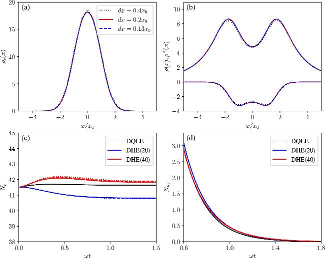
Figure 1. (a), (b) Spatial distributions of the initial state near the trap center for different spatial discretization dx; (c), (d) time evolution of the condensed and non-condensed particle numbers simulated by the DQLE, DHE(20), and DHE(40) schemes with different time step sizes dt. The dot–dashed, dashed, and solid lines correspond to dt = 0.0001, 0.000 07, 0.000 05ω−1, respectively. Results of the three methods are distinguished by color. The system is initialized in equilibrium with parameters g0/ℏωx0 = 0.117 and kbT/ℏω = 16, and then suddenly quenched to g = 0.5g0, with the dissipation rate fixed at γ = 5ω. |
Both the DQLE and DHE dynamics are simulated using a discretized time-evolution scheme. Unlike the case for the Gross–Pitaevskii equation—where spatial derivatives can be handled spectrally via the fast Fourier transform [52]—the presence of strongly coupled equations in our formalism necessitates the use of a fourth-order Runge–Kutta integrator. The details of this standard method can be found in [53]. Numerical convergence with respect to both temporal and spatial discretization has been verified independently. In our simulations, the spatial grid spacing dx varies between 0.13x0 and 0.4 x0 and the time step dt ranges from 0.0001 ω−1 to 0.000 05 ω−1. We find that both the DQLE and DHE results converge as dx and dt are decreased, with dx = 0.2 x0 and dt = 0.000 05 ω−1 yielding a well-converged outcome. Representative convergence tests for both DQLE and DHE are presented in figures 1(c)–(d). We emphasize that all data presented here have been checked for convergence in both space and time.
We also note that the DHE method exhibits greater sensitivity to the smoothness of the input data, requiring a higher density of spatial grid points for stable evolution. To mitigate this, we implement a numerical smoothing procedure that enhances the continuity of discrete spatial derivatives.
4.1. Quench dynamics analysis across different DHE schemes
Before detailing our simulations, we establish criteria for evaluating the various approximations. The comparison is based on key hydrodynamic quantities such as ∣Φ∣2, ρ, jx, ρA, and others. The comparison is based on the absolute deviation between different values as well as some global features of the solutions. The first one can be easily quantified, but the latter could only be displayed by the dynamical evolution. Therefore we will first show the dynamical evolution and then we quantify the variance by absolute deviations.
The particle exchange between the condensate and the normal fluid is captured by the term $| {\rho }^{A}| | {\rm{\Phi }}{| }^{2}\sin (2\theta -\kappa )$. Consequently, an accurate description of ∣Φ∣2, ρ, ρA, jx, and $\sin (2\theta -\kappa )$ enables a clear understanding of the coherent loss process—which is the primary goal of this work. Understanding this coherent particle exchange is essential for comprehending and designing the cooling process. Hence, these hydrodynamic quantities play a central role in our analysis. We also present the higher-order expansion coefficients X, Y, and YA, which help clarify the conditions for the validity of DHE.
In figures 2–5, we compare the quench dynamics of hydrodynamic quantities up to the fourth order in the gradient expansion, using different DHE schemes against the full DQLE reference. All the descriptions of anomalous hydrodynamic quantities show the absolute values. The DHE(20) and DHE(40) schemes remain robust across various quench protocols. Although DHE(44) achieves higher accuracy at very short times, the anomalous density ∣ρA(x, t)∣ grows substantially beyond a characteristic explosion time ${t}_{{\rm{\exp }}}$. As shown in figure 2, significant deviations appear in quantities such as τ and ∣ρA∣. Moreover, while higher-order hydrodynamic coefficients like τA and YA decay rapidly in the full DQLE simulation, their decay is much slower when higher-order terms are retained in the hydrodynamic expansion. This behavior is consistent across different initial conditions and dynamical settings.
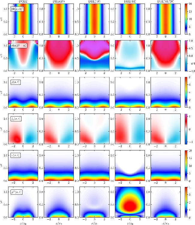
Figure 2. All panels use a fixed dissipation rate γ = 5ω. All the figures are displaying the hydrodynamical quantities for different methods. The system is initialized in equilibrium with parameters g0/ℏωx0 = 0.117 and kbT/ℏω = 16, and then suddenly quenched to g = 0.5g0. The first column shows results from the DQLE model: condensate density ∣Φ(x, t)∣2, phase difference $\sin (2\theta -\kappa )$, normal density ρ(x, t), current jx(x, t), stress tensor τ(x, t), and anomalous density ∣ρA(x, t)∣. Columns 2–4 correspond, respectively, to the DHE(20), DHE(40), and DHE(44) schemes, while column 5 shows results for the DHE(44/20) scheme. One can see there is an ‘explosion' in DHE(44) at a special time. The t0 is designed based on this exploding time. |
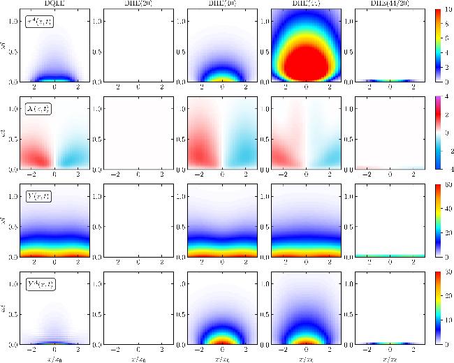
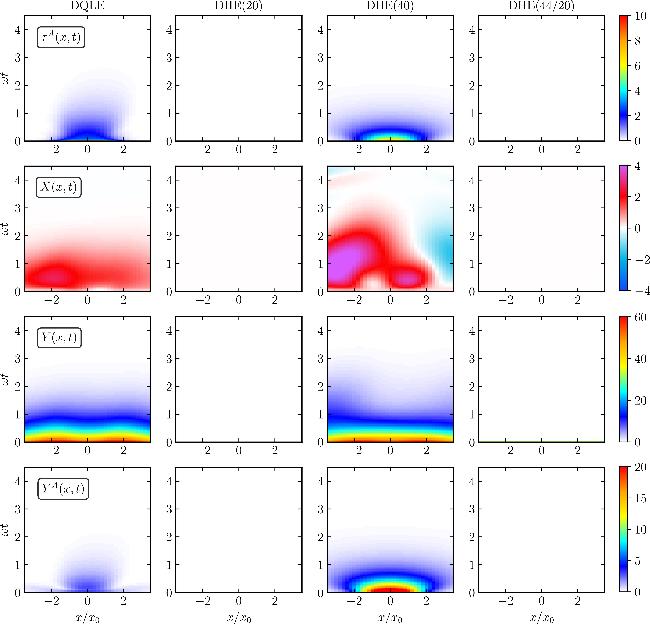
Figure 3. The system is initialized in equilibrium with parameters g0/ℏωx0 = 0.117 and kbT/ℏω = 16, and then suddenly quenched to g = 0.5g0. In different rows, we show anomalous stress tensor ∣τA(x, t)∣, normal hydrodynamical expansion coefficients X(x, t) (third order) and Y(x, t) (fourth order), and the fourth order anomalous coefficient ∣YA(x, t)∣. The first column is DQLE result, the comparison is made in the second to fourth columns for DHE results. Note that these four hydrodynamic quantities do not exist for DHE(20). One can observe that, the τA and YA decays faster than the previous given terms like τ and ρA. Obvious error happens in DHE(44) for these high-order expansion terms. |
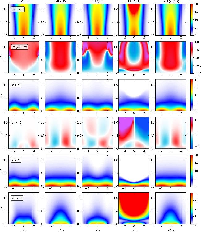
Figure 4. A quench to g = 1.5g0 is performed, with all other parameters matching those in figure 2. All leading order of hydrodynamical expansion coefficients are compared for DQLE and DHE schemes. A clear exploding time is presented in DHE(44) for ρA(x, t). DHE(20) and DHE(44/20) are equally good. |
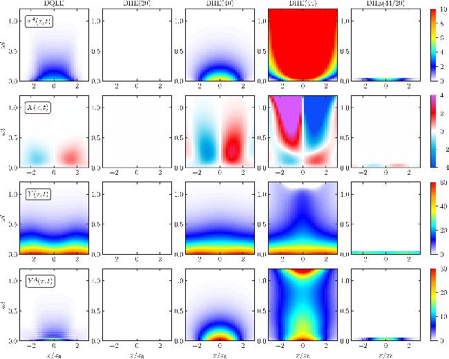
Figure 5. A quench to g = 1.5g0 is performed, with all other parameters matching those in figure 4. We can observe a fast decay in τA and YA. This implies DHE(20) or DHE(40) may be good approximations. |
Thus, although higher-order DHE(MN) schemes with larger M and N improve early-time accuracy, they eventually induce numerical instabilities. This indicates that, despite the rapid decay of high-order hydrodynamic coefficients under dissipation, the full dynamics inherently involve couplings across all orders. While the underlying mechanism is nontrivial, the practical implication is clear: one may either increase the expansion orders M and N, or set N = 0 from the outset. Since the former leads inevitably to instability, we adopt a hybrid approach: we switch from DHE(44) to DHE(20) after a time t0, which we choose as ${t}_{0}={t}_{{\rm{\exp }}}/2.4$ based on the observed explosion time of ρA in the pure DHE(44) scheme. Representative simulations comparing DHE(40) and the hybrid DHE(44/20) method are presented in figures 2–5. One can find in the displaying examples, the hydrodynamical approaches are in general good. The best approximation is DHE(40). It implies that the DHE(60), DHE(80) may serve as better approximations. Even if the theory becomes more complicated, the calculation complexity is greatly removed by hydrodynamical methods.
To evaluate the quantitative accuracy of the DHE schemes, we analyzed the deviation between the DHE and DQLE results for the observable ${ \mathcal W }$. The time-dependent discrepancy is defined as:
$\begin{eqnarray}{\sigma }_{{ \mathcal W }}(t)=\frac{| {{ \mathcal W }}_{{\rm{DHE}}}(t)-{{ \mathcal W }}_{{\rm{DQLE}}}(t)| }{{N}_{{\rm{tot}}}},\end{eqnarray}$
where Ntot is the total number of particles. The analysis focused on key observables, specifically the particle numbers in the condensed (Nc) and non-condensed (Nnc) phases.Here we are discussing the hybrid DHE(44/20) scheme, with the primary objective of determining the optimal switching time t0. To rigorously quantify the accuracy of our approach across this parameter space, we evaluated the dynamical evolution of a key physical observable: the condensed particle number Nc. The results obtained from the DHE(44/20) method were benchmarked against those from the highly accurate DQLE approach, serving as our numerical benchmark. The deviation between these two sets of results ${\sigma }_{{N}_{{\rm{c}}}}(t)$ was meticulously computed and served as our primary metric for precision. A general procedure is introduced to select t0 without prior knowledge of the full DQLE evolution. Specifically, we compute both the DHE(20) and DHE(44) solutions and define the switching time in relation to the explosion time ${t}_{{\rm{\exp }}}$ of the DHE(44) scheme, which is determined by comparing the two hydrodynamic approximations. The detailed informations are included in figure 6.
The time-dependent deviation between DHE and DQLE results for both condensed and non-condensed particle populations is displayed in figures 7 and 8 for different quench protocols with fixed dissipation rates. The system is initiated in a thermal state for g0 = 0.117ℏωx0. The dissipation γ is turned on at time zero. Then we quench the interaction g to a different value than g0 for fixed decay rate γ = 2.5ω and γ = 5ω. In figure 7, we show the deviation for condensed particle number. In figure 8, we show the deviation in dynamics for normal phase particle number. In general, the hydrodynamic approximation performs more accurately under stronger dissipation. Conversely, its validity is progressively reduced for larger interaction quenches. From the comparison, we find a general tendency for enhancement of precision and stability at larger dissipation rate and smaller interaction quench. One can also observe that DHE(40) is the best approximation, which may imply a larger parameter range for the hydrodynamical method to be stable. As we find the dissipation being a key for hydrodynamical method, it is natural that the hydrodynamical method is dropped because of its instability with no external dissipations (previous study set up).
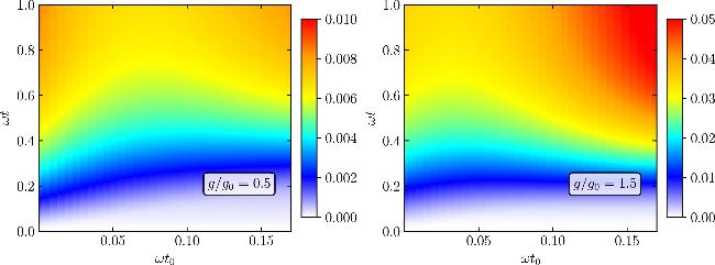
Figure 6. Time evolution of ${\sigma }_{{N}_{{\rm{c}}}}(t)$ for different quench protocols, varying the switching time t0. Initial state and dissipation rate are identical to figure 2. |
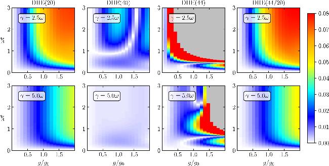
Figure 7. Time evolution of deviation of condensed particle number ${\sigma }_{{N}_{{\rm{c}}}}(t)$ for different quench protocols and dissipation rates across four DHE schemes. The first row corresponds to a dissipation rate of γ = 2.5ω, while the second row corresponds to γ = 5ω. In both rows, the interaction quench parameter g/g0 ranges from 0 to 2. The evolution time is from ωt = 0 to ωt = 3. |
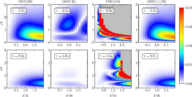
Figure 8. Time evolution of deviation of normal phase particle number ${\sigma }_{{N}_{{\rm{n}}{\rm{c}}}}(t)$ for different quench protocols and dissipation rates across four DHE schemes. All the parameter settings are the same as those in figure 7. |
We also compare DQLE and DHE methods for fixed interaction quench and different dissipation rate protocols in figures 9 and 10. Here the interaction quench is done for g/g0 = 0.5 and 1.5. The dissipation rate is ranging from γ = 2ω to γ = 6ω. The four columns are showing ${\sigma }_{{N}_{{\rm{c}}}}(t)$ (deviation of condensed particle number) and ${\sigma }_{{N}_{{\rm{n}}{\rm{c}}}}(t)$ (deviation of normal phase particle number) for four different DHE approximations. Again the best results are reached in DHE(40). DHE(20) and DHE(44/20) are similar.
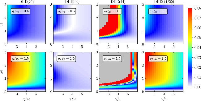
Figure 9. Time evolution of deviation of condened particle number ${\sigma }_{{N}_{{\rm{c}}}}(t)$ for different quench protocols and dissipation rates across four DHE schemes. The first row corresponds to the interaction quench parameter g/g0 = 0.5, while the second row corresponds to g/g0 = 1.5. In both rows, the dissipation rate γ/ω ranges from 2 to 6. The evolution time is from ωt = 0 to ωt = 3. |
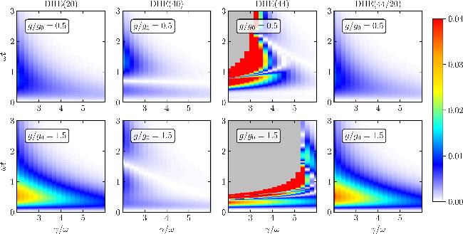
Figure 10. Time evolution of deviation of normal phase particle number ${\sigma }_{{N}_{{\rm{n}}{\rm{c}}}}(t)$ for different quench protocols and dissipation rates across four DHE schemes. All the parameter settings are the same as those in figure 9. |
4.2. Trap center shift dynamics analysis across different DHE schemes
ITo further examine the stability and applicability of the DHE method, we analyze the dipolar oscillation of the condensate following a sudden shift of the trapping potential. This dynamical scenario also involves the evaporation of normal-state particles, providing a stringent test for the numerical schemes. The initial state is prepared identically to the procedure described in the previous analysis (g0 = 0.117ℏωx0 and kbT = 16ℏω). At time t = 0, the harmonic trap center is instantaneously shifted to excite the dipole mode. Specifically, the potential minimum is moved from its initial position at x = 0 to a new center at x = 0.5x0. We then monitor the subsequent evolution, with particular focus on the oscillations of the condensate and the evaporation dynamics of the normal-state particles.
IIn figures 11 and 12, we compare the dynamics of hydrodynamic quantities up to the fourth order in the gradient expansion, evaluating the performance of different DHE schemes against the full DQLE reference. All displayed anomalous hydrodynamic quantities are shown in absolute value. Consistent with earlier analyzes, the results demonstrate that the DHE(20) and DHE(44/20) schemes yield nearly identical dynamical profiles, both capturing the essential trends but with observable deviations from the DQLE baseline in finer details. In contrast, the DHE(40) scheme has the highest degree of conformity with the DQLE reference standard. One may observe that for high-order expansion coefficients of ρA, the decay is still slower than the DQLE case. It shows a possibility for higher accuracy by adding expansion order in normal fluid density matrix. This hierarchy in accuracy underscores the importance of retaining higher-order gradient terms in the expansion when resolving subtle, non-equilibrium hydrodynamic features.
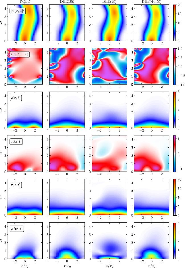
Figure 11. All panels use a fixed dissipation rate γ = 2ω. The first column shows results from the DQLE model: condensate density ∣Φ(x, t)∣2, phase difference $\sin (2\theta -\kappa )$, normal density ρ(x, t), current jx(x, t), stress tensor τ(x, t), and anomalous density ∣ρA(x, t)∣. The system is initialized in equilibrium with parameters g0/ℏωx0 = 0.117 and kbT/ℏω = 16, and then suddenly shifts the center of the trap by 0.5x0. Columns 2–4 correspond, respectively, to the DHE(20), DHE(40), and DHE(44/20) schemes. |
Figure 12. All panels use a fixed dissipation rate γ = 2ω. The system is initialized in equilibrium with parameters g0/ℏωx0 = 0.117 and kbT/ℏω = 16, and then suddenly shifts the center of the trap by 0.5x0. In different rows, we show anomalous stress tensor ∣τA(x, t)∣, normal hydrodynamical expansion coefficients X(x, t) (third order) and Y(x, t) (fourth order), and the fourth order anomalous coefficient ∣YA(x, t)∣. The first column is DQLE result, the comparison is made in the 2–4 columns for DHE results. Note that these four hydrodynamic quantities do not exist for DHE(20). One can observe that, the τA and YA decays faster than the previous given terms like τ and ρA. |
5. Conclusions and discussions
In this work we develop a dissipative quantum Liouville framework for a FT superfluid, from which a systematic hydrodynamic expansion is derived. Our analysis demonstrates that external dissipation serves to both simplify the treatment of inherent damping mechanisms and stabilize the resulting hydrodynamic equations. Through a detailed comparison between the DQLE and various orders of the dissipative hydrodynamic expansion, two principal results emerge. First, early-time accuracy can be systematically improved by increasing the hydrodynamic expansion order, though a characteristic timescale t0 exists beyond which higher-order descriptions deviate significantly. Second, by dropping the high-order hydrodynamical expansion in anomalous density matrix, the dissipative hydrodynamical equations reach a best approximation compared with the DQLE result. By comparing the DHE(20) approximation with DHE(40) approximation, we can expect adding hydrodynamical expansion order in normal fluid density matrix will get better result. Our findings provide a step toward a more first-principles hydrodynamic theory for open quantum many-body systems. Furthermore, they offer a constructive approach for achieving accurate and stable reduced descriptions in the simulation of dissipative quantum dynamics.