Welcome to visit Communications in Theoretical Physics,
Quantum Physics and Quantum Information

Quantifying magic via quantum (αβ) Jensen–Shannon divergence

  • Linmao Wang ,
  • Zhaoqi Wu , *
Expand
  • Department of Mathematics, Nanchang University, Nanchang 330031, China

*Author to whom any correspondence should be addressed.

Received date: 2025-11-29

  Revised date: 2026-02-03

  Accepted date: 2026-02-04

  Online published: 2026-03-04

Copyright

© 2026 Institute of Theoretical Physics CAS, Chinese Physical Society and IOP Publishing. All rights, including for text and data mining, AI training, and similar technologies, are reserved.
This article is available under the terms of the IOP-Standard License.

Abstract

Magic states play an important role in fault-tolerant quantum computation, and so the quantification of magic for quantum states is of great significance. In this work, we propose two new magic quantifiers by introducing two versions of quantum (αβ) Jensen–Shannon divergence, based on the quantum (αβ) entropy and the quantum (αβ)-relative entropy, respectively. We derive many desirable properties for our magic quantifiers, and find that they are efficiently computable in low-dimensional Hilbert spaces. We also show that the initial nonstabilizerness of the input state can boost the magic-generating power for our magic quantifiers with appropriate parameter ranges for a certain class of quantum gates. Our magic quantifiers may provide new tools for addressing some specific problems in magic resource theory.

Cite this article

Linmao Wang , Zhaoqi Wu . Quantifying magic via quantum (αβ) Jensen–Shannon divergence[J]. Communications in Theoretical Physics, 2026 , 78(5) : 055103 . DOI: 10.1088/1572-9494/ae418d

1. Introduction

The Gottesman–Knill theorem indicates that classical computers can efficiently simulate any quantum computation composed solely of Clifford gates and preparation/measurement of stabilizer states [14]. Nonstabilizerness, therefore, plays a crucial role in demonstrating quantum advantage. Veitch et al first introduced the stabilizer resource theory in quantum computation and proposed two magic monotones which are widely employed now [5, 6]. At the same time, several applications of magic resource theory have been extensively studied, such as magic state distillation [713], which has already been studied in entanglement theory [1419].
In the past decades, magic resource theory has rapidly developed. Many quantifiers of magic of quantum states, for instance, the relative entropy of magic and the mana [5], the robustness of magic [20, 21], min-relative entropy and max-relative entropy of magic [22], the thauma [13], stabilizer rank [23], stabilizer extent [24], the stabilizer Rényi entropy [25, 26] and the Lp-norm magic [27, 28], have been proposed, each of which has its own merits. In addition, the quantification of magic for quantum channels has attracted much attention in recent years. Wang et al [13] first introduced the thauma of quantum states and then applied the same idea to propose the thauma of quantum channels [29]. Saxena and Gour [30] studied the magic resource of multi-qubit quantum channels via the generalized robustness and the min-relative entropy. Seddon and Campbell [31] presented channel robustness and magic capacity in n-qubit systems. Recently, Li and Luo [32] employed the channel-state duality and L1-norm magic [28] to propose a new magic quantifier of channel, which is well-defined in all dimensions.
Quantum entropy and quantum divergence are foundational concepts with pervasive applications in resource theory. The concept of generalized quantum entropy was introduced in [33], while the unified $\left(\alpha ,\beta \right)$-relative entropy was proposed in [34], which has been applied to induce resource monotones in different resource theories such as coherence [35] and imaginarity [36]. The uncertainty relations for unified $\left(\alpha ,\beta \right)$-relative entropy of coherence have also been investigated extensively [35, 37]. The quantum Jensen–Shannon divergence was originated in [38], and it has been proved that the square root of the quantum Jensen–Shannon divergence is a true metric on the quantum state space [39]. Moreover, the quantum Jensen–Shannon divergence can naturally yield monotones to quantify magic [40] and imaginarity [41]. In this work, we utilize the quantum (αβ) entropy and the quantum $\left(\alpha ,\beta \right)$-relative entropy to define two versions of quantum (αβ) Jensen–Shannon divergence, and further propose the magic monotones induced by them.
In magic resource theory, a natural question arises as to how we can quantify the power of a quantum gate for generating magic resource. Zhu et al [42] studied amortized magic in terms of the stabilizer Rényi entropy, and revealed that magic generating power can be enhanced by prior nonstabilizerness of input states while considering the α-stabilizer Rényi entropy but this does not hold for the case of robustness of magic [21] or stabilizer extent [24]. When we focus on which quantum gate is optimal for generating magic resource, the answer provided by numerous studies is the T-gate, according to various magic quantifiers under certain conditions [40, 4345].
The remainder of this work is structured as follows. In section 2, we present a brief review of the stabilizer formalism and the framework of magic resource theory. In section 3, we define quantum (αβ) Jensen–Shannon divergence from two distinct ways and derive some properties of them. Specifically, we exhibit a relationship between them, from which a similar relationship between the corresponding magic quantifiers in section 4 follows. In section 4, we define two magic quantifiers via quantum (αβ) Jensen–Shannon divergence and prove that our magic quantifiers are both pure-state stabilizer monotones. Besides, we obtain a few desirable properties and compare our magic quantifiers with the robustness of magic. In section 5, we show that as in the case of the stabilizer Rényi entropy, the magic generating power can also be enhanced by prior magic of input states when considering quantum (αβ) Jensen–Shannon divergence of magic. In section 6, we give three detailed examples. Finally, we conclude our work with a summary in section 7. The detailed proofs of our results are provided in the Appendix.

2. Preliminaries

In this section, we review the stabilizer formalism, the framework of magic resource theory and some basic properties of the quantum (αβ) entropy and the quantum $\left(\alpha ,\beta \right)$-relative entropy.
Let us first clarify some notations which we will use in this paper. Let ${ \mathcal H }$ be a d-dimensional Hilbert space with standard computational basis ${\left\{| i\rangle \right\}}_{i=0}^{d-1}$ and ${{ \mathcal H }}_{{d}^{n}}$ denotes the composite Hilbert space ${{ \mathcal H }}^{\otimes n}$. Denote the set of all density operators by ${ \mathcal D }({ \mathcal H })$, the set of all unitary operators by ${ \mathcal U }({ \mathcal H })$, and the set of all stabilizer states and pure stabilizer states on ${ \mathcal H }$ by ${{ \mathcal S }}_{d}$ and ${ \mathcal P }{{ \mathcal S }}_{d}$, respectively. We conventionally use ρστ to represent quantum states and $| \psi \rangle ,| \psi ^{\prime} \rangle ,| \phi \rangle $ to represent pure states in ${ \mathcal D }({ \mathcal H })$. Moreover, ∥ · ∥1 denotes the trace distance, i.e. $\parallel \rho -\sigma {\parallel }_{1}=\frac{1}{2}{\rm{Tr}}| \rho -\sigma | $.

2.1. Stabilizer formalism

Let ${{\mathbb{Z}}}_{d}$ be the ring of integers modulo d and ${{\mathbb{Z}}}_{d}\times {{\mathbb{Z}}}_{d}$ be the direct product of ${{\mathbb{Z}}}_{d}$ and ${{\mathbb{Z}}}_{d}$ which can be regarded as the discrete phase space. The shift and boost operators are defined as [46]
$\begin{eqnarray*}\begin{array}{r}X=\displaystyle \sum _{j=0}^{d-1}| j+1\rangle \langle j| ,Z=\displaystyle \sum _{j=0}^{d-1}{\omega }^{j}| j\rangle \langle j| ,\end{array}\end{eqnarray*}$
respectively, where $\omega ={\,\rm{e}\,}^{\frac{2\pi {\rm{i}}}{d}}$. And the discrete Heisenberg-Weyl operators are defined as [47]
$\begin{eqnarray*}\begin{array}{r}{T}_{u}={\tau }^{-{u}_{1}{u}_{2}}{Z}^{{u}_{1}}{X}^{{u}_{2}},\end{array}\end{eqnarray*}$
where $\tau ={\,\rm{e}\,}^{\frac{(d+1)\pi {\rm{i}}}{d}},u=({u}_{1},{u}_{2})\in {{\mathbb{Z}}}_{d}\times {{\mathbb{Z}}}_{d}$.
The Clifford operators constitute the set defined as [5]
$\begin{eqnarray*}\begin{array}{rcl}{{ \mathcal C }}_{d} & = & \left\{U\in { \mathcal U }({ \mathcal H }):\forall u\in {{\mathbb{Z}}}_{d}\times {{\mathbb{Z}}}_{d},\exists u^{\prime} \in {{\mathbb{Z}}}_{d}\times {{\mathbb{Z}}}_{d},\right.\\ & & \left.\theta \in {\mathbb{R}},\,{\rm{s.t.}}\,U{T}_{u}{U}^{\dagger }={\,\rm{e}\,}^{{\rm{i}}\theta }{T}_{u^{\prime} }\right\},\end{array}\end{eqnarray*}$
and the set of all pure stabilizer states is defined as [5]
$\begin{eqnarray*}\begin{array}{r}{ \mathcal P }{{ \mathcal S }}_{d}=\left\{V| 0\rangle :V\in {{ \mathcal C }}_{d}\right\},\end{array}\end{eqnarray*}$
while the set of all stabilizer states is the convex hull of ${ \mathcal P }{{ \mathcal S }}_{d}$, i.e. [5],
$\begin{eqnarray*}\begin{array}{rcl}{{ \mathcal S }}_{d} & = & \left\{\rho \in { \mathcal D }({ \mathcal H }):\rho =\displaystyle \sum _{j}{p}_{j}{\rho }_{j},{\left\{{\rho }_{j}\right\}}_{j}\in { \mathcal P }{{ \mathcal S }}_{d},\right.\\ & & \left.{p}_{j}\geqslant 0,\displaystyle \sum _{j}{p}_{j}=1\right\}.\end{array}\end{eqnarray*}$
A quantum state is a magic state if it is not a stabilizer state.
A stabilizer operation is any map from $\rho \in { \mathcal D }\left({{ \mathcal H }}_{{d}^{n}}\right)$ to $\sigma \in { \mathcal D }\left({{ \mathcal H }}_{{d}^{m}}\right)$ composed from the following operations [5]
(i) Clifford unitaries, ρ → VρV where $V\in {{ \mathcal C }}_{d}$.
(ii) Composition with stabilizer states, ρ → ρ ⨂ σ where $\sigma \in {{ \mathcal S }}_{d}$.
(iii) Computational basis measurement on the final qudit, $\rho \to \frac{\left({\mathbb{I}}\otimes | i\rangle \langle i| \right)\rho \left({\mathbb{I}}\otimes | i\rangle \langle i| \right)}{\,\rm{Tr}\,\left(\rho {\mathbb{I}}\otimes | i\rangle \langle i| \right)}$ with probability ${\rm{Tr}}\,\left(\rho {\mathbb{I}}\otimes | i\rangle \langle i| \right)$, where ${\mathbb{I}}$ is the identity operator on ${ \mathcal D }\left({{ \mathcal H }}_{{d}^{n-1}}\right)$.
(iv) Partial trace of the final qudit, $\rho \to {\,\rm{Tr}\,}_{n}\left(\rho \right)$.
(v) The above quantum operations conditioned on the outcomes of measurements or classical randomness.

2.2. The framework of magic resource theory

Two important ingredients of a resource theory are free states and free operations. In magic resource theory, free states and free operations refer to stabilizer states and stabilizer operations. We first recall the framework of the quantification of magic resource for quantum states.
A functional ${ \mathcal M }$ that maps ${ \mathcal D }({ \mathcal H })$ to [0, + ) is called a magic measure if it satisfies [48]
(i) Faithfulness: ${ \mathcal M }(\rho )=0$ if and only if $\rho \in {{ \mathcal S }}_{d}$.
(ii) Monotonicity: ${ \mathcal M }({ \mathcal E }(\rho ))\leqslant { \mathcal M }(\rho )$ for any stabilizer operation ${ \mathcal E }$.
(iii) Convexity: ${ \mathcal M }({\sum }_{j}{p}_{j}{\rho }_{j})\leqslant {\sum }_{j}{p}_{j}{ \mathcal M }({\rho }_{j})$ for any ${\left\{{\rho }_{j}\right\}}_{j}\in { \mathcal D }({ \mathcal H })$ and probability distribution ${\left\{{p}_{j}\right\}}_{j}$.
(iv) Strong monotonicity: ${ \mathcal M }(\rho )\geqslant {\sum }_{j}{p}_{j}{ \mathcal M }({\rho }_{j})$ for any stabilizer operation ${ \mathcal E }$ satisfying ${ \mathcal E }(\rho )={\sum }_{j}{p}_{j}{\rho }_{j}$.
If ${ \mathcal M }$(·) only satisfies properties (i) and (ii), we say that ${ \mathcal M }$(·) is a magic monotone. And ${ \mathcal M }$(·) is called a pure-state stabilizer monotone if it satisfies [26]
${({\rm{i}})}^{{\prime} }$ Faithfulness: ${ \mathcal M }(| \psi \rangle \langle \psi | )=0$ if and only if $| \psi \rangle \in { \mathcal P }{{ \mathcal S }}_{d}$.
${({\rm{ii}})}^{{\prime} }$ Monotonicity: ${ \mathcal M }(| \phi \rangle \langle \phi | )\leqslant { \mathcal M }(| \psi \rangle \langle \psi | )$ for any stabilizer operation ${ \mathcal E }$ satisfying ${ \mathcal E }(| \psi \rangle \langle \psi | )=| \phi \rangle \langle \phi | $.
A good magic quantifier should be at least a pure-state stabilizer monotone.

2.3. The quantum (αβ) entropy and the quantum $\left(\alpha ,\beta \right)$-relative entropy

The quantum (αβ) entropy is defined as [33]
$\begin{eqnarray*}\begin{array}{r}\begin{array}{l}{S}_{\alpha ,\beta }\left(\rho \right)=\frac{1}{(1-\alpha )\beta }\left[{\left({\rm{Tr}}({\rho }^{\alpha })\right)}^{\beta }-1\right],\\ \,\,\alpha \in (0,1)\cup (1,+\infty ),\\ \,\,\beta \in (-\infty ,0)\cup (0,+\infty ),\end{array}\end{array}\end{eqnarray*}$
and the quantum $\left(\alpha ,\beta \right)$-relative entropy is defined as [34]
$\begin{eqnarray*}\begin{array}{r}\begin{array}{l}{D}_{\alpha ,\beta }\left(\rho \parallel \sigma \right)=\frac{1}{(1-\alpha )\beta }\left[1-{\left({\rm{Tr}}\left({\rho }^{\alpha }{\sigma }^{1-\alpha }\right)\right)}^{\beta }\right],\\ \alpha \in (0,1)\cup (1,+\infty ),\\ \beta \in (-\infty ,0)\cup (0,+\infty ).\end{array}\end{array}\end{eqnarray*}$
Throughout this paper, we follow the convention that for any density operator $\rho \in { \mathcal D }({ \mathcal H })$, ρ−1 is only evaluated on its support, i.e. we retain the zero eigenvalues of ρ−1, thus it is reasonable to define Dα,β(ρσ) for α ∈ (1, + ).
The basic properties of Sα,β(ρ) and ${D}_{\alpha ,\beta }\left(\rho \parallel \sigma \right)$ are summarized in the following two lemmas, which will be useful in the next section.
([<a href="javascript:;" class="mag_content_a" onclick="piaofuRef(this,'ctpae418dbib33')" rid="ctpae418dbib33">33</a>, <a href="javascript:;" class="mag_content_a" onclick="piaofuRef(this,'ctpae418dbib49')" rid="ctpae418dbib49">49</a>])

Let ${\left\{{\rho }_{j}\right\}}_{j}\in { \mathcal D }({ \mathcal H })$, and ${\left\{{p}_{j}\right\}}_{j}$ be a probability distribution. Then we have

(i) (Concavity) For α ∈ (0, 1), β ∈ ( − , 0) ∪ (0, 1], it holds that

$\begin{eqnarray*}\begin{array}{r}{S}_{\alpha ,\beta }\left(\displaystyle \sum _{j}^{}{p}_{j}{\rho }_{j}\right)\geqslant \displaystyle \sum _{j}^{}{p}_{j}{S}_{\alpha ,\beta }\left({\rho }_{j}\right),\end{array}\end{eqnarray*}$
and for α ∈ (1, + ), β ∈ [1, + ), it holds that
$\begin{eqnarray*}\begin{array}{rcl}\displaystyle \sum _{j}^{}{p}_{j}{S}_{\alpha ,\beta }({\rho }_{j}) & \leqslant & {S}_{\alpha ,\beta }\left(\displaystyle \sum _{j}^{}{p}_{j}{\rho }_{j}\right)\\ & \leqslant & \displaystyle \sum _{j}^{}{p}_{j}{S}_{\alpha ,\beta }\left({\rho }_{j}\right)+{F}_{\alpha }^{\beta }\left({\left\{{p}_{j}\right\}}_{j}\right),\end{array}\end{eqnarray*}$
where
$\begin{eqnarray*}\begin{array}{r}{F}_{\alpha }^{\beta }\left({\left\{{p}_{j}\right\}}_{j}\right)=\frac{1}{(1-\alpha )\beta }\left(\displaystyle \sum _{j}^{}{p}_{j}^{\alpha \beta }-1\right).\end{array}\end{eqnarray*}$

(ii) For α ∈ (0, 1) ∪ (1, +), β ∈ (−, 0) ∪ (0, +), it holds that

$\begin{eqnarray*}\begin{array}{rcl}{S}_{\alpha ,\beta }\left(\rho \displaystyle \otimes \sigma \right) & = & {S}_{\alpha ,\beta }\left(\rho \right)+{S}_{\alpha ,\beta }\left(\sigma \right)\\ & & +(1-\alpha )\beta {S}_{\alpha ,\beta }\left(\rho \right){S}_{\alpha ,\beta }\left(\sigma \right).\end{array}\end{eqnarray*}$

(iii) (Unitary invariance) For α ∈ (0, 1) ∪ (1, +), β ∈ (−, 0) ∪ (0, +) and any unitary operator $U\in { \mathcal U }({ \mathcal H })$, it holds that

$\begin{eqnarray*}\begin{array}{r}{S}_{\alpha ,\beta }\left(\rho \right)={S}_{\alpha ,\beta }\left(U\rho {U}^{\dagger }\right).\end{array}\end{eqnarray*}$

(iv) (Lipschitz continuity) For α ∈ (1, +), β ∈ [1, +), it holds that

$\begin{eqnarray*}\begin{array}{r}| {S}_{\alpha ,\beta }(\rho )-{S}_{\alpha ,\beta }(\sigma )| \leqslant \frac{\alpha }{\alpha -1}\parallel \rho -\sigma {\parallel }_{1}.\end{array}\end{eqnarray*}$

([<a href="javascript:;" class="mag_content_a" onclick="piaofuRef(this,'ctpae418dbib34')" rid="ctpae418dbib34">34</a>])

Let ${\left\{{\rho }_{j}\right\}}_{j},{\left\{{\sigma }_{j}\right\}}_{j}\in { \mathcal D }({ \mathcal H })$, and ${\left\{{p}_{j}\right\}}_{j}$ be a probability distribution. Then we have

(i) For α ∈ (0, 1) ∪ (1, +), β ∈ (−, 0) ∪ (0, +), it holds that

$\begin{eqnarray*}\begin{array}{r}{D}_{\alpha ,\beta }\left(\rho \parallel \sigma \right)\geqslant 0,\end{array}\end{eqnarray*}$
and the equality holds if and only if ρ = σ.

(ii) For α ∈ (0, 1) ∪ (1, +), β ∈ (−, 0) ∪ (0, +), it holds that

$\begin{eqnarray*}\begin{array}{l}{D}_{\alpha ,\beta }\left({\rho }_{1}\displaystyle \otimes {\rho }_{2}\parallel {\sigma }_{1}\displaystyle \otimes {\sigma }_{2}\right)={D}_{\alpha ,\beta }\left({\rho }_{1}\parallel {\sigma }_{1}\right)+{D}_{\alpha ,\beta }\left({\rho }_{2}\parallel {\sigma }_{2}\right)\\ \quad +(\alpha -1)\beta {D}_{\alpha ,\beta }\left({\rho }_{1}\parallel {\sigma }_{1}\right){D}_{\alpha ,\beta }\left({\rho }_{2}\parallel {\sigma }_{2}\right).\end{array}\end{eqnarray*}$

(iii) (Monotonicity) For any quantum operation ${ \mathcal E }$ and α ∈ (0, 1), β ∈ (−, 0) ∪ (0, 1], it holds that

$\begin{eqnarray*}\begin{array}{r}{D}_{\alpha ,\beta }\left({ \mathcal E }(\rho )\parallel { \mathcal E }(\sigma )\right)\leqslant {D}_{\alpha ,\beta }\left(\rho \parallel \sigma \right).\end{array}\end{eqnarray*}$

(iv) (Unitary invariance) For α ∈ (0, 1) ∪ (1, +), β ∈ (−, 0) ∪ (0, +) and any unitary operator $U\in { \mathcal U }({ \mathcal H })$, it holds that

$\begin{eqnarray*}\begin{array}{r}{D}_{\alpha ,\beta }\left(U\rho {U}^{\dagger }\parallel U\sigma {U}^{\dagger }\right)={D}_{\alpha ,\beta }\left(\rho \parallel \sigma \right).\end{array}\end{eqnarray*}$

(v) (Joint convexity) For α ∈ (0, 1), β ∈ (−, 0) ∪ (0, 1], it holds that

$\begin{eqnarray*}\begin{array}{r}{D}_{\alpha ,\beta }\left(\displaystyle \sum _{j}^{}{p}_{j}{\rho }_{j}\parallel \displaystyle \sum _{j}^{}{p}_{j}{\sigma }_{j}\right)\leqslant \displaystyle \sum _{j}^{}{p}_{j}{D}_{\alpha ,\beta }\left({\rho }_{j},{\sigma }_{j}\right).\end{array}\end{eqnarray*}$

3. Quantum (αβ) Jensen–Shannon divergence

In this section, we present the definition and some properties of the quantum (αβ) Jensen–Shannon divergence.
The quantum Jensen–Shannon divergence is defined as [38]
$\begin{eqnarray*}\begin{array}{rcl}J(\rho ,\sigma ) & = & \frac{1}{2}\left[D\left(\rho \parallel \frac{\rho +\sigma }{2}\right)+D\left(\sigma \parallel \frac{\rho +\sigma }{2}\right)\right]\\ & = & S\left(\frac{\rho +\sigma }{2}\right)-\frac{1}{2}S(\rho )-\frac{1}{2}S(\sigma ),\end{array}\end{eqnarray*}$
where $S(\rho )=-{\rm{Tr}}\rho {\mathrm{log}}\rho $ is the von Neumann entropy of ρ and $D(\rho \parallel \sigma )={\rm{Tr}}(\rho {\mathrm{log}}\rho -\rho {\mathrm{log}}\sigma )$ is the relative entropy between ρ and σ.
Motivated by the above concepts, we now define the quantum (αβ) Jensen–Shannon divergence as follows.

For α ∈ (0, 1) ∪(1, +), β ∈ (−, 0) ∪ (0, +), we define two kinds of quantum (αβ) Jensen–Shannon divergence as

$\begin{eqnarray}{\,J}_{\alpha ,\beta }(\rho ,\sigma )={S}_{\alpha ,\beta }\left(\frac{\rho +\sigma }{2}\right)-\frac{1}{2}{S}_{\alpha ,\beta }\left(\rho \right)-\frac{1}{2}{S}_{\alpha ,\beta }\left(\sigma \right),\end{eqnarray}$
and
$\begin{eqnarray}{J}_{\alpha ,\beta }^{{\prime} }(\rho ,\sigma )=\frac{1}{2}\left[{D}_{\alpha ,\beta }\left(\rho \parallel \frac{\rho +\sigma }{2}\right)+{D}_{\alpha ,\beta }\left(\sigma \parallel \frac{\rho +\sigma }{2}\right)\right].\end{eqnarray}$

Equations (1) and (2) both degenerate to the quantum Jensen–Shannon divergence introduced in [38] when α → 1, since Sα,β(ρ) and Dα,β(ρσ) degenerate to S(ρ) and D(ρσ) respectively when α → 1. Moreover, equations (1) and (2) reduce to two versions of quantum Jensen–Tsallis divergence proposed in [50] when β = 1, which do not coincide.

For any α ∈ (0, 1) ∪ (1, 2), β ∈ (−, 0) ∪(0, +), it holds that

$\begin{eqnarray}{J}_{\alpha ,\beta }\left(| \psi \rangle \langle \psi | ,| \phi \rangle \langle \phi | \right)={J}_{2-\alpha ,\beta }^{{\prime} }\left(| \psi \rangle \langle \psi | ,| \phi \rangle \langle \phi | \right).\end{eqnarray}$

We leave the proof of proposition 1 in appendix A.1.
Based on lemma 1 and lemma 2, the properties of Jα,β(ρσ) and ${J}_{\alpha ,\beta }^{{\prime} }(\rho ,\sigma )$ can be derived as follows.

Let ${\rho }_{1},{\rho }_{2},{\sigma }_{1},{\sigma }_{2}\in { \mathcal D }({ \mathcal H })$, ${\left\{| {\psi }_{j}\rangle \right\}}_{j}$, ${\left\{| {\phi }_{j}\rangle \right\}}_{j}$ are pure states on ${ \mathcal H }$, and ${\left\{{p}_{j}\right\}}_{j}$ is a probability distribution. Then we have

(i) It holds that

$\begin{eqnarray*}\begin{array}{r}{J}_{\alpha ,\beta }(\rho ,\sigma )\geqslant 0\end{array},\end{eqnarray*}$
for α ∈ (0, 1), β ∈ ( − , 0) ∪ (0, 1) or α ∈ (1, + ), β ∈ [1, + ), and
$\begin{eqnarray*}\begin{array}{r}{J}_{\alpha ,\beta }(\rho ,\sigma )\leqslant \frac{1}{(1-\alpha )\beta }\left({2}^{1-\alpha \beta }-1\right)\end{array},\end{eqnarray*}$
for α ∈ (1, +), β ∈ [1, +).

(ii) For α ∈ (0, 1) ∪ (1, +), β ∈ (−, 0)∪(0, +), it holds that

$\begin{eqnarray*}\begin{array}{r}{J}_{\alpha ,\beta }(\rho \displaystyle \otimes \tau ,\sigma \displaystyle \otimes \tau )=\left[1+(1-\alpha )\beta {S}_{\alpha ,\beta }(\tau )\right]{J}_{\alpha ,\beta }(\rho ,\sigma ).\end{array}\end{eqnarray*}$
Specifically, when τ is a pure state, we have Jα,β(ρ ⨂ τσ ⨂ τ) = Jα,β(ρσ).

(iii) (Unitary invariance) For α ∈ (0, 1) ∪ (1, +), β ∈ (−, 0)∪(0, +) and any unitary operator $U\in { \mathcal U }({ \mathcal H })$, it holds that

$\begin{eqnarray*}\begin{array}{r}{J}_{\alpha ,\beta }(U\rho {U}^{\dagger },U\sigma {U}^{\dagger })={J}_{\alpha ,\beta }(\rho ,\sigma ).\end{array}\end{eqnarray*}$

(iv) (Symmetry) For α ∈ (0, 1) ∪ (1, +), β ∈ ( − , 0)∪(0, +), it holds that

$\begin{eqnarray*}\begin{array}{r}{J}_{\alpha ,\beta }(\rho ,\sigma )={J}_{\alpha ,\beta }(\sigma ,\rho ).\end{array}\end{eqnarray*}$

(v) (Lipschitz continuity) For α ∈ (1, + ), β ∈ [1, + ), Jα,β(ρσ) is Lipschitz continuous in the first or second entry, i.e.

$\begin{eqnarray*}\begin{array}{r}| {J}_{\alpha ,\beta }({\rho }_{1},\sigma )-{J}_{\alpha ,\beta }({\rho }_{2},\sigma )| \leqslant \frac{\alpha }{\alpha -1}\parallel {\rho }_{1}-{\rho }_{2}{\parallel }_{1},\end{array}\end{eqnarray*}$
and
$\begin{eqnarray*}\begin{array}{r}| {J}_{\alpha ,\beta }(\rho ,{\sigma }_{1})-{J}_{\alpha ,\beta }(\rho ,{\sigma }_{2})| \leqslant \frac{\alpha }{\alpha -1}\parallel {\sigma }_{1}-{\sigma }_{2}{\parallel }_{1}.\end{array}\end{eqnarray*}$

We leave the proof of theorem 1 in appendix A.2.

Let ${\left\{{\rho }_{j}\right\}}_{j},{\left\{{\sigma }_{j}\right\}}_{j}\in { \mathcal D }({ \mathcal H })$, and ${\left\{{p}_{j}\right\}}_{j}$ be a probability distribution. Then we have

(i) For α ∈ (0, 1) ∪ (1, + ), β ∈ ( − , 0) ∪ (0, + ), it holds that

$\begin{eqnarray*}\begin{array}{r}{J}_{\alpha ,\beta }^{{\prime} }(\rho ,\sigma )\geqslant 0,\end{array}\end{eqnarray*}$
and the equality holds if and only if ρ = σ.

(ii) For α ∈ (0, 1) ∪ (1, + ), β ∈ ( − , 0)∪(0, + ), it holds that

$\begin{eqnarray*}\begin{array}{r}{J}_{\alpha ,\beta }^{{\prime} }(\rho \displaystyle \otimes \tau ,\sigma \displaystyle \otimes \tau )={J}_{\alpha ,\beta }^{{\prime} }(\rho ,\sigma ).\end{array}\end{eqnarray*}$

(iii) (Monotonicity) For any quantum operation ${ \mathcal E }$ and α ∈ (0, 1), β ∈ ( − , 0) ∪ (0, 1], it holds that

$\begin{eqnarray*}\begin{array}{r}{J}_{\alpha ,\beta }^{{\prime} }\left({ \mathcal E }(\rho ),{ \mathcal E }(\sigma )\right)\leqslant {J}_{\alpha ,\beta }^{{\prime} }(\rho ,\sigma ).\end{array}\end{eqnarray*}$

(iv) (Unitary invariance) For α ∈ (0, 1) ∪ (1, + ), β ∈ ( − , 0)∪(0, + ) and any unitary operator $U\in { \mathcal U }({ \mathcal H })$, it holds that

$\begin{eqnarray*}\begin{array}{r}{J}_{\alpha ,\beta }^{{\prime} }(U\rho {U}^{\dagger },U\sigma {U}^{\dagger })={J}_{\alpha ,\beta }^{{\prime} }(\rho ,\sigma ).\end{array}\end{eqnarray*}$

(v) (Joint convexity) For α ∈ (0, 1), β ∈ ( − , 0) ∪(0, 1], it holds that

$\begin{eqnarray*}\begin{array}{r}{J}_{\alpha ,\beta }^{{\prime} }\left(\displaystyle \sum _{j}^{}{p}_{j}{\rho }_{j},\displaystyle \sum _{j}^{}{p}_{j}{\sigma }_{j}\right)\leqslant \displaystyle \sum _{j}^{}{p}_{j}{J}_{\alpha ,\beta }^{{\prime} }\left({\rho }_{j},{\sigma }_{j}\right).\end{array}\end{eqnarray*}$

(vi) (Symmetry) For α ∈ (0, 1) ∪ (1, ), β ∈ ( − , 0)∪(0, + ), it holds that

$\begin{eqnarray*}\begin{array}{r}{J}_{\alpha ,\beta }^{{\prime} }(\rho ,\sigma )={J}_{\alpha ,\beta }^{{\prime} }(\sigma ,\rho ).\end{array}\end{eqnarray*}$

We leave the proof of theorem 2 in appendix A.3.

By applying proposition 1 and theorem 2(iii), for α ∈ (1, 2), β ∈ ( − , 0) ∪ (0, 1] and any stabilizer operation ${ \mathcal E }$ satisfying ${ \mathcal E }(| \psi \rangle \langle \psi | )=| \psi ^{\prime} \rangle \langle \psi ^{\prime} | $which means that ${ \mathcal E }$ maps a pure state to another pure state, we have

$\begin{eqnarray}{J}_{\alpha ,\beta }\left({ \mathcal E }\left(| \psi \rangle \langle \psi | \right),{ \mathcal E }(| \phi \rangle \langle \phi | )\right)\leqslant {J}_{\alpha ,\beta }\left(| \psi \rangle \langle \psi | ,| \phi \rangle \langle \phi | \right).\end{eqnarray}$

4. Quantum (αβ) Jensen–Shannon divergence of magic

In this section, we present the definition and some properties of the quantum (αβ) Jensen–Shannon divergence of magic, and compare our magic quantifiers with other existing ones.

4.1. Two new stabilizer monotones

We start by defining two magic quantifiers for pure states via the quantum (αβ) Jensen–Shannon divergence.

For α ∈ (0, 1) ∪(1, + ),β ∈ ( − , 0)∪(0, + ), define

$\begin{eqnarray}{M}_{\alpha ,\beta }\left(| \psi \rangle \langle \psi | \right)=\mathop{\min }\limits_{| \phi \rangle \in { \mathcal P }{{ \mathcal S }}_{d}}{J}_{\alpha ,\beta }\left(| \psi \rangle \langle \psi | ,| \phi \rangle \langle \phi | \right),\end{eqnarray}$
$\begin{eqnarray}{m}_{\alpha ,\beta }\left(| \psi \rangle \langle \psi | \right)=\mathop{\min }\limits_{| \phi \rangle \in { \mathcal P }{{ \mathcal S }}_{d}}{J}_{\alpha ,\beta }^{{\prime} }\left(| \psi \rangle \langle \psi | ,| \phi \rangle \langle \phi | \right).\end{eqnarray}$

Next we use convex roof construction to define the quantum (αβ) Jensen–Shannon divergence of magic for mixed states.

For α ∈ (0, 1) ∪ (1, + ), β ∈ ( − , 0)∪(0, + ), we define two kinds of quantum (αβ) Jensen–Shannon divergence of magic as

$\begin{eqnarray}{M}_{\alpha ,\beta }\left(\rho \right)=\mathop{\min }\limits_{\left\{({p}_{j},| {\psi }_{j}\rangle )\right\}}\displaystyle \sum _{j}^{}{p}_{j}{M}_{\alpha ,\beta }\left(| {\psi }_{j}\rangle \langle {\psi }_{j}| \right),\end{eqnarray}$
$\begin{eqnarray}{m}_{\alpha ,\beta }\left(\rho \right)=\mathop{\min }\limits_{\left\{({p}_{j},| {\psi }_{j}\rangle )\right\}}\displaystyle \sum _{j}^{}{p}_{j}{m}_{\alpha ,\beta }\left(| {\psi }_{j}\rangle \langle {\psi }_{j}| \right),\end{eqnarray}$
where $\rho ={\sum }_{j}^{}{p}_{j}| {\psi }_{j}\rangle \langle {\psi }_{j}| $ are all pure-state decompositions of ρ.

From the proof of proposition 1, we can see that
$\begin{eqnarray}{M}_{\alpha ,\beta }\left(| \psi \rangle \langle \psi | \right)=\mathop{\min }\limits_{| \phi \rangle \in { \mathcal P }{{ \mathcal S }}_{d}}\frac{1}{(1-\alpha )\beta }\left[{\left({\lambda }_{1}^{\alpha }+{\lambda }_{2}^{\alpha }\right)}^{\beta }-1\right],\end{eqnarray}$
and
$\begin{eqnarray}{m}_{\alpha ,\beta }\left(| \psi \rangle \langle \psi | \right)=\mathop{\min }\limits_{| \phi \rangle \in { \mathcal P }{{ \mathcal S }}_{d}}\frac{1}{(1-\alpha )\beta }\left[1-{\left({\lambda }_{1}^{2-\alpha }+{\lambda }_{2}^{2-\alpha }\right)}^{\beta }\right],\end{eqnarray}$
where ${\lambda }_{1}=\frac{1+| \langle \psi | \phi \rangle | }{2}$ and ${\lambda }_{2}=\frac{1-| \langle \psi | \phi \rangle | }{2}$ are the eigenvalues of $\frac{| \psi \rangle \langle \psi | +| \phi \rangle \langle \phi | }{2}$. This implies that
$\begin{eqnarray}{m}_{\alpha ,\beta }\left(\rho \right)={M}_{2-\alpha ,\beta }\left(\rho \right),\end{eqnarray}$
for α ∈ (0, 1) ∪ (1, 2), β ∈ ( − , 0) ∪ (0, + ).

Both of the quantities in equations (7) and (8) degenerate to the quantum Jensen–Shannon divergence of magic in [40] when α → 1.

Next we give some properties of ${M}_{\alpha ,\beta }\left(\rho \right)$ and ${m}_{\alpha ,\beta }\left(\rho \right)$.

Let ${\left\{{\rho }_{j}\right\}}_{j}\in { \mathcal D }({ \mathcal H })$, and ${\left\{{p}_{j}\right\}}_{j}$ be a probability distribution. Then we have

(i) (Faithfulness) For α ∈ (0, 1) ∪ (1, + ), β ∈ ( − , 0)∪(0, + ), it holds that

$\begin{eqnarray*}\begin{array}{r}{M}_{\alpha ,\beta }\left(\rho \right)\geqslant 0,\end{array}\end{eqnarray*}$
and the equality holds if and only if $\rho \in {{ \mathcal S }}_{d}$.

(ii) (Invariance under Clifford operations) For any Clifford operator $V\in {{ \mathcal C }}_{d}$ and α ∈ (0, 1) ∪ (1, + ),β ∈ ( − , 0)∪(0, + ), it holds that

$\begin{eqnarray*}\begin{array}{r}{M}_{\alpha ,\beta }\left(V\rho {V}^{\dagger }\right)={M}_{\alpha ,\beta }\left(\rho \right).\end{array}\end{eqnarray*}$

(iii) (Convexity) For α ∈ (0, 1) ∪ (1, + ), β ∈ ( − , 0)∪(0, + ), it holds that

$\begin{eqnarray*}\begin{array}{r}{M}_{\alpha ,\beta }\left(\displaystyle \sum _{j}^{}{p}_{j}{\rho }_{j}\right)\leqslant \displaystyle \sum _{j}^{}{p}_{j}{M}_{\alpha ,\beta }\left({\rho }_{j}\right).\end{array}\end{eqnarray*}$

(iv) (Monotonicity) For α ∈ (1, 2), β ∈ ( − , 0) ∪ (0, 1] and any stabilizer operation ${ \mathcal E }$ which obeys ${ \mathcal E }(| \psi \rangle \langle \psi | )=| \phi \rangle \langle \phi | $, it holds that

$\begin{eqnarray*}\begin{array}{r}{M}_{\alpha ,\beta }\left(| \phi \rangle \langle \phi | \right)\leqslant {M}_{\alpha ,\beta }\left(| \psi \rangle \langle \psi | \right).\end{array}\end{eqnarray*}$

(v) For α ∈ (1, 2), β ∈ ( − , 0) ∪ (0, 1], it holds that

$\begin{eqnarray*}\begin{array}{r}{M}_{\alpha ,\beta }\left(\rho \displaystyle \otimes \sigma \right)\geqslant {M}_{\alpha ,\beta }\left(\rho \right),\end{array}\end{eqnarray*}$
and the equality holds if $\sigma \in {{ \mathcal S }}_{d}$.

(vi) (Lipschitz continuity) For α ∈ (1, + ), β ∈ [1, + ), Mα,β(ρ) is Lipschitz continuous for pure states, i.e.

$\begin{eqnarray*}\begin{array}{r}\begin{array}{l}| {M}_{\alpha ,\beta }(| {\psi }_{1}\rangle \langle {\psi }_{1}| )-{M}_{\alpha ,\beta }(| {\psi }_{2}\rangle \langle {\psi }_{2}| )| \\ \quad \leqslant \frac{\alpha }{\alpha -1}| | | {\psi }_{1}\rangle \langle {\psi }_{1}| -| {\psi }_{2}\rangle \langle {\psi }_{2}| | {| }_{1}.\end{array}\end{array}\end{eqnarray*}$

We leave the proof of theorem 3 in appendix A.4.
By imitating the proof of theorem 3 and utilizing theorem 2, we can also prove that mα,β exhibits the following desirable properties.

Let ${\left\{{\rho }_{j}\right\}}_{j}\in { \mathcal D }({ \mathcal H })$, and ${\left\{{p}_{j}\right\}}_{j}$ be a probability distribution. Then we have

(i) (Faithfulness) For α ∈ (0, 1) ∪ (1, + ),β ∈ ( − , 0)∪(0, + ), it holds that

$\begin{eqnarray*}\begin{array}{r}{m}_{\alpha ,\beta }\left(\rho \right)\geqslant 0,\end{array}\end{eqnarray*}$
and the equality holds if and only if $\rho \in {{ \mathcal S }}_{d}$.

(ii) (Invariance under Clifford operations) For any Clifford operator $V\in {{ \mathcal C }}_{d}$ and α ∈ (0, 1)∪(1, + ),β ∈ ( − , 0)∪(0, + ), it holds that

$\begin{eqnarray*}\begin{array}{r}{m}_{\alpha ,\beta }\left(V\rho {V}^{\dagger }\right)={m}_{\alpha ,\beta }\left(\rho \right).\end{array}\end{eqnarray*}$

(iii) (Convexity) For α ∈ (0, 1) ∪ (1, + ),β ∈ ( − , 0)∪(0, + ) and ρ = ∑jpjρj, convexity holds, i.e.

$\begin{eqnarray*}\begin{array}{r}{m}_{\alpha ,\beta }\left(\displaystyle \sum _{j}^{}{p}_{j}{\rho }_{j}\right)\leqslant \displaystyle \sum _{j}^{}{p}_{j}{m}_{\alpha ,\beta }\left({\rho }_{j}\right).\end{array}\end{eqnarray*}$

(iv) (Monotonicity) For α ∈ (0, 1), β ∈ ( − , 0) ∪ (0, 1] and any stabilizer operation ${ \mathcal E }$ which satisfying ${ \mathcal E }(| \psi \rangle \langle \psi | )=| \phi \rangle \langle \phi | $, it holds that

$\begin{eqnarray*}\begin{array}{r}{m}_{\alpha ,\beta }\left(| \phi \rangle \langle \phi | \right)\leqslant {m}_{\alpha ,\beta }\left(| \psi \rangle \langle \psi | \right).\end{array}\end{eqnarray*}$

(v) For α ∈ (0, 1), β ∈ ( − , 0) ∪ (0, 1], it holds that

$\begin{eqnarray*}\begin{array}{r}{m}_{\alpha ,\beta }\left(\rho \displaystyle \otimes \sigma \right)\geqslant {m}_{\alpha ,\beta }\left(\rho \right),\end{array}\end{eqnarray*}$
and the equality holds if $\sigma \in {{ \mathcal S }}_{d}$.

The above two theorems show that the two versions of quantum (αβ) Jensen–Shannon divergence of magic are both pure-state stabilizer monotones with suitable parameter ranges which will be very helpful while dealing with some pure-state issues. Since Mα,β(ρ) and mα,β(ρ) share similar properties and are closely related, we may only focus on discussing Mα,β(ρ) in the rest of our work.
We first present two obvious lemmas which are easy to verify.

The function

$\begin{eqnarray}g(x,\alpha ,\beta )=\frac{{x}^{\beta }-1}{(1-\alpha )\beta }\end{eqnarray}$
satisfies

(i) g(xαβ) is strictly monotonically increasing for α ∈ (0, 1), β ∈ ( − , 0) ∪ (0, + ) and strictly monotonically decreasing for α ∈ (1, + ), β ∈ ( − , 0) ∪ (0, + ) with respect to x ∈ (0, + );

(ii) g(xαβ) is strictly convex with respect to x ∈ (0, + ) for α ∈ (1, + ), β ∈ ( − , 0) ∪ (0, 1).

The function

$\begin{eqnarray}f(\lambda ,\alpha )={\lambda }^{\alpha }+{(1-\lambda )}^{\alpha }\end{eqnarray}$
is monotonically decreasing with respect to $\lambda \in (\frac{1}{2},1)$ for α ∈ (0, 1) and monotonically increasing with respect to $\lambda \in (\frac{1}{2},1)$ for α ∈ (1, + ).

It seems a little difficult to calculate our magic monotones even for pure states. However, we can simplify the calculation of equation (5) by means of the following proposition.

For α ∈ (0, 1) ∪ (1, + ), β ∈ ( − , 0) ∪ (0, + ), we have

$\begin{eqnarray}\begin{array}{rcl}{M}_{\alpha ,\beta }\left(| \psi \rangle \langle \psi | \right) & = & \frac{1}{(1-\alpha )\beta }\left\{\left[{\left(\frac{1+| {c}_{\psi }| }{2}\right)}^{\alpha }\right.\right.\\ & & \left.{\left.+{\left(\frac{1-| {c}_{\psi }| }{2}\right)}^{\alpha }\right]}^{\beta }-1\right\},\end{array}\end{eqnarray}$
where $| {c}_{\psi }| ={{\rm{\max }}}_{| \phi \rangle \in { \mathcal P }{{ \mathcal S }}_{d}}| \langle \psi | \phi \rangle | $.

We leave the proof of proposition 2 in appendix A.5. From the above proposition, we can directly determine ${M}_{\alpha ,\beta }\left(| \psi \rangle \langle \psi | \right)$ by calculating ∣cψ∣, which may be easily calculated for any pure state ∣ψ⟩ in qubit or qutrit systems.

4.2. Relationship with other magic quantifiers

In this subsection, we compare the relationship between our magic quantifier Mα,β with other existing magic quantifiers.
The robustness of magic of ρ is defined as [21]
$\begin{eqnarray}R(\rho )=\mathop{\inf }\limits_{\sigma \in {{ \mathcal S }}_{d}}\left\{s\geqslant 0| \frac{\rho +s\sigma }{1+s}\in {{ \mathcal S }}_{d}\right\},\end{eqnarray}$
and the min-relative entropy of magic is defined by [22]
$\begin{eqnarray}{D}_{{\rm{\min }}}(\rho )=\mathop{\min }\limits_{\sigma \in {{ \mathcal S }}_{d}}\left\{-{\rm{log}}\left[{\rm{Tr}}\left({\pi }_{\rho }\sigma \right)\right]\right\},\end{eqnarray}$
where πρ is the projector onto the support of ρ. These two quantifiers exhibit the following relationship [22]
$\begin{eqnarray}{D}_{{\rm{\min }}}(\rho )\leqslant {\mathrm{log}}\left(1+R(\rho )\right).\end{eqnarray}$
When ρ = ∣ψ⟩⟨ψ∣ is a pure state, we have ${D}_{{\rm{\min }}}\left(| \psi \rangle \langle \psi | \right)=-{\rm{log}}F\left(| \psi \rangle \langle \psi | \right)$, where
$\begin{eqnarray}F\left(| \psi \rangle \langle \psi | \right)=\mathop{\max }\limits_{| \phi \rangle \in { \mathcal P }{{ \mathcal S }}_{d}}| \langle \psi | \phi \rangle {| }^{2}\end{eqnarray}$
is the stabilizer fidelity [51], which implies that
$\begin{eqnarray}\frac{1}{1+R\left(| \psi \rangle \langle \psi | \right)}\leqslant F\left(| \psi \rangle \langle \psi | \right).\end{eqnarray}$
In view of the monotonicity of classical Tsallis α-entropy with respect to α ∈ (1, + ) and the monotonicity of classical unified $\left(\alpha ,\beta \right)$-entropy with respect to β ∈ (1, + ), we have the following two lemmas.

For λ ∈ [0, 1],

$\begin{eqnarray}{H}_{\alpha }\left\{\left(\lambda ,1-\lambda \right)\right\}=\frac{1}{1-\alpha }\left[{\lambda }^{\alpha }+{\left(1-\lambda \right)}^{\alpha }-1\right]\end{eqnarray}$
is monotonically decreasing with respect to α ∈ (1, + ) and monotonically increasing with respect to α ∈ (0, 1).

For λ ∈ [0, 1],

$\begin{eqnarray}{H}_{\alpha ,\beta }\left\{\left(\lambda ,1-\lambda \right)\right\}=\frac{1}{(1-\alpha )\beta }\left\{{\left[{\lambda }^{\alpha }+{\left(1-\lambda \right)}^{\alpha }\right]}^{\beta }-1\right\}\end{eqnarray}$
is monotonically decreasing in α ∈ (1, + ) and monotonically increasing in α ∈ (0, 1) with respect to β ∈ (1, + ).

The relationship between the quantum (αβ) Jensen–Shannon divergence of magic and the robustness of magic can be established as follows.

For α ∈ (0, 1) ∪ (1, + ), λ ∈ [1/2, 1], β ∈ (1, + ), it holds that

$\begin{eqnarray}{M}_{\alpha ,\beta }\left(| \psi \rangle \langle \psi | \right)\leqslant {t}_{0}-\frac{1}{1+R\left(| \psi \rangle \langle \psi | \right)},\end{eqnarray}$
where
$\begin{eqnarray*}\begin{array}{r}{t}_{0}={(2{\lambda }_{0}-1)}^{2}+H\left\{\left({\lambda }_{0},1-{\lambda }_{0}\right)\right\},\end{array}\end{eqnarray*}$
and λ0 is the solution of equation λ = (1 − λ)162λ−1.

We leave the proof of proposition 3 in appendix A.6.

5. Magic generating power of quantum gates via quantum (αβ) Jensen–Shannon divergence

In this section, we discuss magic generating power of quantum gates via quantum (αβ) Jensen–Shannon divergence.
For any $U\in { \mathcal U }({ \mathcal H })$, we define the magic generating power of U based on Mα,β as
$\begin{eqnarray}{{ \mathcal M }}_{\alpha ,\beta }(U)=\mathop{\max }\limits_{\rho \in {{ \mathcal S }}_{d}}\,{M}_{\alpha ,\beta }(U\rho {U}^{\dagger }).\end{eqnarray}$
${{ \mathcal M }}_{\alpha ,\beta }(U)$ has the following properties.

For any $U,{U}_{1},{U}_{2}\in { \mathcal U }({ \mathcal H })$, we have

(i) For α ∈ (0, 1) ∪ (1, + ), β ∈ ( − , 0) ∪ (0, + ), it holds that

$\begin{eqnarray*}\begin{array}{r}{{ \mathcal M }}_{\alpha ,\beta }(U)\geqslant 0,\end{array}\end{eqnarray*}$
and equality holds if and only if $U\in {{ \mathcal C }}_{d}$.

(ii) For α ∈ (0, 1) ∪ (1, + ), β ∈ ( − , 0) ∪ (0, + ) and any ${V}_{1},{V}_{2}\in {{ \mathcal C }}_{d}$, it holds that

$\begin{eqnarray*}\begin{array}{r}{{ \mathcal M }}_{\alpha ,\beta }(U)={M}_{\alpha ,\beta }({V}_{1}U{V}_{2}).\end{array}\end{eqnarray*}$

(iii) For α ∈ (1, 2), β ∈ ( − , 0) ∪ (0, 1], it holds that

$\begin{eqnarray*}\begin{array}{r}{{ \mathcal M }}_{\alpha ,\beta }({U}_{1}\displaystyle \otimes {U}_{2})\geqslant {{ \mathcal M }}_{\alpha ,\beta }({U}_{1}).\end{array}\end{eqnarray*}$

We leave the proof of theorem 5 in appendix A.7.
Thus we can also simplify the calculation of equation (23) by the following proposition.

For α ∈ (0, 1) ∪ (1, + ), β ∈ ( − , 0) ∪ (0, + ) and any $U\in { \mathcal U }({ \mathcal H })$, we have

$\begin{eqnarray}\begin{array}{rcl}{{ \mathcal M }}_{\alpha ,\beta }(U) & = & \frac{1}{(1-\alpha )\beta }\left\{\left[{\left(\frac{1+| {C}_{U}| }{2}\right)}^{\alpha }\right.\right.\\ & & \left.{\left.+{\left(\frac{1-| {C}_{U}| }{2}\right)}^{\alpha }\right]}^{\beta }-1\right\},\end{array}\end{eqnarray}$
where
$\begin{eqnarray}| {C}_{U}| =\mathop{\min }\limits_{| \phi \rangle \in { \mathcal P }{{ \mathcal S }}_{d}}\mathop{\max }\limits_{| \psi \rangle \in { \mathcal P }{{ \mathcal S }}_{d}}| \langle \psi | U| \phi \rangle | .\end{eqnarray}$

We leave the proof of proposition 4 in appendix A.8. Proposition 4 reveals that ${{ \mathcal M }}_{\alpha ,\beta }(U)$ is totally determined by ∣CU∣.
By proving lemma 7, we can apply proposition 4 to give proposition 5.

The function

$\begin{eqnarray}w(x,\alpha )={{\rm{\cos }}}^{2\alpha }x+{{\rm{\sin }}}^{2\alpha }x\end{eqnarray}$
satisfies

(i) w(xα) is strictly monotonically decreasing for α ∈ (1, 2) with respect to $x\in (0,\frac{\pi }{4})$.

(ii) w(xα) is strictly concave for α ∈ (1, 2) with respect to $x\in (0,\frac{\pi }{16}]$.

We leave the proof of lemma 7 in appendix A.9.

In qubit systems, for α ∈ (1, 2), β ∈ ( − , 0) ∪ (0, 1),  there exists some ${U}_{0}\in { \mathcal U }({ \mathcal H })$ and input state ∣ψ0⟩ such that

$\begin{eqnarray}{M}_{\alpha ,\beta }({U}_{0}| {\psi }_{0}\rangle )-{M}_{\alpha ,\beta }(| {\psi }_{0}\rangle )\gt {{ \mathcal M }}_{\alpha ,\beta }({U}_{0}).\end{eqnarray}$

We leave the proof of proposition 5 in Appendix A.10. This result shows that the initial nonstabilizerness in the input state can enhance the magic generating power when considering ${{ \mathcal M }}_{\alpha ,\beta }$ with α ∈ (1, 2), β ∈ ( − , 0) ∪ (0, 1) in qubit systems.

6. Examples

In this section, we give three detailed examples to illustrate our results.

Note that in qubit systems, ${ \mathcal P }{{ \mathcal S }}_{2}\,=\left\{| 0\rangle ,| 1\rangle ,| +\rangle ,| -\rangle ,| +{\rm{i}}\rangle ,| -{\rm{i}}\rangle \right\}$, and any pure state ∣ψ⟩ can be represented as $| \psi \rangle =| {\psi }_{\theta ,\phi }\rangle ={\rm{\cos }}\frac{\theta }{2}| 0\rangle +{\,\rm{e}\,}^{{\rm{i}}\phi }{\rm{\sin }}\frac{\theta }{2}| 1\rangle $ with (θφ) ∈ [0, π] × (0, 2π]. Then we have

$\begin{eqnarray}\begin{array}{rcl}{M}_{\alpha ,\beta }\left(| {\psi }_{\theta ,\phi }\rangle \langle {\psi }_{\theta ,\phi }| \right) & = & \frac{1}{(1-\alpha )\beta }\left\{\left[{\left(\frac{1+| {q}_{\max }| }{2}\right)}^{\alpha }\right.\right.\\ & & \left.{\left.+{\left(\frac{1-| {q}_{\max }| }{2}\right)}^{\alpha }\right]}^{\beta }-1\right\},\end{array}\end{eqnarray}$
where
$\begin{eqnarray}\begin{array}{r}\begin{array}{l}| {q}_{\max }| ={\rm{\max }}\left\{\left|{\rm{\cos }}\frac{\theta }{2}\right|,\left|{\rm{\sin }}\frac{\theta }{2}\right|,\sqrt{\frac{1+{\rm{\sin }}\theta {\rm{\cos }}\phi }{2}},\right.\\ \left.\sqrt{\frac{1-{\rm{\sin }}\theta {\rm{\cos }}\phi }{2}},\sqrt{\frac{1+{\rm{\sin }}\theta \sin \phi }{2}},\sqrt{\frac{1-{\rm{\sin }}\theta {\rm{\sin }}\phi }{2}}\right\}.\end{array}\end{array}\end{eqnarray}$
Thus we obtain
$\begin{eqnarray}\begin{array}{rcl}{M}_{1/2,2}\left(| {\psi }_{\theta ,\phi }\rangle \langle {\psi }_{\theta ,\phi }| \right) & = & \left[\left(\sqrt{\frac{1+| {q}_{\max }| }{2}}\right.\right.\\ & & \left.{\left.+\sqrt{\frac{1-| {q}_{\max }| }{2}}\right)}^{2}-1\right].\end{array}\end{eqnarray}$
We depict $| {q}_{\max }| $ and ${M}_{1/2,2}\left(| {\psi }_{\theta ,\phi }\rangle \langle {\psi }_{\theta ,\phi }| \right)$ in figure 1.

At the same time, we can show that Mα,β(ρ) are bounded in qubit systems with α ∈ (0, 1) ∪ (1, + ), β ∈ ( − , 0) ∪ (0, + ).

We first introduce a vital class of magic states which are called T-type states in qubit systems, i.e.

$\begin{eqnarray}| {T}_{j,k}\rangle ={\rm{\cos }}\frac{{\theta }_{j}}{2}| 0\rangle +{\,\rm{e}\,}^{{\rm{i}}{\phi }_{k}}{\rm{\sin }}\frac{{\theta }_{j}}{2}| 1\rangle ,\end{eqnarray}$
where ${\theta }_{0}={\rm{\arccos }}\left(\frac{1}{\sqrt{3}}\right)\in (0,\frac{\pi }{2}),{\theta }_{1}=\pi -{\theta }_{0}$ and ${\phi }_{k}\,=\frac{(2k+1)\pi }{4},j=0,1,k=0,1,2,3$.

Direct calculations show that in qubit systems, we have

$\begin{eqnarray}\frac{1+\sqrt{\frac{3+\sqrt{3}}{6}}}{2}\leqslant | {q}_{\max }| \leqslant 1,\end{eqnarray}$
and the upper bound holds iff $\rho \in {{ \mathcal S }}_{d}$, while the lower bound holds iff ρ is a T-type state ∣Tj,k⟩ with j = 0, 1, k = 0, 1, 2, 3.

Using lemma 3 (i), lemma 4 and equations (28) and (32), we obtain

$\begin{eqnarray}\begin{array}{rcl}0\leqslant {M}_{\alpha ,\beta }(| {\psi }_{\theta ,\phi }\rangle \langle {\psi }_{\theta ,\phi }| ) & \leqslant & \frac{1}{(1-\alpha )\beta }\left\{\left[{\left(\frac{1+\sqrt{\frac{3+\sqrt{3}}{6}}}{2}\right)}^{\alpha }\right.\right.\\ & & \left.{\left.+{\left(\frac{1-\sqrt{\frac{3+\sqrt{3}}{6}}}{2}\right)}^{\alpha }\right]}^{\beta }-1\right\}.\end{array}\end{eqnarray}$

Suppose that the optimal decomposition of ${M}_{\alpha ,\beta }\left(\rho \right)$ is $\left\{\left({p}_{j},| {\psi }_{j}\rangle \right)\right\}$. Then we have

$\begin{eqnarray}\begin{array}{rcl}0\leqslant {M}_{\alpha ,\beta }\left(\rho \right) & = & \displaystyle \sum _{j}{p}_{j}{M}_{\alpha ,\beta }\left(| {\psi }_{j}\rangle \langle {\psi }_{j}| \right)\\ & \leqslant & \frac{1}{(1-\alpha )\beta }\left\{\left[{\left(\frac{1+\sqrt{\frac{3+\sqrt{3}}{6}}}{2}\right)}^{\alpha }\right.\right.\\ & & \left.{\left.+{\left(\frac{1-\sqrt{\frac{3+\sqrt{3}}{6}}}{2}\right)}^{\alpha }\right]}^{\beta }-1\right\}.\end{array}\end{eqnarray}$
The lower bound in equation (33) saturates iff ${M}_{\alpha ,\beta }\left(| {\psi }_{j}\rangle \langle {\psi }_{j}| \right)=0$ for all j, iff $| {\psi }_{j}\rangle \in { \mathcal P }{{ \mathcal S }}_{d}$ for all j, iff $\rho \in {{ \mathcal S }}_{d}$, since ${M}_{\alpha ,\beta }\left(\rho \right)$ is convex for α ∈ (0, 1) ∪ (1, + ), β ∈ ( − , 0) ∪ (0, + ), the upper bound in equation (34) holds iff ρ is a pure state, thus the upper bound in equation (34) saturates iff ρ is a T-type state.

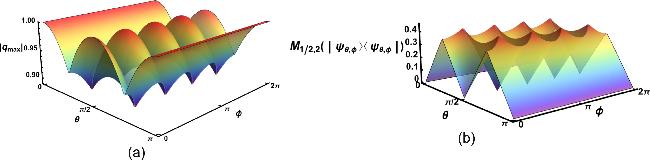
Figure 1. The surfaces of $| {q}_{{\rm{\max }}}| $ and ${M}_{1/2,2}\left(| {\psi }_{\theta ,\phi }\rangle \langle {\psi }_{\theta ,\phi }| \right)$ with the variation of θ ∈ [0, π] and φ ∈ [0, 2π), respectively.

Consider qutrit systems and note that

$\begin{eqnarray*}\begin{array}{rcl}{ \mathcal P }{{ \mathcal S }}_{3} & = & \left\{| 0\rangle ,| 1\rangle ,| 2\rangle \right\}\\ & & \cup \left\{\frac{| 0\rangle +{\omega }^{j}| 1\rangle +{\omega }^{k}| 2\rangle }{\sqrt{3}}:\omega ={\,\rm{e}\,}^{\frac{2\pi }{3}{\rm{i}}},j,k=0,1,2\right\}.\end{array}\end{eqnarray*}$

The qutrit T state is defined as $| T\rangle \,=\frac{1}{\sqrt{3}}\left({\,\rm{e}\,}^{\frac{2\pi }{9}{\rm{i}}}| 0\rangle +| 1\rangle +{\,\rm{e}\,}^{\frac{-2\pi }{9}{\rm{i}}}| 2\rangle \right).$ Then by direct calculations, we have

$\begin{eqnarray*}\begin{array}{rcl}| \langle m| T\rangle | & = & \frac{1}{\sqrt{3}},\\ | \langle {\psi }_{j,k}| T\rangle | & = & | {\,\rm{e}\,}^{\frac{2\pi }{9}{\rm{i}}}+{\,\rm{e}\,}^{-\frac{2\pi j}{3}{\rm{i}}}+{\,\rm{e}\,}^{\left(-\frac{2\pi }{9}-\frac{2\pi k}{3}\right){\rm{i}}}| ,\\ m,j,k & = & 0,1,2,\end{array}\end{eqnarray*}$
where $| {\psi }_{j,k}\rangle =\frac{| 0\rangle +{\omega }^{j}| 1\rangle +{\omega }^{k}| 2\rangle }{\sqrt{3}},j,k=0,1,2.$ Thus we obtain
$\begin{eqnarray*}\begin{array}{rcl}| {c}_{\max }| & = & {\rm{\max }}\left\{| \langle m| T\rangle | ,| \langle {\psi }_{j,k}| T\rangle | ,m,j,k=0,1,2\right\}\\ & = & | \langle {\psi }_{0,0}| T\rangle | =| \langle {\psi }_{0,2}| T\rangle | =| \langle {\psi }_{2,2}| T\rangle | \\ & = & \frac{1}{3}\left[1+{\rm{\cos }}\left(\frac{2\pi }{9}\right)\right].\end{array}\end{eqnarray*}$

By proposition 2, we have

$\begin{eqnarray}\begin{array}{rcl}{M}_{\alpha ,\beta }\left(| T\rangle \langle T| \right) & = & \frac{1}{(1-\alpha )\beta }\left\{\left[{\left(\frac{2}{3}+\frac{{\rm{\cos }}\left(\frac{2\pi }{9}\right)}{6}\right)}^{\alpha }\right.\right.\\ & & \left.{\left.+{\left(\frac{1}{3}-\frac{{\rm{\cos }}\left(\frac{2\pi }{9}\right)}{6}\right)}^{\alpha }\right]}^{\beta }-1\right\},\end{array}\end{eqnarray}$
and
$\begin{eqnarray}\begin{array}{rcl}{m}_{\alpha ,\beta }\left(| T\rangle \langle T| \right) & = & \frac{1}{(1-\alpha )\beta }\left\{1-\left[{\left(\frac{2}{3}+\frac{{\rm{\cos }}\left(\frac{2\pi }{9}\right)}{6}\right)}^{2-\alpha }\right.\right.\\ & & \left.{\left.+{\left(\frac{1}{3}-\frac{{\rm{\cos }}\left(\frac{2\pi }{9}\right)}{6}\right)}^{2-\alpha }\right]}^{\beta }\right\},\end{array}\end{eqnarray}$
for α ∈ (0, 1) ∪ (1, 2), β ∈ ( − , 0) ∪ (0, + ).

We depict ${M}_{\alpha ,\beta }\left(| T\rangle \langle T| \right)$ and ${m}_{\alpha ,\beta }\left(| T\rangle \langle T| \right)$ in equations (35) and (36) with α ∈ (0, 1) ∪ (1, 2) and β ∈ ( − 20, 0) ∪ (0, 20) in figure 2. It can be seen that ${M}_{\alpha ,\beta }\left(| T\rangle \langle T| \right)$ and ${m}_{\alpha ,\beta }\left(| T\rangle \langle T| \right)$ are highly symmetric in this parameter range.

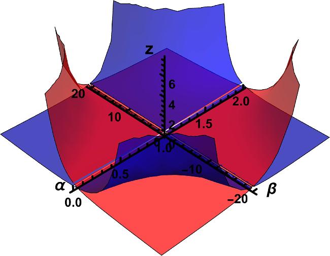
Figure 2. The red surface represents ${M}_{\alpha ,\beta }\left(| T\rangle \langle T| \right)$ and the blue surface represents ${m}_{\alpha ,\beta }\left(| T\rangle \langle T| \right)$ with α ∈ (0, 1) ∪ (1, 2) and β ∈ (−20, 0) ∪ (0, 20).

According to the proof of proposition
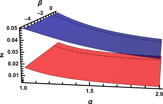
 5, we have

$\begin{eqnarray*}\begin{array}{r}\begin{array}{l}{M}_{\alpha ,\beta }({T}^{1/4}| {\psi }_{0}\rangle )-{M}_{\alpha ,\beta }(| {\psi }_{0}\rangle )\\ \quad =\frac{1}{(1-\alpha )\beta }\left\{{\left[{\cos }^{2\alpha }\left(\frac{3\pi }{64}\right)+{\sin }^{2\alpha }\left(\frac{3\pi }{64}\right)\right]}^{\beta }\right.\\ \qquad -\left.{\left[{\cos }^{2\alpha }\left(\frac{\pi }{32}\right)+{\sin }^{2\alpha }\left(\frac{\pi }{32}\right)\right]}^{\beta }\right\},\end{array}\end{array}\end{eqnarray*}$
and
$\begin{eqnarray*}\begin{array}{rcl}{{ \mathcal M }}_{\alpha ,\beta }({T}^{1/4}) & = & \frac{1}{(1-\alpha )\beta }\left\{\left[{\cos }^{2\alpha }\left(\frac{\pi }{64}\right)\right.\right.\\ & & \left.{\left.+{\sin }^{2\alpha }\left(\frac{\pi }{64}\right)\right]}^{\beta }-1\right\},\end{array}\end{eqnarray*}$
for α ∈ (1, 2) and β ∈ (−5, 0) ∪ (0, 1), where T is a qubit T-gate, and $| {\psi }_{0}\rangle =\frac{1}{\sqrt{2}}\left(| 0\rangle +{\,\rm{e}\,}^{\frac{\pi }{8}{\rm{i}}}| 1\rangle \right)$ in qubit systems.

We depict Mα,β(T1/4ψ0⟩) − Mα,β(∣ψ0⟩) and ${{ \mathcal M }}_{\alpha ,\beta }({T}^{1/4})$ with α ∈ (1, 2) and β ∈ (− 5, 0) ∪ (0, 1) in figure 3. It shows that Mα,β(T1/4ψ0⟩) − Mα,β(∣ψ0⟩) is always larger than ${{ \mathcal M }}_{\alpha ,\beta }({T}^{1/4})$ in this parameter range.

Figure 3. The blue surface represents Mα,β(T1/4ψ0⟩) − Mα,β(∣ψ0⟩) and the red surface represents ${{ \mathcal M }}_{\alpha ,\beta }({T}^{1/4})$ with α ∈ (1, 2) and β ∈ (−5, 0) ∪ (0, 1).

7. Summary

We have proposed two pure-state stabilizer monotones which can be calculated on low-dimensional systems for pure states. We have showed that the quantifier Mα,β(ρ) is bounded in qubit systems with α ∈ (0, 1) ∪ (1, + ) and β ∈ (−, 0) ∪ (0, + ), and the lower bound holds if and only if $\rho \in {{ \mathcal S }}_{d}$, while the upper bound holds if and only if ρ is a T-type state. We have also compared our magic quantifiers with other quantifiers, showing that Mα,β is controlled by some function of the robustness of magic R for pure states with α ∈ (0, 1) ∪ (1, + ), β ∈ (1, + ). As an application, we have proved that the initial nonstabilizerness in the input state can enhance the magic generating power in qubit systems when considering ${{ \mathcal M }}_{\alpha ,\beta }$ for α ∈ (1, 2), β ∈ (−, 0) ∪ (0, 1). Our results may shed some new light on the study of quantification of the magic at the level of quantum states, and may offer new perspective in the research of magic resource theory.

Author contributions

Linmao Wang wrote the main manuscript text and Zhaoqi Wu supervised and revised the manuscript. All authors reviewed the manuscript.

Competing interests

The authors declare no competing interests.

Appendix

Here we give the proof of propositions 15, theorems 15 and lemma 7.

A.1. Proof of proposition 1

Applying the spectral decomposition, we obtain
$\begin{eqnarray*}\begin{array}{r}\frac{| \psi \rangle \langle \psi | +| \phi \rangle \langle \phi | }{2}={\lambda }_{1}| {\xi }_{1}\rangle \langle {\xi }_{1}| +{\lambda }_{2}| {\xi }_{2}\rangle \langle {\xi }_{2}| ,\end{array}\end{eqnarray*}$
where
$\begin{eqnarray*}\begin{array}{rcl}{\lambda }_{1} & = & \frac{1+| \langle \psi | \phi \rangle | }{2},\,\,{\lambda }_{2}=\frac{1-| \langle \psi | \phi \rangle | }{2},\\ | {\xi }_{1}\rangle & = & \frac{| \psi \rangle +{\,\rm{e}\,}^{{\rm{i}}\theta }| \phi \rangle }{\sqrt{2(1+| s| )}},\,\,| {\xi }_{2}\rangle =\frac{| \psi \rangle -{\,\rm{e}\,}^{{\rm{i}}\theta }| \phi \rangle }{\sqrt{2(1-| s| )}},\\ s & = & \langle \phi | \psi \rangle ,\,\,s=| s| {\,\rm{e}\,}^{{\rm{i}}\theta },\theta \in {\mathbb{R}}.\end{array}\end{eqnarray*}$
Hence we have
$\begin{eqnarray}\begin{array}{l}{J}_{\alpha ,\beta }\left(| \psi \rangle \langle \psi | ,| \phi \rangle \langle \phi | \right)\\ ={S}_{\alpha ,\beta }\left(\frac{| \psi \rangle \langle \psi | +| \phi \rangle \langle \phi | }{2}\right)\\ -\frac{1}{2}{S}_{\alpha ,\beta }\left(| \psi \rangle \langle \psi | \right)\\ -\frac{1}{2}{S}_{\alpha ,\beta }\left(| \phi \rangle \langle \phi | \right)\\ ={S}_{\alpha ,\beta }\left(\frac{| \psi \rangle \langle \psi | +| \phi \rangle \langle \phi | }{2}\right)\\ ={H}_{\alpha ,\beta }\left\{\left(\frac{1+| \langle \psi | \phi \rangle | }{2},\frac{1-| \langle \psi | \phi \rangle | }{2}\right)\right\}\\ =\frac{1}{(1-\alpha )\beta }\left[{\left({\lambda }_{1}^{\alpha }+{\lambda }_{2}^{\alpha }\right)}^{\beta }-1\right],\end{array}\end{eqnarray}$
where
$\begin{eqnarray}{H}_{\alpha ,\beta }(\left\{{p}_{i}\right\})=\frac{1}{(1-\alpha )\beta }\left[{\left(\displaystyle \sum _{j}^{}{p}_{i}^{\alpha }\right)}^{\beta }-1\right]\end{eqnarray}$
is the unified (αβ)-entropy [52].
Noting that
$\begin{eqnarray*}\begin{array}{r}| \langle \psi | {\xi }_{i}\rangle {| }^{2}=| \langle \phi | {\xi }_{i}\rangle {| }^{2}={\lambda }_{i},i=1,2,\end{array}\end{eqnarray*}$
we have
$\begin{eqnarray}\begin{array}{l}{D}_{\alpha ,\beta }\left(| \psi \rangle \langle \psi | \parallel \frac{| \psi \rangle \langle \psi | +| \phi \rangle \langle \phi | }{2}\right)\\ =\frac{1}{(1-\alpha )\beta }\left\{1-{\left[{\rm{Tr}}\left((| \psi \rangle \langle \psi | {)}^{\alpha }{\left(\frac{| \psi \rangle \langle \psi | +| \phi \rangle \langle \phi | }{2}\right)}^{1-\alpha }\right)\right]}^{\beta }\right\}\\ =\frac{1}{(1-\alpha )\beta }\left[1-{\left({\lambda }_{1}^{1-\alpha }| \langle \psi | {\xi }_{1}\rangle {| }^{2}+{\lambda }_{2}^{1-\alpha }| \langle \psi | {\xi }_{2}\rangle {| }^{2}\right)}^{\beta }\right]\\ =\frac{1}{(1-\alpha )\beta }\left[1-{\left({\lambda }_{1}^{2-\alpha }+{\lambda }_{2}^{2-\alpha }\right)}^{\beta }\right],\end{array}\end{eqnarray}$
and
$\begin{eqnarray}\begin{array}{l}{D}_{\alpha ,\beta }\left(| \phi \rangle \langle \phi | \parallel \frac{| \psi \rangle \langle \psi | +| \phi \rangle \langle \phi | }{2}\right)\\ =\frac{1}{(1-\alpha )\beta }\left\{1-{\left[{\rm{Tr}}\left((| \phi \rangle \langle \phi | {)}^{\alpha }{\left(\frac{| \psi \rangle \langle \psi | +| \phi \rangle \langle \phi | }{2}\right)}^{1-\alpha }\right)\right]}^{\beta }\right\}\\ =\frac{1}{(1-\alpha )\beta }\left[1-{\left({\lambda }_{1}^{1-\alpha }| \langle \phi | {\xi }_{1}\rangle {| }^{2}+{\lambda }_{2}^{1-\alpha }| \langle \phi | {\xi }_{2}\rangle {| }^{2}\right)}^{\beta }\right]\\ =\frac{1}{(1-\alpha )\beta }\left[1-{\left({\lambda }_{1}^{2-\alpha }+{\lambda }_{2}^{2-\alpha }\right)}^{\beta }\right].\end{array}\end{eqnarray}$
Combining equations (A3) and (A4), we obtain
$\begin{eqnarray}{J}_{\alpha ,\beta }^{{\prime} }\left(| \psi \rangle \langle \psi | ,| \phi \rangle \langle \phi | \right)=\frac{1}{(1-\alpha )\beta }\left[1-{\left({\lambda }_{1}^{2-\alpha }+{\lambda }_{2}^{2-\alpha }\right)}^{\beta }\right],\end{eqnarray}$
and thus we get
$\begin{eqnarray*}\begin{array}{r}{J}_{\alpha ,\beta }\left(| \psi \rangle \langle \psi | ,| \phi \rangle \langle \phi | \right)={J}_{2-\alpha ,\beta }^{{\prime} }\left(| \psi \rangle \langle \psi | ,| \phi \rangle \langle \phi | \right),\end{array}\end{eqnarray*}$
for all α ∈ (0, 1) ∪ (1, 2) and β ∈ ( − , 0) ∪ (0, + ) by comparing equations (A1) and (A5). Thus we complete the proof. □

A.2. Proof of theorem 1

(i)–(iii) can be directly proved by applying lemma 1, and (iv) is obvious from the definition of Jα,β(ρσ), so we only prove item (v).
For α ∈ (1, + ), β ∈ [1, + ), we have
$\begin{eqnarray*}\begin{array}{r}\begin{array}{l}| {J}_{\alpha ,\beta }({\rho }_{1},\sigma )-{J}_{\alpha ,\beta }({\rho }_{2},\sigma )| \\ =\left|{S}_{\alpha ,\beta }\left(\frac{{\rho }_{1}+\sigma }{2}\right)-{S}_{\alpha ,\beta }\left(\frac{{\rho }_{2}+\sigma }{2}\right)\right.\\ \left.+\frac{1}{2}{S}_{\alpha ,\beta }({\rho }_{2})-\frac{1}{2}{S}_{\alpha ,\beta }({\rho }_{1})\right|\\ \leqslant \left|{S}_{\alpha ,\beta }\left(\frac{{\rho }_{1}+\sigma }{2}\right)-{S}_{\alpha ,\beta }\left(\frac{{\rho }_{2}+\sigma }{2}\right)\right|\\ +\frac{1}{2}\left|{S}_{\alpha ,\beta }({\rho }_{2})-{S}_{\alpha ,\beta }({\rho }_{1})\right|\\ \leqslant \frac{\alpha }{\alpha -1}{\parallel \frac{{\rho }_{1}-{\rho }_{2}}{2}\parallel }_{1}+\frac{\alpha }{2(\alpha -1)}{\parallel {\rho }_{2}-{\rho }_{1}\parallel }_{1}\\ =\frac{\alpha }{\alpha -1}{\parallel {\rho }_{1}-{\rho }_{2}\parallel }_{1},\end{array}\end{array}\end{eqnarray*}$
where the first equality follows from equation (1), the second inequality comes from lemma 1 (iv), and the second equality follows from the linearity of the trace distance.
In a similar manner, we can prove that $| {J}_{\alpha ,\beta }(\rho ,{\sigma }_{1})\,-{J}_{\alpha ,\beta }(\rho ,{\sigma }_{2})| \leqslant \frac{\alpha }{\alpha -1}\parallel {\sigma }_{1}-{\sigma }_{2}{\parallel }_{1}$ for α ∈ (1, + ), β ∈ [1, + ). □

A.3. Proof of theorem 2

We can prove (iii)–(v) by lemma 2 (iii)–(v) respectively and (vi) can be obtained by definition, so we only prove (i) and (ii).
For item (i), by lemma 2 (i), we have ${J}_{\alpha ,\beta }^{{\prime} }(\rho ,\sigma )\geqslant 0$ for α ∈ (0, 1) ∪ (1, + ), β ∈ ( − , 0) ∪ (0, + ) and the inequality saturates if and only if
$\begin{eqnarray*}\begin{array}{r}{D}_{\alpha ,\beta }\left(\rho \parallel \frac{\rho +\sigma }{2}\right)=0={D}_{\alpha ,\beta }\left(\sigma \parallel \frac{\rho +\sigma }{2}\right),\end{array}\end{eqnarray*}$
which is equivalent to ρ = σ.
For item (ii), we have
$\begin{eqnarray*}\begin{array}{l}{J}_{\alpha ,\beta }^{{\prime} }(\rho \displaystyle \otimes \tau ,\sigma \displaystyle \otimes \tau )\\ =\frac{1}{2}\left[{D}_{\alpha ,\beta }\left(\rho \displaystyle \otimes \tau \parallel \frac{\rho +\sigma }{2}\displaystyle \otimes \tau \right)\right.\\ +\left.{D}_{\alpha ,\beta }\left(\sigma \displaystyle \otimes \tau \parallel \frac{\rho +\sigma }{2}\displaystyle \otimes \tau \right)\right]\\ =\frac{1}{2}\left[{D}_{\alpha ,\beta }\left(\rho \parallel \frac{\rho +\sigma }{2}\right)+(\alpha -1)\beta \right.\\ \left.{D}_{\alpha ,\beta }\,\left(\rho \parallel \frac{\rho +\sigma }{2}\right){D}_{\alpha ,\beta }\left(\tau \parallel \tau \right)\right]\\ +\frac{1}{2}\left[{D}_{\alpha ,\beta }\left(\sigma \parallel \frac{\rho +\sigma }{2}\right)\right.\\ +\left.(\alpha -1)\beta {D}_{\alpha ,\beta }\left(\sigma \parallel \frac{\rho +\sigma }{2}\right){D}_{\alpha ,\beta }\left(\,{,}(,\tau \parallel \tau \right)\Space{0ex}{3.25ex}{0ex}\right]\\ =\frac{1}{2}\left[{D}_{\alpha ,\beta }\left(\rho \parallel \frac{\rho +\sigma }{2}\right)+{D}_{\alpha ,\beta }\left(\sigma \parallel \frac{\rho +\sigma }{2}\right)\right]\\ ={J}_{\alpha ,\beta }^{{\prime} }(\rho ,\sigma ),\end{array}\end{eqnarray*}$
with α ∈ (0, 1) ∪ (1, + ), β ∈ ( − , 0) ∪ (0, + ), where the first and last equality comes from equation (2), the second equality follows from lemma 2 (ii), and the third holds due to Dα,β(ττ) = 0. □

A.4. Proof of theorem 3

We only prove item (iv) and (vi), the other properties can be easily derived by imitating the proof of proposition 1 in [40].
For item (iv), suppose that α ∈ (1, 2), β ∈ ( − , 1]. Then we have
$\begin{eqnarray*}\begin{array}{r}\begin{array}{l}{M}_{\alpha ,\beta }\left({ \mathcal E }\left(| \psi \rangle \langle \psi | \right)\right)\\ =\mathop{\min }\limits_{| \phi \rangle \in { \mathcal P }{{ \mathcal S }}_{d}}{J}_{\alpha ,\beta }\left({ \mathcal E }\left(| \psi \rangle \langle \psi | \right),| \phi \rangle \langle \phi | \right)\\ \leqslant \mathop{\min }\limits_{| \phi \rangle \in { \mathcal P }{{ \mathcal S }}_{d}}{J}_{\alpha ,\beta }\left({ \mathcal E }\left(| \psi \rangle \langle \psi | \right),{ \mathcal E }(| \phi \rangle \langle \phi | )\right)\\ \leqslant \mathop{\min }\limits_{| \phi \rangle \in { \mathcal P }{{ \mathcal S }}_{d}}{J}_{\alpha ,\beta }\left(| \psi \rangle \langle \psi | ,| \phi \rangle \langle \phi | \right)\\ ={M}_{\alpha ,\beta }\left(| \psi \rangle \langle \psi | \right),\end{array}\end{array}\end{eqnarray*}$
where the first equality holds by using equation (5) and the fact that any stabilizer operation ${ \mathcal E }$ maps pure states to pure states, the first inequality is true since stabilizer operation preserves stabilizer states and the second inequality follows from remark 2.
For item (vi), suppose that α ∈ (1, + ), β ∈ [1, + ). Then we have
$\begin{eqnarray*}\begin{array}{r}\begin{array}{l}{M}_{\alpha ,\beta }(| {\psi }_{1}\rangle \langle {\psi }_{1}| )-{M}_{\alpha ,\beta }(| {\psi }_{2}\rangle \langle {\psi }_{2}| )\\ =\mathop{\min }\limits_{| \phi \rangle \in { \mathcal P }{{ \mathcal S }}_{d}}{J}_{\alpha ,\beta }\left(| {\psi }_{1}\rangle \langle {\psi }_{1}| ,| \phi \rangle \langle \phi | \right)\\ -{J}_{\alpha ,\beta }\left(| {\psi }_{2}\rangle \langle {\psi }_{2}| ,| {\phi }_{2}\rangle \langle {\phi }_{2}| \right)\\ \leqslant {J}_{\alpha ,\beta }\left(| {\psi }_{1}\rangle \langle {\psi }_{1}| ,| {\phi }_{2}\rangle \langle {\phi }_{2}| \right)\\ -{J}_{\alpha ,\beta }\left(| {\psi }_{2}\rangle \langle {\psi }_{2}| ,| {\phi }_{2}\rangle \langle {\phi }_{2}| \right)\\ \leqslant | {J}_{\alpha ,\beta }\left(| {\psi }_{1}\rangle \langle {\psi }_{1}| ,| {\phi }_{2}\rangle \langle {\phi }_{2}| \right)\\ -{J}_{\alpha ,\beta }\left(| {\psi }_{2}\rangle \langle {\psi }_{2}| ,| {\phi }_{2}\rangle \langle {\phi }_{2}| \right)| \\ \leqslant \frac{\alpha }{\alpha -1}\parallel | {\psi }_{1}\rangle \langle {\psi }_{1}| -| {\psi }_{2}\rangle \langle {\psi }_{2}| {\parallel }_{1},\end{array}\end{array}\end{eqnarray*}$
where the first equality holds because we assume that ∣φ2⟩ reaches the minimum in the definition of Mα,β(∣ψ2⟩⟨ψ2∣), the last inequality comes from theorem 1 (v). Similarly, we can obtain that Mα,β(∣ψ2⟩⟨ψ2∣) − Mα,β(∣ψ1⟩⟨ψ1∣)≤ $\frac{\alpha }{\alpha -1}\parallel | {\psi }_{1}\rangle \langle $ψ1∣ − ∣ψ2⟩⟨ψ2∣∥1, and thus we have
$\begin{eqnarray*}\begin{array}{r}\begin{array}{l}| {M}_{\alpha ,\beta }(| {\psi }_{1}\rangle \langle {\psi }_{1}| )-{M}_{\alpha ,\beta }(| {\psi }_{2}\rangle \langle {\psi }_{2}| )| \\ \quad \leqslant \frac{\alpha }{\alpha -1}\parallel | {\psi }_{1}\rangle \langle {\psi }_{1}| -| {\psi }_{2}\rangle \langle {\psi }_{2}| {\parallel }_{1},\end{array}\end{array}\end{eqnarray*}$
which completes the proof. □

A.5. Proof of proposition 2

For α ∈ (0, 1), β ∈ ( − , 0) ∪ (0, + ), we have
$\begin{eqnarray*}\begin{array}{r}\begin{array}{l}{M}_{\alpha ,\beta }\left(| \psi \rangle \langle \psi | \right)\\ =\mathop{\min }\limits_{| \phi \rangle \in { \mathcal P }{{ \mathcal S }}_{d}}\left\{\frac{1}{(1-\alpha )\beta }\left[\left({\left(\frac{1+| \langle \phi | \psi \rangle | }{2}\right)}^{\alpha }\right.\right.\right.\\ \left.\left.{\left.+{\left(\frac{1-| \langle \phi | \psi \rangle | }{2}\right)}^{\alpha }\right)}^{\beta }-1\right]\right\}\\ =\frac{1}{(1-\alpha )\beta }\left\{\left[\mathop{\min }\limits_{| \phi \rangle \in { \mathcal P }{{ \mathcal S }}_{d}}\left({\left(\frac{1+| \langle \phi | \psi \rangle | }{2}\right)}^{\alpha }\right.\right.\right.\\ \left.{\left.\left.+{\left(\frac{1-| \langle \phi | \psi \rangle | }{2}\right)}^{\alpha }\right)\right]}^{\beta }-1\right\}\\ =\frac{1}{(1-\alpha )\beta }\left\{{\left[{\left(\frac{1+| {c}_{\psi }| }{2}\right)}^{\alpha }+{\left(\frac{1-| {c}_{\psi }| }{2}\right)}^{\alpha }\right]}^{\beta }-1\right\},\end{array}\end{array}\end{eqnarray*}$
the first equality follows from the definition of ${M}_{\alpha ,\beta }\left(| \psi \rangle \langle \psi | \right)$, the second equality comes from lemma 3(i) and the third follows from lemma 4.
For α ∈ (1, + ), β ∈ ( − , 0) ∪ (0, + ), we only need to replace min with max in the second equality to obtain the same conclusion. Thus we complete the proof. □

A.6. Proof of proposition 3

We only consider the case in which α ∈ (1, + ), while the proof is similar when α ∈ (0, 1). Denote
$\begin{eqnarray*}\begin{array}{r}h(\lambda ,\alpha ,\beta )=\frac{1}{(1-\alpha )\beta }\left\{{\left[{\lambda }^{\alpha }+{\left(1-\lambda \right)}^{\alpha }\right]}^{\beta }-1\right\}.\end{array}\end{eqnarray*}$
For α ∈ (1, + ), by applying lemma 6, we have
$\begin{eqnarray*}\begin{array}{r}\left[{(2\lambda -1)}^{2}+h(\lambda ,\alpha ,\beta )\right]\leqslant \mathop{\mathrm{lim}}\limits_{\beta \to {1}^{+}}\left[{(2\lambda -1)}^{2}+h(\lambda ,\alpha ,\beta )\right].\end{array}\end{eqnarray*}$
Then by lemma 5 and proposition 3 in [40], we obtain
$\begin{eqnarray*}\begin{array}{r}\begin{array}{l}\mathop{\mathrm{lim}}\limits_{\beta \to {1}^{+}}\left[{(2\lambda -1)}^{2}+h(\lambda ,\alpha ,\beta )\right]\\ \leqslant \mathop{\mathrm{lim}}\limits_{\alpha \to {1}^{+}}\mathop{\mathrm{lim}}\limits_{\beta \to {1}^{+}}\left[{(2\lambda -1)}^{2}+h(\lambda ,\alpha ,\beta )\right]\leqslant {t}_{0},\end{array}\end{array}\end{eqnarray*}$
which yields
$\begin{eqnarray*}\begin{array}{r}\left[{(2\lambda -1)}^{2}+h(\lambda ,\alpha ,\beta )\right]\leqslant {t}_{0}.\end{array}\end{eqnarray*}$
From the definition of ${M}_{\alpha ,\beta }\left(| \psi \rangle \langle \psi | \right)$ and $F\left(| \psi \rangle \langle \psi | \right)$, we obtain
$\begin{eqnarray*}\begin{array}{r}{M}_{\alpha ,\beta }\left(| \psi \rangle \langle \psi | \right)+F\left(| \psi \rangle \langle \psi | \right)\leqslant {t}_{0},\end{array}\end{eqnarray*}$
thus
$\begin{eqnarray*}\begin{array}{r}\begin{array}{l}{M}_{\alpha ,\beta }\left(| \psi \rangle \langle \psi | \right)+\frac{1}{1+R\left(| \psi \rangle \langle \psi | \right)}\\ \quad \leqslant {M}_{\alpha ,\beta }\left(| \psi \rangle \langle \psi | \right)+F\left(| \psi \rangle \langle \psi | \right)\leqslant {t}_{0},\end{array}\end{array}\end{eqnarray*}$
which completes the proof. □

A.7. Proof of theorem 5

Items (i) and (ii) are obvious from the definition, so we only prove item (iii).
For α ∈ (1, 2), β ∈ ( − , 0) ∪ (0, 1], we have
$\begin{eqnarray*}\begin{array}{r}\begin{array}{l}{{ \mathcal M }}_{\alpha ,\beta }({U}_{1}\displaystyle \otimes {U}_{2})\\ =\mathop{\max }\limits_{\rho \in {{ \mathcal S }}_{{d}^{2}}}{M}_{\alpha ,\beta }\left[({U}_{1}\displaystyle \otimes {U}_{2})\rho ({U}_{1}^{\dagger }\displaystyle \otimes {U}_{2}^{\dagger })\right]\\ \geqslant \mathop{\max }\limits_{{\rho }_{1},{\rho }_{2}\in {{ \mathcal S }}_{d}}{M}_{\alpha ,\beta }\left[({U}_{1}\displaystyle \otimes {U}_{2})\left({\rho }_{1}\displaystyle \otimes {\rho }_{2}\right)({U}_{1}^{\dagger }\displaystyle \otimes {U}_{2}^{\dagger })\right]\\ =\mathop{\max }\limits_{{\rho }_{1},{\rho }_{2}\in {{ \mathcal S }}_{d}}{M}_{\alpha ,\beta }\left[\left({U}_{1}{\rho }_{1}{U}_{1}^{\dagger }\right)\displaystyle \otimes \left({U}_{2}{\rho }_{2}{U}_{2}^{\dagger }\right)\right]\\ \geqslant \mathop{\max }\limits_{{\rho }_{1}\in {{ \mathcal S }}_{d}}{M}_{\alpha ,\beta }\left({U}_{1}{\rho }_{1}{U}_{1}^{\dagger }\right)\\ ={{ \mathcal M }}_{\alpha ,\beta }\left({U}_{1}\right),\end{array}\end{array}\end{eqnarray*}$
where the first equality holds due to equation (23), the first inequality is true since ${{ \mathcal S }}_{d}\otimes {{ \mathcal S }}_{d}\subseteq {{ \mathcal S }}_{{d}^{2}}$, and the second inequality follows from theorem 3 (v).

A.8. Proof of proposition 4

For α ∈ (0, 1), β ∈ ( − , 0) ∪ (0, + ), we have
$\begin{eqnarray*}\begin{array}{r}\begin{array}{l}{{ \mathcal M }}_{\alpha ,\beta }(U)\\ =\mathop{\max }\limits_{| \phi \rangle \in { \mathcal P }{{ \mathcal S }}_{d}}{M}_{\alpha ,\beta }(U| \phi \rangle \langle \phi | {U}^{\dagger })\\ =\mathop{\max }\limits_{| \phi \rangle \in { \mathcal P }{{ \mathcal S }}_{d}}\mathop{\min }\limits_{| \psi \rangle \in { \mathcal P }{{ \mathcal S }}_{d}}\left\{\frac{1}{(1-\alpha )\beta }\left[\left({\left(\frac{1+| \langle \psi | U| \phi \rangle | }{2}\right)}^{\alpha }\right.\right.\right.\\ \left.\left.{\left.+{\left(\frac{1-| \langle \psi | U| \phi \rangle | }{2}\right)}^{\alpha }\right)}^{\beta }-1\right]\right\}\\ =\frac{1}{(1-\alpha )\beta }\left\{{\left[{\left(\frac{1+| {C}_{U}| }{2}\right)}^{\alpha }+{\left(\frac{1-| {C}_{U}| }{2}\right)}^{\alpha }\right]}^{\beta }-1\right\},\end{array}\end{array}\end{eqnarray*}$
where the first equality follows from the fact that ${{ \mathcal S }}_{d}$ is a convex set, the second equation comes from the definition, and the last follows from lemma 3(i) and lemma 4.
It can be easily verified that the conclusion also holds for α ∈ (1, + ), β ∈ ( − , 0) ∪ (0, + ). Hence we complete the proof. □

A.9. Proof of lemma 7

(i) For $\alpha \in (1,2),x\in (0,\frac{\pi }{4})$, it follows that
$\begin{eqnarray*}\begin{array}{rcl}\frac{\partial w(x,\alpha )}{\partial x} & = & 2\alpha \cdot {\rm{\sin }}x\cdot {\rm{\cos }}x\\ & & \times \left({{\rm{\sin }}}^{2\alpha -2}x-{{\rm{\cos }}}^{2\alpha -2}x\right)\lt 0.\end{array}\end{eqnarray*}$
(ii) For $\alpha \in (1,2),x\in (0,\frac{\pi }{16}]$, we obtain
$\begin{eqnarray*}\begin{array}{rcl}\frac{{\partial }^{2}w(x,\alpha )}{\partial {x}^{2}} & = & 2\alpha \left\{(2\alpha -1)[{\sin }^{2\alpha -2}x{\cos }^{2}x\right.\\ & & \left.+{\cos }^{2\alpha -2}x{\sin }^{2}x]-({\sin }^{2\alpha }x+{\cos }^{2\alpha }x)\right\}.\end{array}\end{eqnarray*}$
Let $t={\tan }^{2}x\in \left(0,{t}_{\max }\right]$, where ${t}_{\max }={\tan }^{2}\frac{\pi }{16}$. Then we have
$\begin{eqnarray*}\begin{array}{r}\frac{{\partial }^{2}w(x,\alpha )}{\partial {x}^{2}}=G(t,\alpha )=(2\alpha -1)\left({t}^{\alpha -1}+t\right)-\left({t}^{\alpha }+1\right).\end{array}\end{eqnarray*}$
We next show that G(tα) < 0 for all $t\in (0,{t}_{\max }]$ and α ∈ (1, 2).
By taking the partial derivative of G(tα) with respect to t, we obtain
$\begin{eqnarray*}\begin{array}{rcl}\frac{\partial G(t,\alpha )}{\partial t} & = & (2\alpha -1)(\alpha -1){t}^{\alpha -2}+2\alpha -1-\alpha {t}^{\alpha -1}\\ & \geqslant & (2\alpha -1)(\alpha -1)+2\alpha -1-\alpha {t}^{\alpha -1}\\ & = & (2\alpha -1)(\alpha -1)+\left[\alpha (2-{t}^{\alpha -1})-1\right]\gt 0.\end{array}\end{eqnarray*}$
Then for all α ∈ (1, 2), $G{(t,\alpha )}_{\max }\,=$ $G({t}_{\max },\alpha )\,=$ $(2\alpha -1)\left({t}_{\max }^{\alpha -1}+{t}_{\max }\right)-$ $\left({t}_{\max }^{\alpha }+1\right).$ So we only need to prove $G({t}_{\max },\alpha )\lt 0$ for all α ∈ (1, 2).
In fact, by taking the first and second derivative of $G({t}_{\max },\alpha )$, we have
$\begin{eqnarray*}\begin{array}{rcl}G^{\prime} ({t}_{\max },\alpha ) & = & 2\left({t}_{\max }^{\alpha -1}+{t}_{\max }\right)\\ & & +{\mathrm{ln}}{t}_{\max }\left[(2\alpha -1){t}_{\max }^{\alpha -1}-{t}_{\max }^{\alpha }\right],\end{array}\end{eqnarray*}$
$\begin{eqnarray*}\begin{array}{r}{G}^{{\prime\prime} }({t}_{\max },\alpha )={t}_{\max }^{\alpha -1}{\mathrm{ln}}{t}_{\max }\left[(2\alpha -1-{t}_{\max }){\mathrm{ln}}{t}_{\max }+4\right].\end{array}\end{eqnarray*}$
Noting that
$\begin{eqnarray*}\begin{array}{r}{G}^{{\prime\prime} }({t}_{\max },\alpha )\gt 0\,\,{\rm{for}}\,\,\alpha \in \left(\frac{1+{t}_{\max }}{2}-\frac{2}{{\mathrm{ln}}{t}_{\max }},2\right),\end{array}\end{eqnarray*}$
and
$\begin{eqnarray*}\begin{array}{r}{G}^{{\prime\prime} }({t}_{\max },\alpha )\lt 0\,\,{\rm{for}}\,\,\alpha \in \left(1,\frac{1+{t}_{\max }}{2}-\frac{2}{{\mathrm{ln}}{t}_{\max }}\right),\end{array}\end{eqnarray*}$
we have
$\begin{eqnarray*}\begin{array}{rcl}G^{\prime} {({t}_{\max },\alpha )}_{\max } & = & \max \left\{G^{\prime} ({t}_{\max },1),G^{\prime} ({t}_{\max },2)\right\}\\ & = & G^{\prime} ({t}_{\max },2)\approx -0.2205\lt 0,\end{array}\end{eqnarray*}$
and so
$\begin{eqnarray*}\begin{array}{r}G({t}_{\max },\alpha )\lt \mathop{\mathrm{lim}}\limits_{\alpha \to {0}^{+}}G({t}_{\max },\alpha )=0\end{array},\end{eqnarray*}$
for all α ∈ (1, 2). Thus we complete the proof. □

A.10. Proof of proposition 5

Consider the unitary gate
$\begin{eqnarray*}\begin{array}{r}{U}_{0}={T}^{1/4}=\left[\begin{array}{cc}1 & 0\\ 0 & {\,\rm{e}\,}^{\frac{\pi }{16}{\rm{i}}}\end{array}\right],\end{array}\end{eqnarray*}$
and the input state $| {\psi }_{0}\rangle =\frac{1}{\sqrt{2}}\left(| 0\rangle +{\,\rm{e}\,}^{\frac{\pi }{8}{\rm{i}}}| 1\rangle \right).$
By proposition 1 and proposition 4, we obtain
$\begin{eqnarray*}\begin{array}{rcl}{{ \mathcal M }}_{\alpha ,\beta }({T}^{1/4}) & = & \frac{1}{(1-\alpha )\beta }\\ & & \times \left\{{\left[{\cos }^{2\alpha }\left(\frac{\pi }{64}\right)+{\sin }^{2\alpha }\left(\frac{\pi }{64}\right)\right]}^{\beta }-1\right\},\end{array}\end{eqnarray*}$
$\begin{eqnarray*}\begin{array}{l}{M}_{\alpha ,\beta }({T}^{1/4}| {\psi }_{0}\rangle )=\frac{1}{(1-\alpha )\beta }\\ \,\times \,\left\{{\left[{\cos }^{2\alpha }\left(\frac{3\pi }{64}\right)+{\sin }^{2\alpha }\left(\frac{3\pi }{64}\right)\right]}^{\beta }-1\right\},\end{array}\end{eqnarray*}$
and
$\begin{eqnarray*}\begin{array}{rcl}{M}_{\alpha ,\beta }(| {\psi }_{0}\rangle ) & = & \frac{1}{(1-\alpha )\beta }\\ & & \times \left\{{\left[{\cos }^{2\alpha }\left(\frac{\pi }{32}\right)+{\sin }^{2\alpha }\left(\frac{\pi }{32}\right)\right]}^{\beta }-1\right\}.\end{array}\end{eqnarray*}$
Denote
$\begin{eqnarray*}\begin{array}{rcl}N(x,\alpha ,\beta ) & = & \frac{1}{(1-\alpha )\beta }\left[{\left({{\rm{\cos }}}^{2\alpha }x+{{\rm{\sin }}}^{2\alpha }x\right)}^{\beta }-1\right]\\ & = & g\left[w(x,\alpha ),\alpha ,\beta \right],\end{array}\end{eqnarray*}$
and
$\begin{eqnarray*}\begin{array}{rcl}K(x,\alpha ,\beta ) & = & N\left(x+\frac{\pi }{32},\alpha ,\beta \right)-N(x,\alpha ,\beta )\\ & & -N\left(\frac{\pi }{32},\alpha ,\beta \right),\end{array}\end{eqnarray*}$
where g(xαβ) and w(xα) are defined in lemma 3 and lemma 7, respectively.
Thus we have
$\begin{eqnarray*}\begin{array}{r}\begin{array}{l}{M}_{\alpha ,\beta }({T}^{1/4}| {\psi }_{0}\rangle )-{M}_{\alpha ,\beta }(| {\psi }_{0}\rangle )-{{ \mathcal M }}_{\alpha ,\beta }({T}^{1/4})\\ \quad =K\left(\frac{\pi }{64},\alpha ,\beta \right).\end{array}\end{array}\end{eqnarray*}$
Now we prove that $K(\frac{\pi }{64},\alpha ,\beta )\gt 0$ for all α ∈ (1, 2) and β ∈ ( − , 0) ∪ (0, 1). 
Taking the second-order partial derivative of N(xαβ) with respect to x, we obtain
$\begin{eqnarray*}\begin{array}{rcl}\frac{{\partial }^{2}N(x,\alpha ,\beta )}{\partial {x}^{2}} & = & \frac{{\partial }^{2}g[w(x,\alpha ),\alpha ,\beta ]}{\partial {[w(x,\alpha )]}^{2}}{\left[\frac{\partial w(x,\alpha )}{\partial x}\right]}^{2}\\ & & +\frac{{\partial }^{2}w(x,\alpha )}{\partial {x}^{2}}\frac{\partial g[w(x,\alpha ),\alpha ,\beta ]}{\partial w(x,\alpha )}.\end{array}\end{eqnarray*}$
For α ∈ (1, 2), β ∈ ( − , 0) ∪ (0, 1) and $x\in (0,\frac{\pi }{16})$, it follows from lemma 3 and lemma 7 that
$\begin{eqnarray*}\begin{array}{r}\begin{array}{l}\frac{{\partial }^{2}g[w(x,\alpha ),\alpha ,\beta ]}{\partial {[w(x,\alpha )]}^{2}}\gt 0,{\left[\frac{\partial w(x,\alpha )}{\partial x}\right]}^{2}\gt 0,\\ \frac{{\partial }^{2}w(x,\alpha )}{\partial {x}^{2}}\lt 0,\frac{\partial g[w(x,\alpha ),\alpha ,\beta ]}{\partial w(x,\alpha )}\lt 0.\end{array}\end{array}\end{eqnarray*}$
Then we have
$\begin{eqnarray*}\begin{array}{r}\frac{{\partial }^{2}N(x,\alpha ,\beta )}{\partial {x}^{2}}\gt 0,\end{array}\end{eqnarray*}$
and therefore
$\begin{eqnarray*}\begin{array}{r}\frac{\partial K(x,\alpha ,\beta )}{\partial x}=\frac{\partial N(x+\frac{\pi }{32},\alpha ,\beta )}{\partial x}-\frac{\partial N(x,\alpha ,\beta )}{\partial x}\gt 0,\end{array}\end{eqnarray*}$
which implies that K(xαβ) is strictly monotonically increasing with respect to $x\in (0,\frac{\pi }{16}]$. Hence we have
$\begin{eqnarray*}\begin{array}{r}K\left(\frac{\pi }{64},\alpha ,\beta \right)\gt K(0,\alpha ,\beta )=0,\end{array}\end{eqnarray*}$
which completes the proof. □

This work was supported by National Natural Science Foundation of China (Grant Nos. 12561084, 12161056) and Natural Science Foundation of Jiangxi Province of China (Grant No. 20232ACB211003).

1
Gottesman D 1997 Stabilizer codes and quantum error correction PhD Thesis California Institute of Technology

2
Gottesman D 1999 The Heisenberg representation of quantum computers Proceedings of the XXII International Colloquium on Group Theoretical Methods in Physics, 32-43

3
Gottesman D, Chuang I L 1999 Demonstrating the viability of universal quantum computation using teleportation and single-qubit operations Nature 402 390

DOI

4
Aaronson S, Gottesman D 2004 Improved simulation of stabilizer circuits Phys. Rev. A 70 052328

DOI

5
Veitch V, Mousavian S H, Gottesman D, Emerson J 2014 The resource theory of stabilizer quantum computation New J. Phys. 16 013009

DOI

6
Veitch V, Ferrie C, Gross D, Emerson J 2012 Negative quasi-probability as a resource for quantum computation New J. Phys. 14 113011

DOI

7
Bravyi S, Haah J 2012 Magic-state distillation with low overhead Phys. Rev. A 86 052329

DOI

8
Anwar H, Campbell E T, Browne D E 2012 Qutrit magic state distillation New J. Phys. 14 063006

DOI

9
Campbell E T, Anwar H, Browne D E 2012 Magic-state distillation in all prime dimensions using quantum Reed–Muller codes Phys. Rev. X 2 041021

DOI

10
Campbell E T, Howard M 2017 Unifying gate synthesis and magic state distillation Phys. Rev. Lett. 118 060501

DOI

11
Dawkins H, Howard M 2015 Qutrit magic state distillation tight in some directions Phys. Rev. Lett. 115 030501

DOI

12
Meier A M, Eastin B, Knill E 2012 Magic state distillation with the four-qubit code Quantum Inf. Comput. 13 195

DOI

13
Wang X, Wilde M M, Su Y 2020 Efficiently computable bounds for magic state distillation Phys. Rev. Lett. 124 090505

DOI

14
Peres A 1996 Separability criterion for density matrices Phys. Rev. Lett. 77 1413

DOI

15
Horodecki M, Horodecki P, Horodecki 1998 Mixed-state entanglement and distillation: is there a ‘bound' entanglement in nature? Phys. Rev. Lett. 80 5239

DOI

16
Rains E M 2002 A semidefinite program for distillable entanglement IEEE Trans. Inf. Theory 47 2921

DOI

17
Wang X, Duan R 2016 Improved semidefinite programming upper bound on distillable entanglement Phys. Rev. A 94 050301

DOI

18
Wang X, Duan R 2017 Nonadditivity of Rains' bound for distillable entanglement Phys. Rev. A 95 062322

DOI

19
Fang K, Wang X, Tomamichel M, Duan R 2019 Non-asymptotic entanglement distillation IEEE Trans. Inf. Theory 65 6454

DOI

20
Howard M, Campbell E 2017 Application of a resource theory for magic states to fault-tolerant quantum computing Phys. Rev. Lett. 118 090501

DOI

21
Heinrich M, Gross D 2019 Robustness of magic and symmetries of the stabiliser polytope Quantum 3 132

DOI

22
Liu Z, Winter A 2022 Many-body quantum magic PRX Quantum 3 020333

DOI

23
Bravyi S, Smith G, Smolin J A 2016 Trading classical and quantum computational resources Phys. Rev. X 6 021043

DOI

24
Heimendahl A, Montealegre-Mora F, Vallentin F, Gross D 2021 Stabilizer extent is not multiplicative Quantum 5 400

DOI

25
Leone L, Oliviero S F E, Hamma A 2022 Stabilizer Rényi entropies Phys. Rev. Lett. 128 050402

DOI

26
Leone L, Lennart B 2024 Stabilizer entropies are monotones for magic-state resource theory Phys. Rev. A 110 040403

DOI

27
Feng L, Luo S 2022 From stabilizer states to SIC-POVM fiducial states Theor. Math. Phys. 213 1474

DOI

28
Dai H, Fu S, Luo S 2022 Detecting magic states via characteristic functions Inter. J. Theor. Phys. 61 35

DOI

29
Wang X, Wilde M M, Su Y 2019 Quantifying the magic of quantum channels New J. Phys. 21 103002

DOI

30
Saxena G, Gour G 2022 Quantifying multiqubit magic channels with completely stabilizer-preserving operations Phys. Rev. A 106 042422

DOI

31
Seddon J R, Campbell E 2019 Quantifying magic for multi-qubit operations Proc. R. Soc. A 475 20190251

DOI

32
Li X, Luo S 2025 Quantifying magic resource for quantum channels via channel-state duality Phys. Rev. A 111 052420

DOI

33
Hu X, Ye Z 2006 Generalized quantum entropy J. Math. Phys. 47 023502

DOI

34
Wang J, Wu J, Minhyung C 2011 Unified (r, s)-relative entropy Int. J. Theor. Phys. 50 1282

DOI

35
Mu H, Li Y 2020 Quantum uncertainty relations of two quantum relative entropies of coherence Phys. Rev. A 102 022217

DOI

36
Wu C, Wu Z 2025 Two imaginarity monotones induced by unified (αβ)-relative entropy Commun. Theor. Phys. 77 095101

DOI

37
Cheng B, Wu Z 2025 Uncertainty relations for unified (αβ)-relative entropy of coherence under mutually unbiased equiangular tight frames Int. J. Theor. Phys. 64 249

DOI

38
Majtey A P, Lamberti P W, Prato D P 2005 Jensen–Shannon divergence as a measure of distinguishability between mixed quantum states Phys. Rev. A 72 052310

DOI

39
Virosztek D 2021 The metric property of the quantum Jensen–Shannon divergence Adv. Math. 380 107595

DOI

40
Tian P, Sun Y 2024 Quantifying magic resource via quantum Jensen–Shannon divergence J. Phys. A: Math. Theor. 58 015303

DOI

41
Tian P, Sun Y 2025 Generalized quantum Jensen–Shannon divergence of imaginarity Phys. Lett. A 544 130479

DOI

42
Zhu C, Chen Y A, Shen Z, Liu Z, Yu Z, Wang X 2024 Amortized stabilizer Rényi entropy of quantum dynamics arXiv:2409.06659v1

43
Li X, Luo S 2023 Optimal diagonal qutrit gates for creating Wigner negativity Phys. Lett. A 460 128620

DOI

44
Li X, Luo S 2023 Optimality of T-gate for generating magic resource Commun. Theor. Phys. 75 045101

DOI

45
Feng L, Luo S 2024 Optimality of the Howard–Vala T-gate in stabilizer quantum computation Phys. Scr. 99 115226

DOI

46
Schwinger J 1960 Unitary operator bases Proc. Natl. Acad. Sci. USA 46 570

DOI

47
Appleby D M 2005 Symmetric informationally complete-positive operator valued measures and the extended Clifford group J. Math. Phys. 46 052107

DOI

48
Chitambar E, Gour G 2019 Quantum resource theories Rev. Mod. Phys. 91 025001

DOI

49
Rastegin A E 2011 Some general properties of unified entropies J. Stat. Phys. 143 1120 1135

DOI

50
Sra S 2021 Metrics induced by Jensen–Shannon and related divergences on positive definite matrices Linear Algebra Appl. 616 125

DOI

51
Bravyi S, Browne D, Calpin P, Campbell E, Gosset D, Howard M 2019 Simulation of quantum circuits by low-rank stabilizer decompositions Quantum 3 181

DOI

52
Rathie P N 1991 Unified (r, s)-entropy and its bivariate measures Inf. Sci. 54 23 39

DOI

Outlines

/