


1. Introduction
Quantum metrology leverages the non-classical characteristics of quantum states to achieve high-precision measurements, with broad applications in various fields of science and technology [1–6]. According to the principles of quantum mechanics, it is theoretically possible to surpass the precision limit set by classical physics, known as the standard quantum limit (SQL). This limit is represented by $1/\sqrt{\bar{N}}$, where $\bar{N}$ is the total average photon number of the quantum state input to the system to be measured [7–9]. In the early 1980s, Caves introduced a coherent state (CS) and a squeezed vacuum state (SVS) into the two input ports of the Mach–Zehnder interferometer (MZI), enabling the measurement precision to surpass the SQL due to the non-classical properties of the input quantum states [9].
The non-classical characteristics of quantum states, particularly entanglement, have been identified as valuable resources for quantum technologies such as quantum communication [10, 11], quantum key distribution [12–14], and quantum metrology [15–21]. In quantum metrology, the widely used interferometers comprise the linear MZI and the nonlinear SU(1,1) interferometer [22]. Numerous quantum states, such as NOON states [15–18] and entangled CSs [19–21], can be used as inputs to these interferometers, enhancing measurement precision beyond the SQL and potentially surpassing $1/\bar{N}$, which is commonly termed as the Heisenberg limit (HL) in cases involving linear phase shift [23–25]. However, these states are not only challenging to prepare but also highly susceptible to decoherence and photon loss, which rapidly degrades their quantum advantage. For instance, while NOON states can theoretically achieve measurement precision at the HL, their experimental preparation remains difficult, and their performance is unstable in practical, noisy environments [18, 26–29]. Thus, the preparation of non-classical quantum states, along with their the high noise resistance and stable transmission properties, holds significant importance in the field of quantum metrology. Recently, significant attention has been paid to the preparation of quantum states via non-Gaussian operations and their applications in quantum precision measurements. It has been demonstrated that non-Gaussian operations such as photon subtraction, photon addition, and photon catalysis effectively enhance non-classicality [30, 31], thereby improving measurement precision [32–40]. For example, Wang et al proposed CS combined with photon-added SVS (PASVS) as inputs for lossless MZI to enhance measurement precision and compared it with CS mixed with photon-subtracted SVS inputs. The results suggest that, under ideal conditions, photon addition and subtraction significantly enhance the phase sensitivity with parity detection. Notably, photon addition offers superior advantages in increasing phase measurement precision [40].
To improve measurement precision more effectively, replacing a linear phase shift with a nonlinear one in conventional interferometers has gained increasing interest. Boixo et al demonstrated that when employing entangled and product states as inputs to kth-order nonlinear Hamiltonians, the limits of phase sensitivity can reach ${\bar{N}}^{-k}$ and ${\bar{N}}^{-\left(k-1/2\right)}$ respectively [41, 42]. In addition, recent studies have suggested schemes to improve the precision using a Kerr nonlinear phase shift, showing that such approaches can surpass the HL [21, 43–49]. For example, Zhang et al proposed enhancing the precision in an MZI by replacing the linear phase shift with a Kerr nonlinear one, and used CS as the inputs. The results indicated that the parity detection signal offers high super-resolution for a Kerr nonlinear phase shift, and the phase sensitivity effectively surpasses the HL, and approaches the quantum Cramér–Rao bound (QCRB) [49]. However, the approach of employing both non-Gaussian operations and Kerr nonlinear phase shift to improve phase estimation remains in the exploratory stage. Furthermore, photon loss unavoidably impacts measurement precision in practical applications, and there is a significant lack of systematic research addressing photon loss.
Inspired by previous studies, this paper proposes the scheme of using CS and PASVS inputs to MZI and employing parity detection to achieve an effective improvement in the measurement precision. By examining the phase sensitivity and the quantum Fisher information (QFI) in both ideal and photon loss scenarios, it is evident that the photon addition operations significantly enhance the phase sensitivity and QFI. By increasing the addition photon number, the phase sensitivity and QCRB can be significantly improved and can effectively outperform SQL and even approach HL. Furthermore, by considering the effects of photon loss, it can be found that the photon addition operations can effectively enhance the robustness of the system. We further replace the linear phase shift with a Kerr nonlinear one in the MZI and investigate the QFI. By comparing the linear phase shift (under ideal conditions and photon loss), it is evident that the utilization of Kerr nonlinear phase shift combined with photon addition can substantially enhance the QCRB. Moreover, the QCRB not only surpasses the sub-HL of $1/{\bar{N}}^{3/2}$, but also potentially reaches the super-HL (SHL) of $1/{\bar{N}}^{2}$.
This paper is structured as follows: in section 2 , we propose a phase estimation model that utilizes a combination of CS and PASVS as the input state for the MZI, with parity detection at the output. Section 3 delves into the phase sensitivity in both the ideal case and the photon loss case. Section 4 focuses on QFI including the effects of photon loss. Section 5 further explores the scheme of improving QFI and QCRB using Kerr nonlinear phase shift. Lastly, a summary is presented in the concluding section.
2. Phase estimation model for CS mixed PASVS input MZI
This section first introduces the phase estimation model based on MZI with CS and PASVS as the input states. As illustrated in figure 1, the balanced MZI includes two 50:50 optical beam splitters (BS1 and BS2) and a phase shift. Based on the research by Yurke et al [22], using angular momentum operators in the Schwinger representation, the equivalent operators for BS1 and BS2 are represented as ${B}_{1}=\exp \left[-{\rm{i}}\pi ({a}^{\dagger }b+a{b}^{\dagger })/4\right]$ and ${B}_{2}=\exp \left[{\rm{i}}\pi ({a}^{\dagger }b+a{b}^{\dagger })/4\right]$, respectively. These operators satisfy the transformation relations
$\begin{eqnarray}{B}_{1}^{\dagger }\left(\genfrac{}{}{0.0pt}{}{a}{b}\right){B}_{1}=\frac{\sqrt{2}}{2}\left(\begin{array}{cc}1 & -{\rm{i}}\\ -{\rm{i}} & 1\end{array}\right)\left(\genfrac{}{}{0.0pt}{}{a}{b}\right),\end{eqnarray}$
and $\begin{eqnarray}{B}_{2}^{\dagger }\left(\genfrac{}{}{0.0pt}{}{a}{b}\right){B}_{2}=\frac{\sqrt{2}}{2}\left(\begin{array}{cc}1 & {\rm{i}}\\ {\rm{i}} & 1\end{array}\right)\left(\genfrac{}{}{0.0pt}{}{a}{b}\right).\end{eqnarray}$
The phase shift operator is expressed as $U\left(\phi \right)=\exp \left[{\rm{i}}\phi \left({b}^{\dagger }b\right)\right]$, and the associated transformation relation is ${U}^{\dagger }\left(\phi \right)bU\left(\phi \right)={{\rm{e}}}^{{\rm{i}}\phi }b$.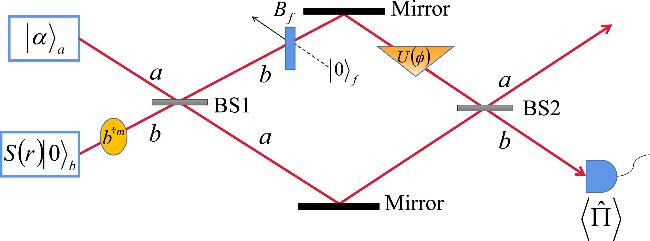
Figure 1. Schematic diagram of phase estimation with CS and PASVS inputting an MZI. In this configuration, photon loss within the MZI is simulated by a virtual beam splitter, and a parity detection scheme is employed at the output port. |
Our scheme aims to enhance the precision of phase measurement by utilizing CS and PASVS as input to the MZI. The input state is expressed as ${\left|\psi \right\rangle }_{{\rm{in}}}={\left|\alpha \right\rangle }_{a}\otimes {\left|r,m\right\rangle }_{b}$, where ${\left|\alpha \right\rangle }_{a}$ represents the CS at the a-mode input, and ${\left|r,m\right\rangle }_{b}$ denotes the PASVS at the b-mode input. The CS satisfies $a{\left|\alpha \right\rangle }_{a}=\alpha {\left|\alpha \right\rangle }_{a}$, where the amplitude parameter $\alpha =\left|\alpha \right|{{\rm{e}}}^{{\rm{i}}\theta }$. To simplify, we set θ = 0 ($\alpha =\left|\alpha \right|$), making it more advantageous for enhanced phase estimation [40, 50]. The state ${\left|r,m\right\rangle }_{b}$ is generated through non-Gaussian operations involving mth-order photon addition b†m to the SVS, defined as
$\begin{eqnarray}{\left|r,m\right\rangle }_{b}=\frac{1}{\sqrt{{P}_{m}}}{b}^{\dagger m}S\left(r\right){\left|0\right\rangle }_{b},\end{eqnarray}$
where Pm is the normalization factor, and $S\left(r\right)\,=\exp \left[r\left({b}^{2}-{b}^{\dagger 2}\right)/2\right]$ denotes the squeezing operator with the squeezing parameter r. In particular, when m = 0, this corresponds to that CS mixed with SVS is utilized as input. Using $S\left(r\right){\left|0\right\rangle }_{b}=$sech${}^{1/2}r\exp \left[-{b}^{\dagger 2}\tanh r/2\right]{\left|0\right\rangle }_{b}$ and ${b}^{\dagger m}\,=\frac{{\partial }^{m}}{\partial {\tau }^{m}}{\left.{{\rm{e}}}^{{b}^{\dagger }\tau }\right|}_{\tau =0}$ , ${\left|r,m\right\rangle }_{b}$ can be rewritten as $\begin{eqnarray}{\left|r,m\right\rangle }_{b}=\frac{{\left.\frac{{\partial }^{m}}{\partial {\tau }^{m}}\exp \left[{b}^{\dagger }\tau -\frac{1}{2}{b}^{\dagger 2}\tanh r\right]\right|}_{\tau =0}{\left|0\right\rangle }_{b}}{\sqrt{{P}_{m}\cosh r}},\end{eqnarray}$
thus, Pm and ${\bar{n}}_{b}$ can be derived as $\begin{eqnarray}\begin{array}{r}{P}_{m}={\left.\frac{{\partial }^{2m}}{\partial {t}^{m}\partial {\tau }^{m}}{{\rm{e}}}^{-\frac{\sinh 2r}{4}\left({t}^{2}+{\tau }^{2}\right)}{{\rm{e}}}^{t\tau {\cosh }^{2}r}\right|}_{t=\tau =0},\end{array}\end{eqnarray}$
$\begin{eqnarray}\begin{array}{r}{\bar{n}}_{b}={\,}_{b}\left\langle r,m\right|{b}^{\dagger }b{\left|r,m\right\rangle }_{b}=\frac{{P}_{m+1}}{{P}_{m}}-1.\end{array}\end{eqnarray}$
Here, the total average photon number $\bar{N}\,={\,}_{{\rm{in}}}\left\langle \psi \right|\left({a}^{\dagger }a+{b}^{\dagger }b\right){\left|\psi \right\rangle }_{{\rm{in}}}={\bar{n}}_{a}+{\bar{n}}_{b}$ with ${\bar{n}}_{a}={\alpha }^{2}$.Several studies have demonstrated that for specific path-symmetric state inputs to the MZI, the parity detection using photon-number-resolving detectors can achieve the phase sensitivity saturating the QCRB. In this case, the parity detection constitutes an optimal measurement scheme, leading to significant theoretical and experimental advancements [34–40, 47, 49–55]. In the model illustrated in figure 1, the parity detection is employed to measure the phase shift at the b-mode output port of the MZI, where the parity operator is defined as ${{\rm{\Pi }}}_{b}={\left(-1\right)}^{{b}^{\dagger }b}={{\rm{e}}}^{{\rm{i}}\pi {b}^{\dagger }b}$.
To investigate the actual measurements, we simulated photon loss in the b-mode of the MZI by introducing a virtual beam splitter between BS1 and the phase shifter. The corresponding transformation relation is
$\begin{eqnarray}{B}_{f}^{\dagger }\left(\begin{array}{c}b\\ {b}_{f}\end{array}\right){B}_{f}=\left(\begin{array}{cc}\sqrt{1-l} & \sqrt{l}\\ -\sqrt{l} & \sqrt{1-l}\end{array}\right)\left(\begin{array}{c}b\\ {b}_{f}\end{array}\right),\end{eqnarray}$
where bf is the photon annihilation operator of the dissipative mode in which the vacuum noise ${\left|0\right\rangle }_{f}$ is located, and Bf represents the equivalent operator of a virtual beam splitter with reflectivity corresponding to a photon loss rate l. Specifically, l = 0 and l = 1 correspond to a lossless scenario and complete absorption, respectively.To simplify the study of the parity detection scheme, we define an equivalent operator for parity detection that encompasses the entire lossy MZI, denoted as ${{\rm{\Pi }}}_{b}^{{\rm{loss}}}$, as follows: A .
$\begin{eqnarray}{{\rm{\Pi }}}_{b}^{{\rm{loss}}}={\,}_{f}\left\langle 0\right|{B}_{1}^{\dagger }{B}_{f}^{\dagger }{U}^{\dagger }\left(\phi \right){B}_{2}^{\dagger }{{\rm{\Pi }}}_{b}{B}_{2}U\left(\phi \right){B}_{f}{B}_{1}{\left|0\right\rangle }_{f}.\end{eqnarray}$
Using the normal ordering form of ${{\rm{\Pi }}}_{b}^{{\rm{loss}}}$, it is convenient to compute the average value $\left\langle {{\rm{\Pi }}}_{b}\right\rangle ={\,}_{{\rm{in}}}\left\langle \psi \right|{{\rm{\Pi }}}_{b}^{{\rm{loss}}}{\left|\psi \right\rangle }_{{\rm{in}}}$, which characterizes the signals of parity detection. The derivation procedure and specific expressions for the normal ordering form of ${{\rm{\Pi }}}_{b}^{{\rm{loss}}}$, as well as the average value $\left\langle {{\rm{\Pi }}}_{b}\right\rangle $, are provided in Appendix Using equation (A11 ), we can depict the average value$\left\langle {{\rm{\Pi }}}_{b}\right\rangle $ as a function of φ. Figure 2 illustrates $\left\langle {{\rm{\Pi }}}_{b}\right\rangle $ with φ for both the ideal (l = 0) and photon loss (l = 0.1) cases. The intuitive link between a narrower peak width and higher local phase sensitivity holds when comparing curves of similar shape, as is the case here. As shown in figure 2(a), with fixed α = 2 and r = 0.5, the central peak or trough of $\left\langle {{\rm{\Pi }}}_{b}\right\rangle $ at φ = 0 narrows as the addition photon number m increases. This indicates that increasing m can effectively enhance the phase resolution of the parity signal [35, 36, 38–40, 47, 49–51, 54]. In addition, as shown in figure 2(b), when α = 2 and the total average photon number is fixed at $\bar{N}=8$, the width of the central peak (or trough) remains largely consistent across different m. Furthermore, as illustrated in figure 2, photon loss results in a broader central peak or trough of $\left\langle {{\rm{\Pi }}}_{b}\right\rangle $ relative to the ideal scenario. This shows that photon loss degrades the phase resolution. Based on the comparison of the dashed lines representing photon loss in figure 2(a), it is evident that the central peak or trough narrows as m increases. Thus, even in the presence of photon loss, the phase resolution can be enhanced by photon addition operations, which implies that photon addition may improve the local phase sensitivity with parity detection.
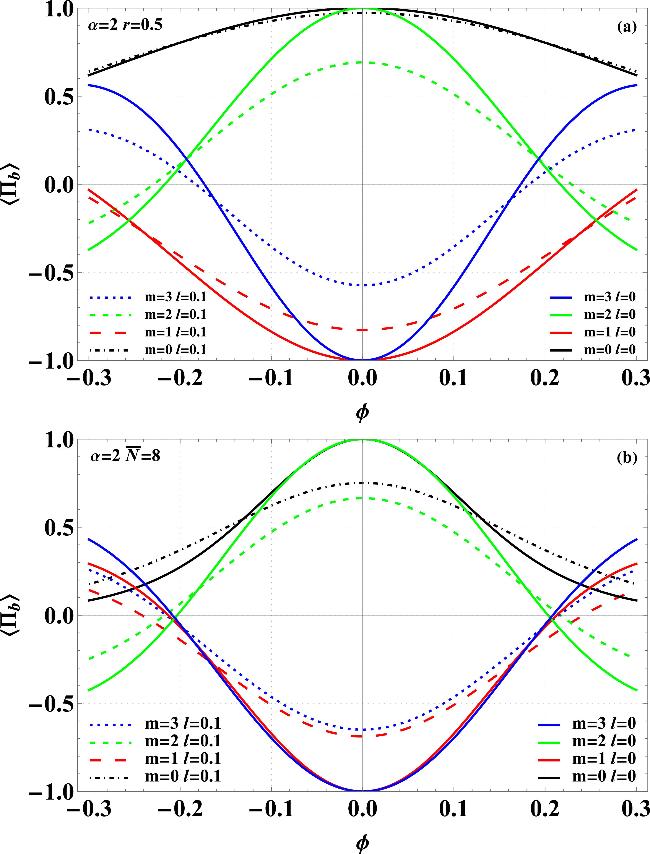
Figure 2. The variation of the parity signal ⟨Πb⟩ with phase shift φ for the ideal case (l = 0) and the photon loss case (l = 0.1), the addition photon number m = 0, 1, 2, 3 and the coherent amplitude α = 2, (a) with the fixed squeezing parameter r = 0.5, and (b) with the fixed total average photon number $\bar{N}=8$. |
3. Phase sensitivity with parity detection
In this section, we investigate the phase sensitivity of parity detection, also referred to as phase uncertainty, under both ideal and loss cases. Using the error propagation formula, we evaluate the phase sensitivity, i.e.A11 ) into equation (9 ), one can derive the phase sensitivity Δφ.
$\begin{eqnarray}{\rm{\Delta }}\phi =\frac{\sqrt{1-{\langle {{\rm{\Pi }}}_{b}\rangle }^{2}}}{\left|\partial \,\left\langle {{\rm{\Pi }}}_{b}\right\rangle /\partial \phi \right|}.\end{eqnarray}$
By substituting equation (Figure 3 illustrates the variation of the Δφ with the phase shift φ for both the ideal (l = 0) and photon loss (l = 0.1) cases. A smaller value of Δφ implies higher sensitivity and superior measurement precision. As shown in the figure 3, in the ideal case, Δφ reaches its optimum when φ = 0. Compared with the ideal scenario, photon loss degrades Δφ and causes the optimal point to deviate from φ = 0. As depicted in figure 3(a), when α = 2 and r = 0.5 are given, Δφ can be effectively decreased by increasing the addition photon number m within a certain range near the optimal point of φ. Furthermore, according to [40, 50, 56, 57], Δφ yields favorable results when ${\bar{n}}_{a}={\bar{n}}_{b}$ and $\bar{N}$ is fixed at a suitably large value. Thus, to further investigate the enhancement effect of our scheme on Δφ, figure 3(b) illustrates Δφ as a function of φ for α = 2 and $\bar{N}=8$ (${\bar{n}}_{a}={\bar{n}}_{b}=4$), and compares it with the SQL and the HL. It is shown that the ideal Δφ significantly surpasses the SQL and approaches the HL near the optimal point φ = 0. Moreover, near φ = 0, Δφ remains essentially the same for m = 0, 1, 2, 3 due to the energy constraint imposed by the fixed $\bar{N}$, while Δφ improves with increasing m within certain ranges away from φ = 0. However, as shown in the same figure, photon loss (l = 0.1) causes a general deterioration of Δφ and shifts the optimal phase point away from φ = 0. Nevertheless, even in the presence of loss, employing photon addition (m ≥ 1) yields better sensitivity than the case without addition (m = 0) over a broad phase range. However, by using the photon addition operations of m = 1, 2, 3, Δφ can be significantly improved relative to m = 0, and Δφ can still effectively break through the SQL within a certain range.
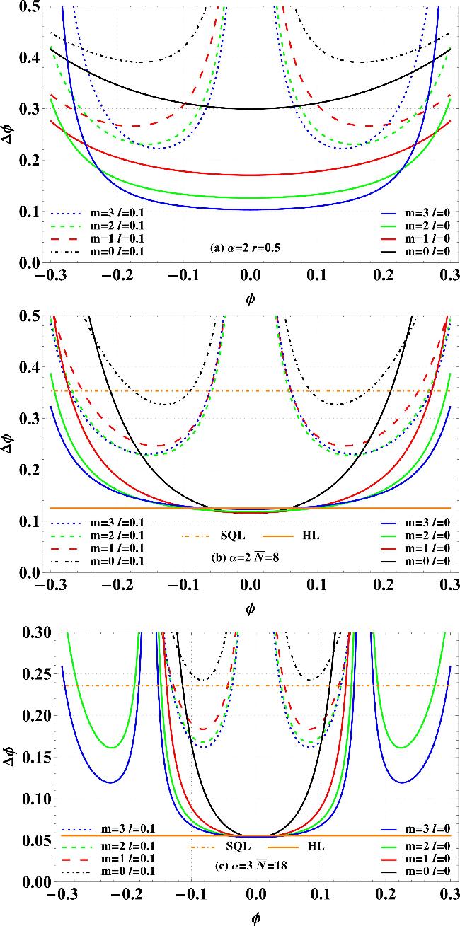
Figure 3. For the addition photon number of m = 0, 1, 2, 3, the phase sensitivity Δφ as a function of the phase shift φ for the ideal case (l = 0) and the photon loss case (l = 0.1). (a) With the fixed squeezing parameter r = 0.5 and the coherent amplitude α = 2, (b) with the fixed total average photon number $\bar{N}=8$ and α = 2, and (c) with the fixed $\bar{N}=18$ and α = 3. |
In experimental quantum optics, particularly in integrated photonic chips or superconducting circuit systems, the average number of photons is often constrained by practical limitations such as source intensity or detection efficiency, making operation in a low-photon-number regime common [58, 59]. Our choice of $\bar{N}=8$ for detailed analysis therefore represents a practical and relevant scenario within this constrained framework. However, the advantages of quantum metrology become more pronounced with a higher number of particles. Therefore, figure 3(c) shows Δφ versus φ curve when the average photon number $\bar{N}$ is fixed at a relatively high value of 18 (${\bar{n}}_{a}={\bar{n}}_{b}=9$ ). Similarly to figure 3(b), Δφ under ideal conditions can reach HL, and the photon addition operation can effectively enhance Δφ.
An interesting observation is that under ideal conditions (l = 0), the best sensitivity at φ = 0 is achieved for m = 0. As m increases, the sensitivity at φ = 0 slightly degrades, but improves significantly at adjacent phase values, broadening the high-sensitivity region. Furthermore, photon loss not only degrades the overall sensitivity but also shifts the optimal phase point. The photon-added states (m ≥ 1) demonstrate a clear advantage in mitigating the degradation caused by loss, especially away from the original optimal point.
As shown in figure 4, the phase sensitivity Δφ as a function of the squeezing parameter r and coherent amplitude α is depicted under both the ideal (l = 0) and photon loss (l = 0.1) scenarios. It is evident that the ideal Δφ can be enhanced by increasing r, α and the addition photon number m for a small phase shift φ = 10−4. Despite the impact of photon loss, when an appropriate φ = 0.15 is selected (as illustrated in figure 3, photon loss results in the optimal φ point deviating from 0), Δφ can still be significantly enhanced by increasing r, α and m within a certain range. Specifically, in figure 4(a), it is observed that under the photon loss, as m increases, the range over which Δφ improves with increasing r is confined to relatively small values of r. Actually, the smaller squeezing parameter r values are more experimentally feasible.
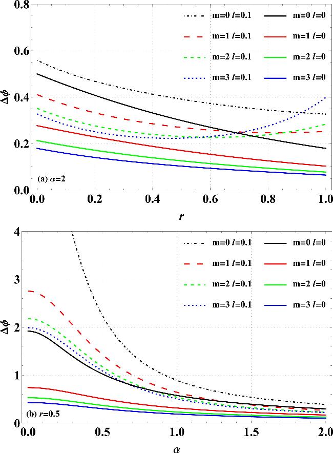
Figure 4. In the ideal case (l = 0) with fixed the phase shift φ = 10−4 and the photon loss case (l = 0.1) with fixed φ = 0.15, for the addition photon number m = 0, 1, 2, 3, (a) the phase sensitivity Δφ as a function of the squeezing parameter r with the coherent amplitude α = 2, (b) Δφ as a function of α with r = 0.5. |
To further analyze the influence of photon loss on phase sensitivity Δφ, as shown in figure 5, we present the variation of Δφ with respect to the loss rate l (phase shift φ is optimized). Although Δφ deteriorates with the increase of the loss rate l (see figure 5(a)), when α = 2 and r = 0.5 are fixed, Δφ can still be significantly improved by the photon addition operations of m = 1, 2, 3 within a certain range of relatively small l. Figure 5(b) shows Δφ versus l for α = 2 and $\bar{N}=8$, comparing the SQL and HL. It can be found that Δφ can reach the HL when l is very small, and in the case of photon loss, Δφ can still effectively break through the SQL in a certain range of l. Compared to the case of m = 0, Δφ of m = 1, 2, 3 has a significant improvement and can exceed the SQL in a larger range of l. Photon addition improves resilience against moderate losses (approximately when l < 0.3), particularly when the total photon number is constrained. However, for strong attenuation (approximately when l > 0.4), the fragility of non-Gaussian features dominates, diminishing the advantage.
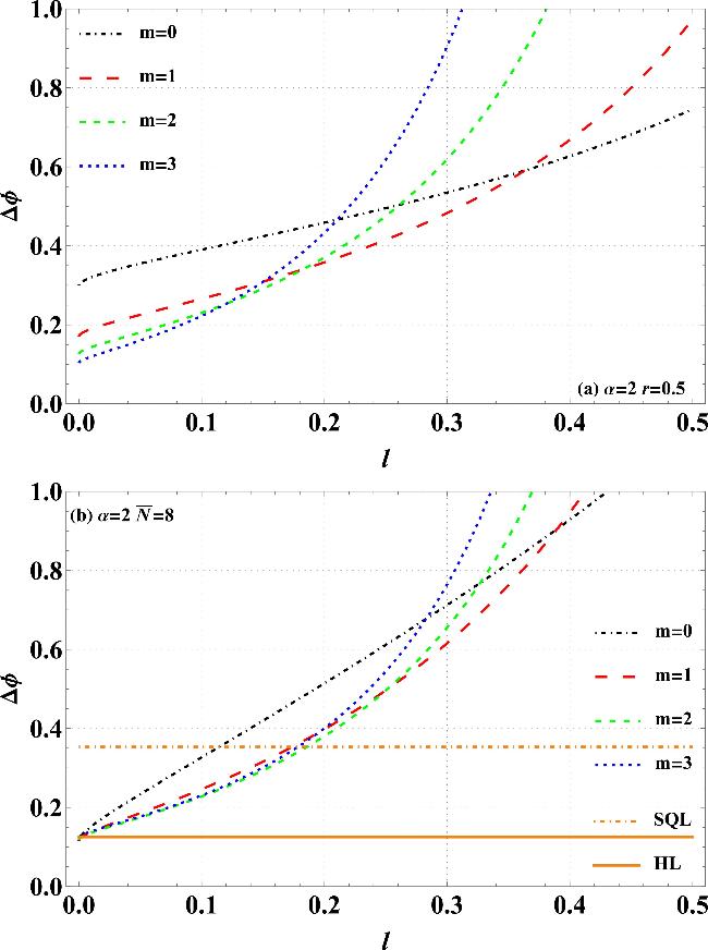
Figure 5. For the addition photon number m = 0, 1, 2, 3, the coherent amplitude α = 2, and optimized the phase shift φ, the phase sensitivity Δφ as a function of loss rate l (a) for given the squeezing parameter r = 0.5, and (b) for given the total average photon number $\bar{N}=8$, and compared with the SQL and the HL. |
4. The QFI in MZI
The QFI quantifies the maximum amount of obtainable information regarding the phase shift φ of a quantum system, independent of any detection scheme, and it is an upper bound of the CFI. The optimal error bound for phase sensitivity, known as the QCRB, is given by [60–62]
$\begin{eqnarray}{\rm{\Delta }}{\phi }_{{\rm{QCRB}}}=\frac{1}{\sqrt{{F}_{Q}}},\end{eqnarray}$
where FQ is the QFI. For a pure state, the QFI under ideal condition can be calculated as [63] $\begin{eqnarray}{F}_{Q}=4\left[\left\langle {\psi }_{\phi }^{{\prime} }| {\psi }_{\phi }^{{\prime} }\right\rangle -{\left|\left\langle {\psi }_{\phi }^{{\prime} }| {\psi }_{\phi }\right\rangle \right|}^{2}\right],\end{eqnarray}$
where $\left|{\psi }_{\phi }\right\rangle =U\left(\phi \right){B}_{1}{\left|\psi \right\rangle }_{{\rm{in}}}$ is the quantum state before BS2 in the lossless MZI, and $\left|{\psi }_{\phi }^{{}^{{\prime} }}\right\rangle =\partial \left|{\psi }_{\phi }\right\rangle /\partial \phi $. Thus, the QFI can be further simplified as $\begin{eqnarray}{F}_{Q}=4\left\langle {{\rm{\Delta }}}^{2}{n}_{b}\right\rangle =4\left[\left\langle {n}_{b}^{2}\right\rangle -{\left\langle {n}_{b}\right\rangle }^{2}\right],\end{eqnarray}$
where nb = b†b, and $\left\langle \cdot \right\rangle =\left\langle {{\rm{\Psi }}}_{S}\right|\cdot \left|{{\rm{\Psi }}}_{S}\right\rangle $, with $\left|{{\rm{\Psi }}}_{S}\right\rangle ={B}_{1}{\left|\psi \right\rangle }_{{\rm{in}}}$.For the initial pure state $\left|{{\rm{\Psi }}}_{S}\right\rangle $ in a probe system S with a lossy MZI, we introduce the orthogonal states $\left|{j}_{E}\right\rangle $ of the environment E and the Kraus operator ${\hat{{\rm{\Pi }}}}_{j}\left(\phi \right)$ to characterize the behavior of $\left|{{\rm{\Psi }}}_{S}\right\rangle $ as it passes through the phase shift. A diagram illustrating photon loss inside the MZI is provided in figure 6. According to Escher et al's methods for calculating QFI in open quantum systems [64], the quantum states $\left|{{\rm{\Psi }}}_{S}\right\rangle $ and the vacuum noise in the environment $\left|{0}_{E}\right\rangle $, after undergoing unitary evolution ${U}_{S+E}\left(\phi \right)$ that accounts for photon loss, can be expressed in the extended space of S + E as B3 ) (see Appendix B for details).
$\begin{eqnarray}\begin{array}{rc}\left|{{\rm{\Psi }}}_{S+E}\right\rangle & ={U}_{S+E}\left(\phi \right)\left|{{\rm{\Psi }}}_{S}\right\rangle \left|{0}_{E}\right\rangle \\ & =\displaystyle \sum _{j=0}^{\infty }{\hat{{\rm{\Pi }}}}_{j}\left(\phi \right)\left|{{\rm{\Psi }}}_{S}\right\rangle \left|{j}_{E}\right\rangle .\end{array}\end{eqnarray}$
Indeed, after photon loss, the quantum state $\left|{{\rm{\Psi }}}_{S}\right\rangle $ transitions into a mixed state; however, we treat the quantum state $\left|{{\rm{\Psi }}}_{S+E}\right\rangle $ in S + E as a pure state [64]. In this context, for the entire purified system, the QFI under photon loss can be expressed as $\begin{eqnarray}{F}_{Q}\leqslant {C}_{Q}\left[\left|{{\rm{\Psi }}}_{S}\right\rangle ,{\hat{{\rm{\Pi }}}}_{j}\left(\phi \right)\right]=4\left[\left\langle {\hat{H}}_{1}\right\rangle -{\left|\left\langle {\hat{H}}_{2}\right\rangle \right|}^{2}\right],\end{eqnarray}$
where the lower bound of ${C}_{Q}\left[\left|{{\rm{\Psi }}}_{S}\right\rangle ,{\hat{{\rm{\Pi }}}}_{j}\left(\phi \right)\right]$ is demonstrated to be the QFI for a reduced system [64], and ${\hat{H}}_{1,2}$ are Hermitian operators defined as $\begin{eqnarray}\begin{array}{rc}{\hat{H}}_{1} & =\displaystyle \sum _{j=0}^{\infty }\frac{{\rm{d}}{\hat{{\rm{\Pi }}}}_{j}^{\dagger }\left(\phi \right)}{{\rm{d}}\phi }\frac{{\rm{d}}{\hat{{\rm{\Pi }}}}_{j}\left(\phi \right)}{{\rm{d}}\phi },\end{array}\end{eqnarray}$
$\begin{eqnarray}\begin{array}{rc}{\hat{H}}_{2} & ={\rm{i}}\displaystyle \sum _{j=0}^{\infty }\frac{{\rm{d}}{\hat{{\rm{\Pi }}}}_{j}^{\dagger }\left(\phi \right)}{{\rm{d}}\phi }{\hat{{\rm{\Pi }}}}_{j}\left(\phi \right),\end{array}\end{eqnarray}$
where ${\hat{{\rm{\Pi }}}}_{j}\left(\phi \right)$ is the Kraus operator, i.e. $\begin{eqnarray}{\hat{{\rm{\Pi }}}}_{j}\left(\phi \right)=\sqrt{\frac{{l}^{j}}{j!}}{{\rm{e}}}^{{\rm{i}}\phi \left({b}^{\dagger }b-\gamma j\right)}{\left(1-l\right)}^{\frac{{b}^{\dagger }b}{2}}{b}^{j},\end{eqnarray}$
where γ = 0 or −1 correspond to photon loss before or after the linear phase shift, respectively. By optimizing γ, we can derive ${C}_{Q\min }$. Thus, the QFI in the presence of photon loss is obtained as [64] $\begin{eqnarray}{F}_{Q}=\frac{4\left(1-l\right)\left\langle {n}_{b}\right\rangle \left\langle {{\rm{\Delta }}}^{2}{n}_{b}\right\rangle }{l\left\langle {{\rm{\Delta }}}^{2}{n}_{b}\right\rangle +\left(1-l\right)\left\langle {n}_{b}\right\rangle },\end{eqnarray}$
where, $\left\langle {n}_{b}\right\rangle $ and $\left\langle {n}_{b}^{2}\right\rangle $ can be obtained by equation (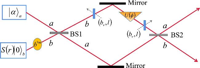
Figure 6. Theoretical model of lossy MZI using CS mixed with PASVS as input. Two virtual optical beam splitters, positioned before and after the phase shift, simulate photon loss. The parameter l represents the reflectivity, or loss rate, of the optical beam splitter, while bv denotes the vacuum operator. |
Figure 7 illustrates the variation of the QFI with respect to the input state parameters and the impact of photon loss (l = 0.1) on the QFI. It is clear that, although photon loss decreases the QFI FQ, increasing the squeezing parameter r, the coherent amplitude α, and the addition photon number m can effectively increase FQ, thereby improving the QCRB as indicated by equation (10 ) (${\rm{\Delta }}{\phi }_{{\rm{QCRB}}}=1/\sqrt{{F}_{Q}}$), in both the ideal and photon loss cases. Furthermore, figure 7 indicates that for a given average photon number $\bar{N}$, increasing m appears to be a highly effective strategy for enhancing the QFI, comparable to or exceeding the effect of increasing the squeezing or coherent amplitude under many parameter configurations. This highlights the potential of photon addition as a powerful operation for boosting metrological performance within a fixed resource budget. Thus, the proposed input scheme can effectively improve the precision of phase measurement.
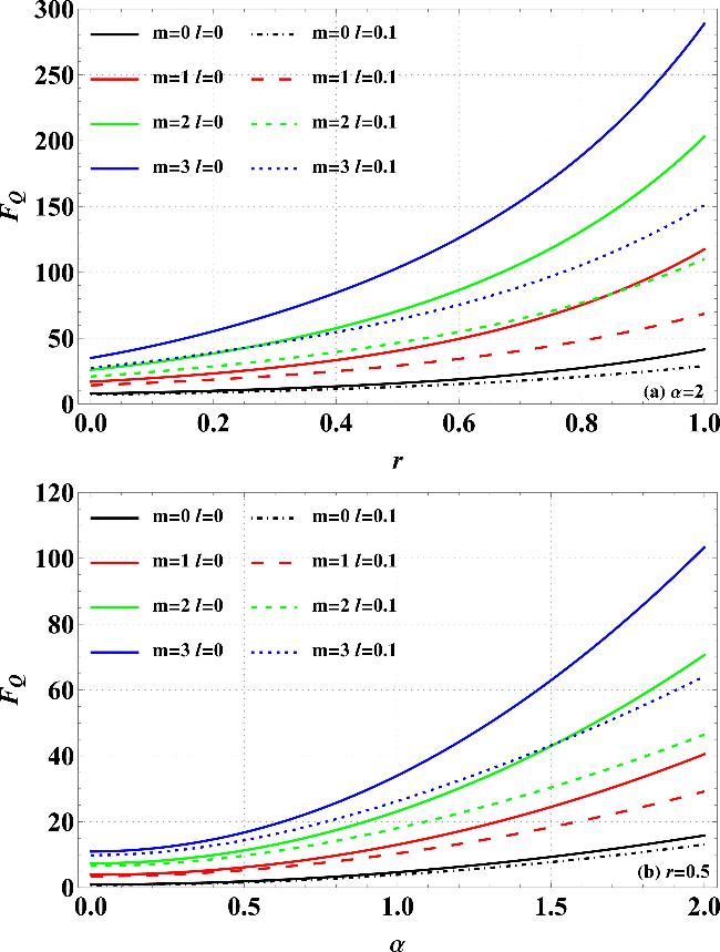
Figure 7. For the addition photon number m = 0, 1, 2, 3, in the ideal case of l = 0, and in the photon loss case of l = 0.1, (a) the variation of QFI FQ with the squeezing parameter r for given the coherent amplitude α = 2, and (b) the variation of FQ with α for given r = 0.5. |
In order to investigate the effect of photon loss on the QCRB ΔφQCRB, we plot the variation of ΔφQCRB with the loss rate l in figure 8. It can be found that ΔφQCRB deteriorates gradually as l increases. As can be seen in figure 8(a), ΔφQCRB can still be effectively improved by increasing m in the case of photon loss. This indicates that the robustness of the system to photon loss is significantly enhanced by using photon addition operations. In figure 8(b), it can be observed that ΔφQCRB can effectively surpass the SQL and even exceed the HL within a certain range of l, despite photon loss. Additionally, the ΔφQCRB is essentially the same for different m since $\bar{N}$ corresponding to the input resource energy is fixed.
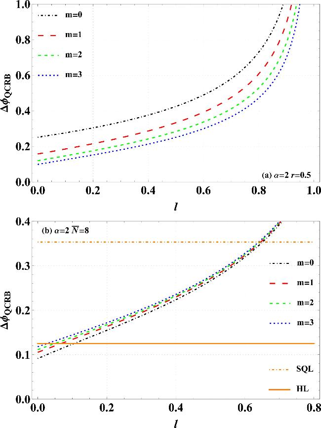
Figure 8. For the addition photon number m = 0, 1, 2, 3, and the coherent amplitude α = 2, the QCRB ΔφQCRB as a function of loss rate l, (a) for given the squeezing parameter r = 0.5, and (b) for given the total average photon number $\bar{N}=8$, and compared with the SQL and the HL. |
As shown in figure 9, the variation of the QCRB ΔφQCRB with respect to the total average photon number $\bar{N}$ is demonstrated and compared to the phase sensitivity Δφ as well as to the SQL and the HL. It can be clearly seen that for both the ideal (l = 0) and photon loss (l = 0.1) cases, ΔφQCRB and Δφ can be improved with the increase of $\bar{N}$ and m when the fixed squeezing parameter r = 0.5. As illustrated in figure 9(a), under ideal condition, ΔφQCRB and Δφ can evidently surpass the SQL and even approach the HL. Additionally, as m increases, Δφ progressively converges towards ΔφQCRB. Thus, in an ideal scenario, optimal measurement for CS mixed PASVS input MZI scheme can be achieved by employing parity detection. Figure 9(b) illustrates that despite photon loss, ΔφQCRB and Δφ can still effectively break through the SQL, and can be significantly improved by increasing $\bar{N}$ and utilizing photon addition operations.

Figure 9. The QCRB ΔφQCRB as a function of the total average photon number $\overline{N}$ for the addition photon number m = 0, 1, 2, 3, and fixed the squeezing parameter r = 0.5, (a) in the ideal case of l = 0, and (b) in the photon loss case of l = 0.1. The SQL, the HL and the variation of phase sensitivity Δφ with respect to $\overline{N}$ (for l = 0 and l = 0.1, fixed the phase shift φ = 10−4 and optimization φ, respectively) are also plotted for comparison. |
5. The QFI improved by Kerr nonlinear phase shift
Theoretically, the Kerr nonlinear transformation can substantially enhance measurement precision compared to the phase encoding process using linear transformation. Thus, this section further investigates the QFI replacing the linear phase shift $U\left(\phi \right)$ in the model of figure 6 with a Kerr nonlinear phase shift ${U}_{K}\left(\phi \right)$. Building upon prior research methodologies for the QFI with linear phase shift under both ideal and photon loss conditions, we further investigate the QFI in the Kerr nonlinear one. The Kerr nonlinear phase shift operator is defined as ${U}_{K}\left(\phi \right)=\exp \left[{\rm{i}}\phi {\left({b}^{\dagger }b\right)}^{2}\right]$, so according to equation (11 ) and substituting $\left|{\psi }_{\phi }\right\rangle ={U}_{K}\left(\phi \right){B}_{1}{\left|\psi \right\rangle }_{{\rm{in}}}$, the QFI for the Kerr nonlinear case under the ideal condition can be derived as B3 ) to obtain $\left\langle {n}_{b}^{2}\right\rangle $ and $\left\langle {n}_{b}^{4}\right\rangle $, and further substituting them into equation (19 ), the QFI for the ideal case of Kerr nonlinear phase shift can be obtained.
$\begin{eqnarray}{F}_{Q}=4\left\langle {{\rm{\Delta }}}^{2}{n}_{b}^{2}\right\rangle =4\left[\left\langle {n}_{b}^{4}\right\rangle -{\left\langle {n}_{b}^{2}\right\rangle }^{2}\right].\end{eqnarray}$
Substituting w = 2 and w = 4 into equation (Next, we investigate the QFI with photon loss for the Kerr nonlinear case. The general form of the Kraus operator, incorporating the Kerr nonlinear phase shift, is defined as follows [48]: 14 ), we derive (see Appendix C for derivation): C . To determine the QFI FQ under photon loss for the Kerr nonlinear case, we can substitute the optimal values of μ1 and μ2 (μ1opt and μ2opt) into CQ to find ${C}_{Q\min }$. The specific expressions of μ1opt and μ2opt are provided in Appendix C .
$\begin{eqnarray}{\hat{{\rm{\Pi }}}}_{j}\left(\phi \right)=\sqrt{\frac{{l}^{j}}{j!}}{{\rm{e}}}^{{\rm{i}}\phi \left[{\left({b}^{\dagger }b\right)}^{2}-2{\mu }_{1}{b}^{\dagger }bj-{\mu }_{2}{j}^{2}\right]}{\left(1-l\right)}^{\frac{{b}^{\dagger }b}{2}}{b}^{j},\end{eqnarray}$
where l is the loss rate, and the parameters μ1 = μ2 = 0 or −1 correspond to photon loss before or after the Kerr nonlinear phase shift. Referring to equation ( $\begin{eqnarray}\begin{array}{rcl}{F}_{Q} & \leqslant & {C}_{Q}\left[\left|{{\rm{\Psi }}}_{S}\right\rangle ,{\hat{{\rm{\Pi }}}}_{j}\left(\phi \right)\right]\\ & = & 4\left[{K}_{1}^{2}\left\langle {{\rm{\Delta }}}^{2}{n}_{b}^{2}\right\rangle -{K}_{2}\left\langle {n}_{b}^{3}\right\rangle +{K}_{3}\left\langle {n}_{b}^{2}\right\rangle \right.\\ & & \left.-{K}_{4}\left\langle {n}_{b}\right\rangle -{K}_{5}\left\langle {n}_{b}^{2}\right\rangle \left\langle {n}_{b}\right\rangle -{K}_{6}{\left\langle {n}_{b}\right\rangle }^{2}\right],\end{array}\end{eqnarray}$
where Ki (i = 1, 2, 3, 4, 5, 6) are detailed in Appendix Figure 10 illustrates the QFI FQ variation with the squeezing parameter r and coherent amplitude α for the Kerr nonlinear case, considering both ideal and photon loss scenarios. Clearly, FQ increases with r, α, and the addition photon number m. A comparison between figures 7 and 10 indicates that the QFI exhibits a substantial increase in the case of Kerr nonlinear case relative to the linear one. A comparison between figure 7 (linear) and figure 10 (Kerr) indicates that employing a Kerr nonlinear phase shift leads to a substantial increase in the QFI. This demonstrates that the combined use of photon addition operations and Kerr nonlinearity can effectively enhance the phase measurement precision beyond the linear scheme. Within the range of m considered, a higher photon addition order generally yields greater improvement.
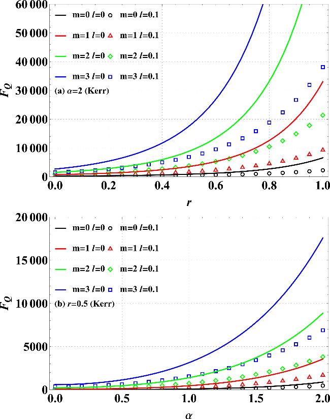
Figure 10. For the Kerr nonlinear phase shift case, and the addition photon number m = 0, 1, 2, 3, in the ideal case of l = 0 and in the photon loss case of l = 0.1, (a) the variation of QFI FQ with the squeezing parameter r for given the coherent amplitude α = 2, and (b) the variation of FQ with α for given r = 0.5. |
For the Kerr nonlinear case, the variation of QCRB ΔφQCRB with loss rate l is shown in figure 11. By comparing figure 11(a) with figure 8(a), a similar conclusion can be obtained, i.e. although photon loss worsens ΔφQCRB, the use of the photon addition operations remains effective in improving ΔφQCRB, and ΔφQCRB improves as m increases. ΔφQCRB of figure 11 has a significant improvement with respect to the linear phase shift case of figure 8. Moreover, it can be found from figure 11(b) that ΔφQCRB can break through the HL over a large range of l and can break through the sub-HL and even surpass the SHL over a certain range of l. This indicates that the utilization of the Kerr nonlinear phase shift can significantly improve the QCRB and the robustness against photon loss.
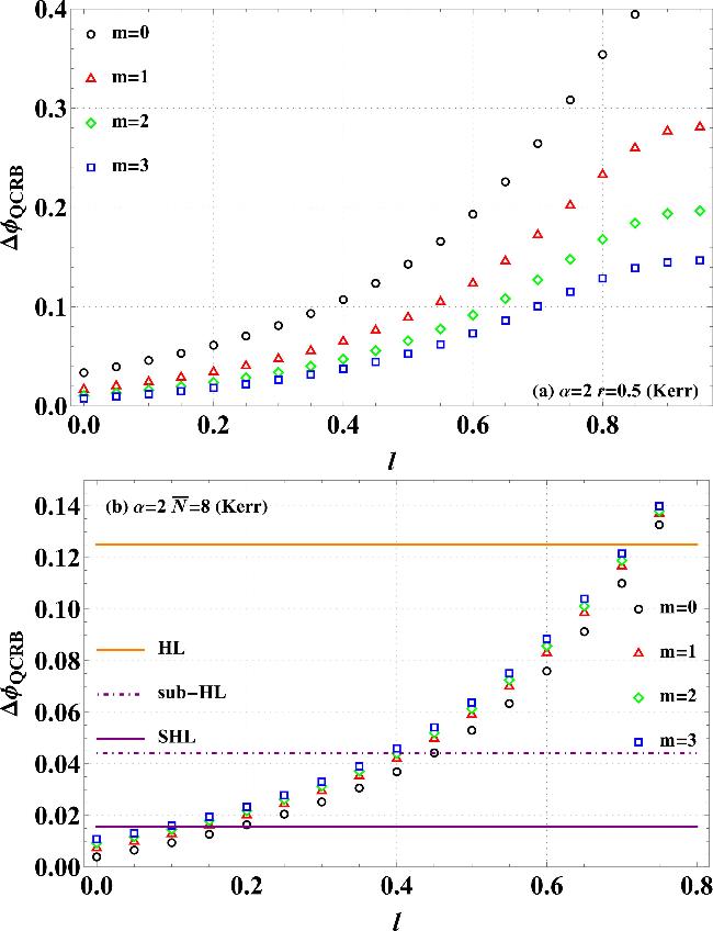
Figure 11. For the Kerr nonlinear phase shift case, the addition photon number m = 1, 2, 3, and the coherent amplitude α = 2, the QCRB ΔφQCRB as a function of loss rate l, (a) for given the squeezing parameter r = 0.5, and (b) for given the total average photon number $\bar{N}=8$, and compared with the SQL and the HL. |
To further reflect the improved effect of the Kerr nonlinear phase shift on the precision, figure 12 depicts the variation of the QCRB ΔφQCRB with respect to the total average photon number $\bar{N}$ and compares it with the HL, sub-HL, and SHL. It is clear from the figures that ΔφQCRB can be effectively improved for both the ideal (l = 0) and photon loss (l = 0.1) cases by increasing $\bar{N}$ and m. Furthermore, in the ideal case, ΔφQCRB of the Kerr nonlinear phase shift can break through the sub-HL to a large extent, and the photon addition operations of m = 1, 2, 3 can make ΔφQCRB approach or even exceed the SHL. In the case of l = 0.1, ΔφQCRB improved by the photon addition operations can still effectively break through the sub-HL. Thus, the utilization of both the photon addition operations and the Kerr nonlinear phase shift can further improve the measurement precision.
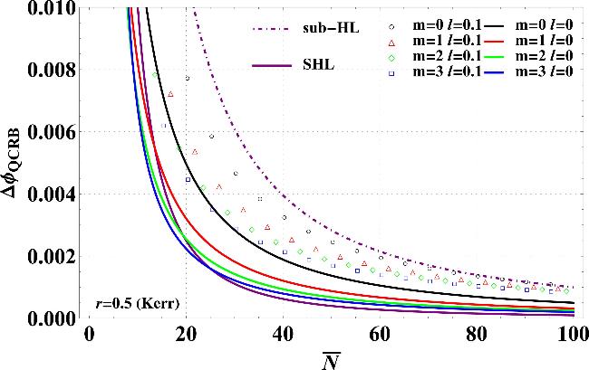
Figure 12. For the Kerr nonlinear phase shift case, the addition photon number m = 0, 1, 2, 3, and fixed the squeezing parameter r = 0.5, in the ideal case of l = 0 and in the photon loss case of l = 0.1, the variation of QCRB ΔφQCRB with respect to the total average photon number $\overline{N}$. The HL, sub-HL, and SHL are also plotted for comparison. |
6. Discussion
6.1. Two-phase QFI
In this paper, we primarily investigated the single-parameter QFI. However, in practical applications, when the two modes of the MZI exhibit different phase shifts, both the phase sum φ1 + φ2 and phase difference φ1 − φ2 become unknown and require simultaneous estimation. The single-parameter QFI is an overly optimistic estimate compared to the two-parameter QFI. To ensure the integrity and rigor of our work, we discuss the two-phase QFI here.
When considering phase shifts between the two paths of an MZI, the phase shift operator can be expressed as 23 ), the QCRB for the two-phase estimation can be derived, representing the lower bound of the estimation uncertainty [57, 65–67]:
$\begin{eqnarray}{U}_{\phi }={{\rm{e}}}^{{\rm{i}}{\phi }_{1}{a}^{\dagger }a}{{\rm{e}}}^{{\rm{i}}{\phi }_{2}{b}^{\dagger }b}={{\rm{e}}}^{{\rm{i}}{g}_{s}{\phi }_{s}}{{\rm{e}}}^{{\rm{i}}{g}_{d}{\phi }_{d}},\end{eqnarray}$
where ${g}_{s}=\left({a}^{\dagger }a+{b}^{\dagger }b\right)/2,{g}_{d}=\left({a}^{\dagger }a-{b}^{\dagger }b\right)/2$, and φ1, φ2 are the unknown phases on modes a and b, respectively. These phases can also be described using the phase sum φs = φ1 + φ2 and the phase difference φd = φ1 − φ2. For the estimation of φs and φd, the QFI matrix is given by $\begin{eqnarray}F=\left(\begin{array}{cc}{F}_{ss} & {F}_{sd}\\ {F}_{ds} & {F}_{dd}\end{array}\right),\end{eqnarray}$
where ${F}_{ij}=4\left(\left\langle {g}_{i}{g}_{j}\right\rangle -\left\langle {g}_{i}\right\rangle \left\langle {g}_{j}\right\rangle \right)$ and the subscrips s and d denote φs and φd, respectively. From equation ( $\begin{eqnarray}{\left|{\rm{\Delta }}\phi \right|}^{2}\geqslant {\left|{\rm{\Delta }}{\phi }_{{\rm{QCRB}}}\right|}^{2}=\,\rm{Tr}\,\left({F}^{-1}\right).\end{eqnarray}$
As shown in figure 13, the QCRB of the two-phase estimation improves with increasing squeezing parameter r and coherent amplitude α. Furthermore, increasing the addition photon number m significantly improves the QCRB, indicating that photon addition operations can effectively enhance measurement precision. This is consistent with the variation pattern of the QCRB with respect to the relevant parameters in the single-phase estimation scenario.
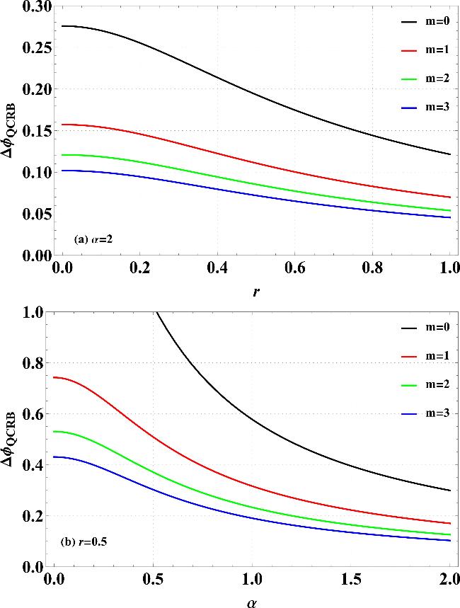
Figure 13. For the addition photon number m = 0, 1, 2, 3, (a) the variation of the two-phase QCRB ΔφQCRB with the squeezing parameter r for given the coherent amplitude α = 2, and (b) the variation of ΔφQCRB with α for given r = 0.5. |
When photon loss occurs in mode b, the entire system (interferometer + environment) undergoes a unitary evolution process ${U}_{{\rm{IE}}}\left({\phi }_{1},{\phi }_{2}\right)$, ultimately forming the global wave vector, 28 ) (see [66] for the detailed calculation process). As shown in figure 14, it is consistent with the variation law of single-phase estimation, although photon loss degrades the QCRB of the two-phase estimation, and the QCRB can be effectively improved through photon addition operations.
$\begin{eqnarray}\begin{array}{rcl}\left|{{\rm{\Psi }}}_{t}\right\rangle & = & {U}_{{\rm{IE}}}\left({\phi }_{1},{\phi }_{2}\right)\left|{{\rm{\Psi }}}_{S}\right\rangle \left|{0}_{E}\right\rangle \\ & = & \displaystyle \sum _{j=0}^{\infty }{\hat{{\rm{\Pi }}}}_{j}\left({\phi }_{1},{\phi }_{2}\right)\left|{{\rm{\Psi }}}_{S}\right\rangle \left|{j}_{E}\right\rangle ,\end{array}\end{eqnarray}$
where the Kraus operator ${\hat{{\rm{\Pi }}}}_{j}\left({\phi }_{1},{\phi }_{2}\right)$ can be expressed as $\begin{eqnarray}\begin{array}{rcl}{\hat{{\rm{\Pi }}}}_{j}\left({\phi }_{1},{\phi }_{2}\right) & = & \sqrt{\frac{{l}^{j}}{j!}}{{\rm{e}}}^{{\rm{i}}{\phi }_{d}\frac{{a}^{\dagger }a-{b}^{\dagger }b+{\gamma }_{2}j}{2}}\\ & & \times {{\rm{e}}}^{{\rm{i}}{\phi }_{s}\frac{{a}^{\dagger }a+{b}^{\dagger }b-{\gamma }_{2}j}{2}}{\left(1-l\right)}^{\frac{{b}^{\dagger }b}{2}}{b}^{j}.\end{array}\end{eqnarray}$
To obtain the two-phase QFI for photon loss conditions, the following matrix calculation can be utilized [68]: $\begin{eqnarray}C=\left(\begin{array}{cc}{C}_{ss} & {C}_{sd}\\ {C}_{ds} & {C}_{dd}\end{array}\right),\end{eqnarray}$
where the matrix elements Ckl ($k,l\in \left\{s,d\right\}$) can be obtained through the following expression: $\begin{eqnarray}{C}_{kl}=4\left(\left\langle \frac{\partial {{\rm{\Psi }}}_{t}}{\partial {\phi }_{k}}\right|{\left.\frac{\partial {{\rm{\Psi }}}_{t}}{\partial {\phi }_{l}}\right\rangle }^{2}-\left\langle \frac{\partial {{\rm{\Psi }}}_{t}}{\partial {\phi }_{k}}\right|\left.{{\rm{\Psi }}}_{t}\right\rangle \left\langle {{\rm{\Psi }}}_{t}\right.\left|\frac{\partial {{\rm{\Psi }}}_{t}}{\partial {\phi }_{l}}\right\rangle \right).\end{eqnarray}$
By optimizing γ2, a two-phase QFI under photon loss can be obtained, and the corresponding QCRB is derived from the inverse matrix of equation (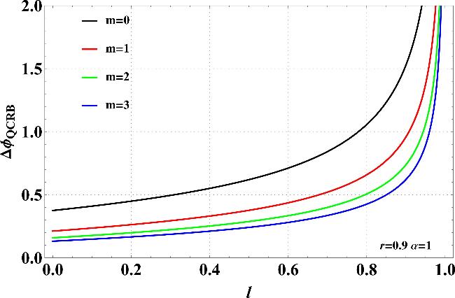
Figure 14. For the addition photon number m = 0, 1, 2, 3, the coherent amplitude α = 2, and the squeezing parameter r = 0.5, the two-phase QCRB ΔφQCRB as a function of loss rate l. |
6.2. Comparison of phase sensitivity and QCRB
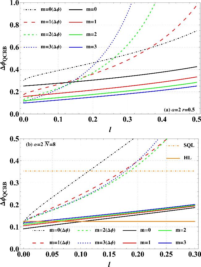
This subsection aims to discuss, through image comparisons, under what circumstances the phase sensitivity of parity detection can more closely approach the QCRB. As shown in figures 15(a) and (b), under ideal conditions, the phase sensitivity gradually saturates at the QCRB as the squeezing parameter r, coherent amplitude α, and addition photon number m increase. However, as shown in figures 15(c) and (d), when the photon loss rate l = 0.1 occurs, the degree of saturation of the phase sensitivity relative to the QCRB is significantly affected, meaning the phase sensitivity deviates considerably from the QCRB.
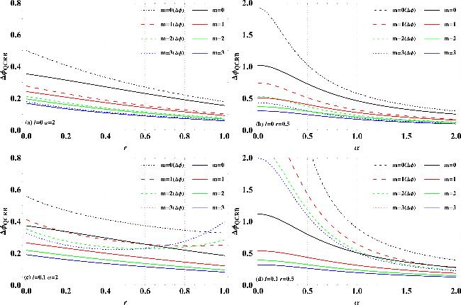
Figure 15. For the addition photon number m = 0, 1, 2, 3, in the ideal case of l = 0, (a) the QCRB ΔφQCRB and phase sensitivity Δφ as a function of the squeezing parameter r for given the coherent amplitude α = 2 and the phase shift φ = 10−4, (b) ΔφQCRB and Δφ as a function of α for given r = 0.5 and φ = 10−4; in the photon loss case of l = 0.1, (c) ΔφQCRB and Δφ as a function of r for given α = 2 and φ = 0.15, (d) ΔφQCRB and Δφ as a function of α for given r = 0.5 and φ = 0.15. |
In figure 16, (i) under the ideal case of l = 0, the phase sensitivity can approach the QCRB, at which point parity detection becomes the optimal measurement. (ii) However, under photon loss conditions, figure 16(b) reveals that the QCRB can surpass the SQL relative to phase sensitivity across a broader range of loss rates. (iii) The phase sensitivity deteriorates more rapidly with increasing loss rate compared to QCRB, suggesting that parity detection is relatively sensitive to photon loss.
Figure 16. For the addition photon number m = 0, 1, 2, 3, the coherent amplitude α = 2, and optimized the phase shift φ, the QCRB ΔφQCRB and phase sensitivity Δφ as a function of loss rate l, (a) for given the squeezing parameter r = 0.5, and (b) for given the total average photon number $\bar{N}=8$, and compared with the SQL and the HL. |
7. Conclusion
We propose a scheme that utilizes CS and PASVS inputs in an MZI to improve the precision of phase measurements. Our primary focus is on investigating the phase sensitivity with parity detection and the QFI, both under ideal conditions and in the presence of photon loss. The results indicate that the phase measurement precision is significantly improved by optimizing input resources, i.e. increasing the squeezing parameter r, coherent amplitude α, and total average photon number $\bar{N}$. Furthermore, the comparison reveals that the non-Gaussian operations of photon addition markedly enhance phase sensitivity and QFI. In the ideal case, the phase sensitivity and QCRB are improved with increasing the addition photon number m, significantly surpassing the SQL and even reaching the HL. In addition, the phase sensitivity can be better approximated to the QCRB by increasing m, which indicates that the parity detection is an optimal measurement for the phase estimation of the CS mixed PASVS inputs. In the presence of photon loss, the phase sensitivity and QCRB can still be significantly enhanced by increasing m, allowing the SQL to be surpassed across a relatively broad range of loss rates l.
In order to achieve a more effective improvement in measurement precision, we further considered replacing the linear phase shift in MZI with a Kerr nonlinear one. Based on the QFI for the Kerr nonlinear phase shift scenario, it is evident that both QFI and QCRB can be substantially enhanced in both the ideal case and the photon loss case by increasing the parameters r, α, and $\bar{N}$, as well as the photon addition operation m. Comparing the linear phase shift case, it is found that the Kerr nonlinear phase shift has a significant improvement on the QFI and QCRB, and the QCRB at photon loss can break through the HL over a wide range of the loss rate l, and can effectively exceed the sub-HL and even surpass the SHL over a certain range. In conclusion, our work demonstrates that the synergistic combination of non-Gaussian photon addition and Kerr nonlinear phase encoding provides a powerful route to enhance quantum phase estimation, offering both improved precision and increased robustness against photon loss. A valuable future direction would be a comprehensive study of phase estimation under asymmetric photon loss between the interferometer arms, which presents a more complex and practical scenario.
Appendix A The normal ordering of parity operator and its average value
To facilitate the computation of the normal ordering form of the equivalent operator for parity detection ${{\rm{\Pi }}}_{b}^{{\rm{loss}}}$ encompassing the entire lossy MZI, we first present the Weyl ordering form representation of the parity operator Πb in the ideal case [55, 69], as follows 8 ), by employing the invariance of Weyl ordering under similarity transformations [70] and combining the linear phase shift case with the operator transformation relation concerning the lossy MZI, we obtain 1 )–(2 ) and (7 )), we can derive
$\begin{eqnarray}{{\rm{\Pi }}}_{b}=\frac{\pi }{2}\,\begin{array}{c}:\\ :\end{array}\,\delta \left(b\right)\delta \left({b}^{\dagger }\right)\,\begin{array}{c}:\\ :\end{array}\,,\,\end{eqnarray}$
where$\,\begin{array}{c}:\\ :\end{array}\bullet \,\begin{array}{c}:\\ :\end{array}$ is the Weyl ordering and $\delta \left(\cdot \right)$ denotes the delta function. According to equation ( $\begin{eqnarray}\begin{array}{rcl}{{\rm{\Pi }}}_{b}^{{\rm{loss}}} & = & {\,}_{f}\left\langle 0\right|{U}_{{\rm{MZI}}}^{\dagger }{{\rm{\Pi }}}_{b}{U}_{{\rm{MZI}}}{\left|0\right\rangle }_{f}\\ & = & \frac{\pi }{2}{\,}_{f}\left\langle 0\right|{U}_{{\rm{MZI}}}^{\dagger }\begin{array}{c}:\\ :\end{array}\delta \left(b\right)\delta \left({b}^{\dagger }\right)\begin{array}{c}:\\ :\end{array}{U}_{{\rm{MZI}}}{\left|0\right\rangle }_{f}\\ & = & \frac{\pi }{2}{\,}_{f}\left\langle 0\right|\begin{array}{c}:\\ :\end{array}{U}_{{\rm{MZI}}}^{\dagger }\delta \left(b\right)\delta \left({b}^{\dagger }\right){U}_{{\rm{MZI}}}\begin{array}{c}:\\ :\end{array}{\left|0\right\rangle }_{f},\end{array}\end{eqnarray}$
where ${U}_{{\rm{MZI}}}={B}_{2}U\left(\phi \right){B}_{f}{B}_{1}$ represents the equivalent operator of lossy MZI, considering photon loss in the b-mode. By further utilizing the transformation relation of UMZI (substituting the transformation relation of $U\left(\phi \right)$ as well as equations ( $\begin{eqnarray}\begin{array}{rcl}{{\rm{\Pi }}}_{b}^{{\rm{loss}}} & = & \frac{\pi }{2}{\,}_{f}\left\langle 0\right|\begin{array}{c}:\\ :\end{array}\delta \left\{{x}_{1}a+{x}_{2}b+{x}_{3}{b}_{f}\right\}\\ & & \times \delta \left\{{x}_{1}^{* }{a}^{\dagger }+{x}_{2}^{* }{b}^{\dagger }+{x}_{3}^{* }{b}_{f}^{\dagger }\right\}\begin{array}{c}:\\ :\end{array}{\left|0\right\rangle }_{f},\end{array}\end{eqnarray}$
where $\begin{eqnarray}\begin{array}{rcl}{x}_{1} & = & \frac{{\rm{i}}}{2}\left(1-{{\rm{e}}}^{{\rm{i}}\phi }\sqrt{1-l}\right),\\ {x}_{2} & = & \frac{1}{2}\left(1+{{\rm{e}}}^{{\rm{i}}\phi }\sqrt{1-l}\right),\\ {x}_{3} & = & {{\rm{e}}}^{{\rm{i}}\phi }\sqrt{\frac{l}{2}}.\end{array}\end{eqnarray}$
By using the normal ordering form of the associated Wigner operator, i.e. $\begin{eqnarray}\begin{array}{rcl}{{\rm{\Delta }}}_{a}\left(\alpha \right) & = & \frac{1}{\pi }:\exp \left[-2\left(a-\alpha \right)\left({a}^{\dagger }-{\alpha }^{* }\right)\right]:,\\ {{\rm{\Delta }}}_{b}\left(\beta \right) & = & \frac{1}{\pi }:\exp \left[-2\left(b-\beta \right)\left({b}^{\dagger }-{\beta }^{* }\right)\right]:,\\ {{\rm{\Delta }}}_{{b}_{f}}\left({\gamma }_{f}\right) & = & \frac{1}{\pi }:\exp \left[-2\left({b}_{f}-{\gamma }_{f}\right)\left({b}_{f}^{\dagger }-{\gamma }_{f}^{* }\right)\right]:,\end{array}\end{eqnarray}$
the classical correspondence of the Weyl ordering operator can be obtained as follows [71] $\begin{eqnarray}\begin{array}{l}\begin{array}{c}:\\ :\end{array}\,\,f\left(a,{a}^{\dagger },b,{b}^{\dagger },{b}_{f},{b}_{f}^{\dagger }\right)\,\,\begin{array}{c}:\\ :\end{array}\\ =\,8\displaystyle \int {{\rm{d}}}^{2}\alpha {{\rm{d}}}^{2}\beta {{\rm{d}}}^{2}{\gamma }_{f}f\left(\alpha ,{\alpha }^{* },\beta ,{\beta }^{* },{\gamma }_{f},{\gamma }_{f}^{* }\right)\\ \times \,{{\rm{\Delta }}}_{a}\left(\alpha \right){{\rm{\Delta }}}_{b}\left(\beta \right){{\rm{\Delta }}}_{{b}_{f}}\left({\gamma }_{f}\right),\end{array}\end{eqnarray}$
and by combining the integration within an ordered product (IWOP) technique with the following integral formula $\begin{eqnarray}\int \frac{{{\rm{d}}}^{2}z}{\pi }{{\rm{e}}}^{\zeta {\left|z\right|}^{2}+\xi z+\eta {z}^{* }+f{z}^{2}+g{z}^{* 2}}=\frac{{{\rm{e}}}^{\frac{-\zeta \xi \eta +{\xi }^{2}g+{\eta }^{2}f}{{\zeta }^{2}-4fg}}}{\sqrt{{\zeta }^{2}-4fg}},\end{eqnarray}$
one can further obtain the normal ordering form of ${{\rm{\Pi }}}_{b}^{{\rm{loss}}}$ $\begin{eqnarray}{{\rm{\Pi }}}_{b}^{{\rm{loss}}}=:\exp \left[{X}_{1}{a}^{\dagger }a+{X}_{2}{b}^{\dagger }b+{X}_{3}{a}^{\dagger }b+{X}_{3}^{* }a{b}^{\dagger }\right]:,\end{eqnarray}$
where $\begin{eqnarray}\begin{array}{rcl}{X}_{1} & = & \frac{l-2}{2}+\sqrt{1-l}\cos \phi ,\\ {X}_{2} & = & \frac{l-2}{2}-\sqrt{1-l}\cos \phi ,\\ {X}_{3} & = & \frac{{\rm{i}}l}{2}-\sqrt{1-l}\sin \phi .\end{array}\end{eqnarray}$
To facilitate the use of the normal ordering of the parity operator ${{\rm{\Pi }}}_{b}^{{\rm{loss}}}$ and compute its average value, we employ the CS representation. The input state can be expressed as A8 ) and (A10 ) and referring to equation (A7 ), we can calculate the average value of the parity operator for under photon loss: A11 ) represents the average value of the parity operator in the ideal scenario.
$\begin{eqnarray}\begin{array}{rcl}{\left|\psi \right\rangle }_{{\rm{in}}} & = & {\left|\alpha \right\rangle }_{a}\displaystyle \otimes {\left|r,m\right\rangle }_{b}\\ & = & \frac{1}{\sqrt{{P}_{m}\cosh r}}\frac{{\partial }^{m}}{\partial {\tau }^{m}}\displaystyle \int \frac{{{\rm{d}}}^{2}\beta }{\pi }\\ & & \times {\left.\exp \left[-\frac{{\left|\beta \right|}^{2}}{2}+\tau {\beta }^{* }-\frac{\tanh r}{2}{\beta }^{* 2}\right]\right|}_{\tau =0}{\left|\alpha \right\rangle }_{a}{\left|\beta \right\rangle }_{b},\end{array}\end{eqnarray}$
where ${\left|\beta \right\rangle }_{b}$ is a CS used to represent the PASVS input on the b-mode. Using equations ( $\begin{eqnarray}\begin{array}{rcl}\left\langle {{\rm{\Pi }}}_{b}\right\rangle & = & {\,}_{{\rm{in}}}\left\langle \psi \right|{{\rm{\Pi }}}_{b}^{{\rm{loss}}}{\left|\psi \right\rangle }_{{\rm{in}}}\\ & = & \frac{\exp \left[{A}_{1}{\alpha }^{2}\right]}{{P}_{m}\sqrt{\bar{A}}\cosh r}\\ & & \times {\left.\frac{{\partial }^{2m}}{\partial {t}^{m}\partial {\tau }^{m}}\exp \left[\frac{{A}_{2}+{A}_{3}\alpha }{\bar{A}}\right]\right|}_{t=\tau =0},\end{array}\end{eqnarray}$
where $\begin{eqnarray}\begin{array}{rcl}\bar{A} & = & 1-{\tanh }^{2}r{\left(1+{X}_{2}\right)}^{2},\\ {A}_{1} & = & {X}_{1}+\frac{{\tanh }^{2}r\left(1+{X}_{2}\right){\left|{X}_{3}\right|}^{2}}{\bar{A}}-\frac{\tanh r}{2\bar{A}}\left({X}_{3}^{2}+{X}_{3}^{* 2}\right),\\ {A}_{2} & = & \left(1+{X}_{2}\right)t\tau -\frac{\tanh r}{2}{\left(1+{X}_{2}\right)}^{2}\left({t}^{2}+{\tau }^{2}\right),\\ {A}_{3} & = & {X}_{3}^{* }t+{X}_{3}\tau -\tanh r\left(1+{X}_{2}\right)\left({X}_{3}t+{X}_{3}^{* }\tau \right).\end{array}\end{eqnarray}$
In particular, for l = 0, the result of equation (Appendix B The normal ordering for operator identity and its average value
This appendix derives the average of ${n}_{b}^{w}$ with respect to $\left|{{\rm{\Psi }}}_{S}\right\rangle $ in order to obtain an expression for the simplicity of calculating the QFI. The normal ordering of ${n}_{b}^{w}$ is obtained via the operator identity: A10 )) and utilizing the transformation relation for BS1 (equation (1 )), the form of $\left|{{\rm{\Psi }}}_{S}\right\rangle $ in the CS representation is given by B1 ) and (B2 ) along with the IWOP technique and the integral formula equation (A7 ), we obtain
$\begin{eqnarray}\begin{array}{rcl}{n}_{b}^{w} & = & \frac{{\partial }^{w}}{\partial {x}^{w}}{\left.\exp \left[x{b}^{\dagger }b\right]\right|}_{x=0}\\ & = & \frac{{\partial }^{w}}{\partial {x}^{w}}{\left.\,:\,\exp \left[\left({{\rm{e}}}^{x}-1\right){b}^{\dagger }b\right]:\right|}_{x=0}.\end{array}\end{eqnarray}$
Based on the CS representation of ${\left|\psi \right\rangle }_{\mathrm{in}}$ (equation ( $\begin{eqnarray}\begin{array}{rcl}\left|{{\rm{\Psi }}}_{S}\right\rangle & = & \frac{1}{\sqrt{{P}_{m}\cosh r}}\frac{{\partial }^{m}}{\partial {\tau }^{m}}\displaystyle \int \frac{{{\rm{d}}}^{2}\beta }{\pi }\exp \left[-\frac{{\left|\beta \right|}^{2}}{2}+\tau {\beta }^{* }\right]\\ & & \times {\left.\exp \left[-\frac{\tanh r}{2}{\beta }^{* 2}\right]\right|}_{\tau =0}{\left|{\alpha }_{1}\right\rangle }_{a}{\left|{\beta }_{1}\right\rangle }_{b},\end{array}\end{eqnarray}$
where ${\alpha }_{1}=\left(\alpha -{\rm{i}}\beta \right)/\sqrt{2}$ and ${\beta }_{1}=\left(\beta -{\rm{i}}\alpha \right)/\sqrt{2}$. Using equations ( $\begin{eqnarray}\left\langle {n}_{b}^{w}\right\rangle ={D}_{m,w}\left\{{E}_{M}\right\},\end{eqnarray}$
where $\begin{eqnarray}{D}_{m,w}\left\{\cdot \right\}=\frac{1}{{P}_{m}\cosh r}\frac{{\partial }^{2m+w}}{\partial {t}^{m}\partial {\tau }^{m}\partial {x}^{w}}{\left.\left\{\cdot \right\}\right|}_{t=\tau =x=0},\end{eqnarray}$
and $\begin{eqnarray}\begin{array}{rcl}{E}_{M} & = & \frac{{M}_{1}}{\sqrt{{M}_{0}}}\exp \left[\frac{2{M}_{2}t-{M}_{2}^{2}\tanh r}{2{M}_{0}}\right]\\ & & \times \exp \left[-\frac{{\left(s+1\right)}^{2}{t}^{2}\tanh r}{2{M}_{0}}\right],\end{array}\end{eqnarray}$
as well as $\begin{eqnarray}\begin{array}{rcl}{M}_{0} & = & 1-{\left(s+1\right)}^{2}{\tanh }^{2}r,\\ {M}_{1} & = & \exp \left[s\alpha \left(\alpha +{\rm{i}}\tau +\frac{s\alpha \tanh r}{2}\right)\right],\\ {M}_{2} & = & -{\rm{i}}s\alpha +\left({{\rm{e}}}^{x}-s\right)\left(\tau -{\rm{i}}s\alpha \tanh r\right),\end{array}\end{eqnarray}$
where $s=\frac{1}{2}\left({{\rm{e}}}^{x}-1\right)$.Appendix C CQ For the kerr nonlinear phase shift case
Here, we derive CQ for the Kerr nonlinear phase shift and its specific expression to obtain the QFI FQ under photon loss condition. To compute CQ using equations (14 )–(16 ) and (20 ) according to the method in [48, 64], we first obtain the normal ordering form of ${\left(1-l\right)}^{{n}_{b}}{n}_{b}^{q}$ by utilizing the operator identity from equation (B1 ) as follows 15 ) and (16 ) to obtain the generalized equation about nb expressed in terms of the partial differential operator ${D}_{q,p}=\frac{{\partial }^{q+p}}{\partial {x}^{q}\partial {y}^{p}}{\left.\left[\cdot \right]\right|}_{x=y=0}$ as B1 ).
$\begin{eqnarray}\begin{array}{rcl}{\left(1-l\right)}^{{n}_{b}}{n}_{b}^{q} & = & {\eta }^{{n}_{b}}{n}_{b}^{q}\\ & = & \frac{{\partial }^{q}}{\partial {x}^{q}}{\left.\exp \left[{n}_{b}\mathrm{ln}\eta \right]\exp \left[{n}_{b}x\right]\right|}_{x=0}\\ & = & :{\left.\frac{{\partial }^{q}}{\partial {x}^{q}}{{\rm{e}}}^{\left(\eta {{\rm{e}}}^{x}-1\right){b}^{\dagger }b}\right|}_{x=0}:,\end{array}\end{eqnarray}$
where for simplicity, we have set η = 1 − l. Based on this equation and further utilizing the IWOP technique, the following summation can be computed for the operators Sq,p associated with the Hermitian operators H1,2 from equations ( $\begin{eqnarray}\begin{array}{rcl}{S}_{q,p} & = & \displaystyle \sum _{j=0}^{\infty }\frac{{\left(1-\eta \right)}^{j}}{j!}{j}^{p}{b}^{\dagger j}{\eta }^{{n}_{b}}{n}_{b}^{q}{b}^{j}\\ & = & \displaystyle \sum _{j=0}^{\infty }\frac{{\left(1-\eta \right)}^{j}}{j!}{j}^{p}:{\left.{\left({b}^{\dagger }b\right)}^{j}\frac{{\partial }^{q}}{\partial {x}^{q}}{{\rm{e}}}^{\left(\eta {{\rm{e}}}^{x}-1\right){b}^{\dagger }b}\right|}_{x=0}:\\ & = & :\displaystyle \sum _{j=0}^{\infty }\frac{{\left[\left(1-\eta \right){b}^{\dagger }b\right]}^{j}}{j!}\frac{{\partial }^{q+p}}{\partial {x}^{q}\partial {y}^{p}}{\left.{{\rm{e}}}^{\left(\eta {{\rm{e}}}^{x}-1\right){b}^{\dagger }b+yj}\right|}_{x=y=0}:\\ & = & :\frac{{\partial }^{q+p}}{\partial {x}^{q}\partial {y}^{p}}{\left.{{\rm{e}}}^{\left[\eta {{\rm{e}}}^{x}+\left(1-\eta \right){{\rm{e}}}^{y}-1\right]{b}^{\dagger }b}\right|}_{x=y=0}:\\ & = & \frac{{\partial }^{q+p}}{\partial {x}^{q}\partial {y}^{p}}{\left.{\left[\eta {{\rm{e}}}^{x}+\left(1-\eta \right){{\rm{e}}}^{y}\right]}^{{n}_{b}}\right|}_{x=y=0}.\end{array}\end{eqnarray}$
The final step in the above equation employs the operator identity from equation (According to equation (14 ), by substituting the Kraus operator for the Kerr nonlinear phase shift case (equation (20 )) into equations (15 ) and (16 ), and using equation (C2 ) one can further get C3 )–(C5 ), optimizing through ∂CQ/∂μ1 = ∂CQ/∂μ2 = 0 to find the minimum value of CQ gives C3 ), along with using equation (B3 ) for w = 1, 2, 3, 4, results in ${F}_{Q}={C}_{Q\min }$.
$\begin{eqnarray}\begin{array}{rcl}{C}_{Q} & = & 4[{K}_{1}^{2}\left\langle {{\rm{\Delta }}}^{2}{n}_{b}^{2}\right\rangle -{K}_{2}\left\langle {n}_{b}^{3}\right\rangle +{K}_{3}\left\langle {n}_{b}^{2}\right\rangle \\ & & -{K}_{4}\left\langle {n}_{b}\right\rangle -{K}_{5}\left\langle {n}_{b}^{2}\right\rangle \left\langle {n}_{b}\right\rangle -{K}_{6}{\left\langle {n}_{b}\right\rangle }^{2}],\end{array}\end{eqnarray}$
where $\begin{eqnarray}\begin{array}{rcl}{K}_{1} & = & {\omega }_{1}{\eta }^{2}-2{\omega }_{2}\eta -{\mu }_{2},\\ {K}_{2} & = & 2\eta \left[3{\omega }_{1}^{2}{\eta }^{3}-3{\omega }_{3}^{2}{\eta }^{2}-{\omega }_{4}\eta +{\omega }_{5}\right],\\ {K}_{3} & = & \eta \left[11{\omega }_{1}^{2}{\eta }^{3}-2{\omega }_{6}^{2}{\eta }^{2}+{\omega }_{7}\eta -4{\omega }_{1}{\omega }_{2}\right],\\ {K}_{4} & = & \eta {\omega }_{1}^{2}\left(6{\eta }^{3}-12{\eta }^{2}+7\eta -1\right),\\ {K}_{5} & = & 2\left(1-\eta \right)\eta {\omega }_{1}{K}_{1},\\ {K}_{6} & = & {\left(1-\eta \right)}^{2}{\eta }^{2}{\omega }_{1}^{2},\end{array}\end{eqnarray}$
and $\begin{eqnarray}\begin{array}{rcl}{\omega }_{1} & = & 1+2{\mu }_{1}-{\mu }_{2},\\ {\omega }_{2} & = & {\mu }_{1}-{\mu }_{2},\\ {\omega }_{3} & = & 1+2\left(3{\mu }_{1}-2{\mu }_{2}\right)+\left(2{\mu }_{1}-{\mu }_{2}\right)\left(4{\mu }_{1}-3{\mu }_{2}\right),\\ {\omega }_{4} & = & 7{\mu }_{2}-6{\mu }_{1}+24{\mu }_{1}{\mu }_{2}-14{\mu }_{1}^{2}-9{\mu }_{2}^{2},\\ {\omega }_{5} & = & {\mu }_{2}{\omega }_{1}-2{\omega }_{2}^{2},\\ {\omega }_{6} & = & 9+40{\mu }_{1}-22{\mu }_{2}+44{\mu }_{1}^{2}-48{\mu }_{1}{\mu }_{2}+13{\mu }_{2}^{2},\\ {\omega }_{7} & = & 7+40{\mu }_{1}-26{\mu }_{2}+52{\mu }_{1}^{2}-64{\mu }_{1}{\mu }_{2}+19{\mu }_{2}^{2},\end{array}\end{eqnarray}$
where parameters μ1 and μ2 are optimizable to describe the photon losses occurring before and after the phase shifter. In particular, μ1 = μ2 = 0 or −1 represents photon losses occurring before or after the phase shift, respectively. Using equations ( $\begin{eqnarray}\begin{array}{r}{\mu }_{1{\rm{opt}}}=\frac{{G}_{2}{G}_{5}-{G}_{3}{G}_{4}}{{G}_{1}{G}_{4}-2\eta {G}_{2}^{2}},\end{array}\end{eqnarray}$
$\begin{eqnarray}\begin{array}{r}{\mu }_{2{\rm{opt}}}=\frac{{G}_{1}{G}_{5}-2\eta {G}_{2}{G}_{3}}{{G}_{1}{G}_{4}-2\eta {G}_{2}^{2}},\end{array}\end{eqnarray}$
where $\begin{eqnarray}\begin{array}{rcl}{G}_{1} & = & 2\left[-\left(1-\eta \right)\eta \left(\left\langle {{\rm{\Delta }}}^{2}{n}_{b}^{2}\right\rangle +2\left\langle {n}_{b}^{2}\right\rangle \left\langle {n}_{b}\right\rangle -{\left\langle {n}_{b}\right\rangle }^{2}\right)\right.\\ & & -\left(6{\eta }^{2}-6\eta +1\right)\left(\left\langle {n}_{b}^{3}\right\rangle +\left\langle {n}_{b}\right\rangle \right)\\ & & \left.+\left(11{\eta }^{2}-11\eta +2\right)\left\langle {n}_{b}^{2}\right\rangle \right],\end{array}\end{eqnarray}$
$\begin{eqnarray}\begin{array}{rcl}{G}_{2} & = & {\left(1-\eta \right)}^{2}\left\langle {{\rm{\Delta }}}^{2}{n}_{b}^{2}\right\rangle +3\left(1-\eta \right)\left(2\eta -1\right)\left\langle {n}_{b}^{3}\right\rangle \\ & & +\left(11{\eta }^{2}-13\eta +3\right)\left\langle {n}_{b}^{2}\right\rangle -\left(6{\eta }^{2}-6\eta +1\right)\left\langle {n}_{b}\right\rangle \\ & & -\left(1-\eta \right)\left(2\eta -1\right)\left\langle {n}_{b}^{2}\right\rangle \left\langle {n}_{b}\right\rangle +\eta \left(1-\eta \right){\left\langle {n}_{b}\right\rangle }^{2},\end{array}\end{eqnarray}$
$\begin{eqnarray}\begin{array}{rcl}{G}_{3} & = & {\eta }^{2}\left\langle {{\rm{\Delta }}}^{2}{n}_{b}^{2}\right\rangle -3\eta \left(2\eta -1\right)\left\langle {n}_{b}^{3}\right\rangle \\ & & +\left(11{\eta }^{2}-9\eta +1\right)\left\langle {n}_{b}^{2}\right\rangle -\left(6{\eta }^{2}-6\eta +1\right)\left\langle {n}_{b}\right\rangle \\ & & +\eta \left(2\eta -1\right)\left\langle {n}_{b}^{2}\right\rangle \left\langle {n}_{b}\right\rangle +\eta \left(1-\eta \right){\left\langle {n}_{b}\right\rangle }^{2},\end{array}\end{eqnarray}$
$\begin{eqnarray}\begin{array}{rcl}{G}_{4} & = & -{\left(1-\eta \right)}^{3}\left\langle {{\rm{\Delta }}}^{2}{n}_{b}^{2}\right\rangle -6\eta {\left(1-\eta \right)}^{2}\left\langle {n}_{b}^{3}\right\rangle \\ & & -\eta \left(1-\eta \right)\left(11\eta -4\right)\left\langle {n}_{b}^{2}\right\rangle -\eta \left(6{\eta }^{2}-6\eta +1\right)\left\langle {n}_{b}\right\rangle \\ & & +2\eta {\left(1-\eta \right)}^{2}\left\langle {n}_{b}^{2}\right\rangle \left\langle {n}_{b}\right\rangle +{\eta }^{2}\left(1-\eta \right){\left\langle {n}_{b}\right\rangle }^{2},\end{array}\end{eqnarray}$
and $\begin{eqnarray}\begin{array}{rcl}{G}_{5} & = & \eta \left[-\eta \left(1-\eta \right)\left(\left\langle {{\rm{\Delta }}}^{2}{n}_{b}^{2}\right\rangle -{\left\langle {n}_{b}\right\rangle }^{2}\right)\right.\\ & & -\left(6{\eta }^{2}-6\eta +1\right)\left(\left\langle {n}_{b}^{3}\right\rangle +\left\langle {n}_{b}\right\rangle \right)\\ & & +\left(11{\eta }^{2}-11\eta +2\right)\left\langle {n}_{b}^{2}\right\rangle \\ & & \left.+\left(2{\eta }^{2}-2\eta +1\right)\left\langle {n}_{b}^{2}\right\rangle \left\langle {n}_{b}\right\rangle \right],\end{array}\end{eqnarray}$
and substituting these into equation (