


1. Introduction
Similarly to the periodic table, which provides a systematic way of understanding and predicting the element properties in chemistry, the chart of nuclides is of importance to nuclear physics and has become a powerful tool for visualizing and studying nuclear properties [1]. The modern nuclide chart consists of more than 2500 known nuclides (nevertheless, less than one third of theoretical predictions) [2–4]. So far, it has been revealed that the so-called ‘island' (namely, a region of the chart of nuclides where nuclei have prominent property on the nuclear map) or ‘archipelago' of islands may exist on the nuclide chart. For instance, some of them have been discovered or predicted, including the archipelago of islands of inversion [5, 6], the archipelago of islands of D3h point group symmetry [7], the island of superheavy stability, the island of tetrahedral Td (‘pyramid') symmetry [8] and the island of asymmetric fission [1]. In this project we focus specifically on one island of an archipelago of hexadecapole-deformation nuclei [3, 9].
As it is well known, the nucleus is a quantum many-body system governed by short-range strong interaction. The density distribution of a nucleus usually decreases to zero exponentially at the border of such a compact system, which helps to introduce the notions of nuclear surface and shape, and further, the one-body mean-field Hamiltonian. Here, using the language of multipole expansion of the nuclear surface with spherical hamornics [2, 10], one can describe the nuclear shape with a set of deformation parameters (corresponding to the collective coordinates in the space spanned by orthogonal spherical harmonics). The multipole deformations, e.g., the quadrupole and hexadecapole ones, are the quantities in this framework. Let us remind that, besides, there are other several parameterization methods of nuclear shape in the literature, such as Cassinian ovals [11], matched quadratic surfaces [12] and generalized Lawrence shapes [13–15]. Needless to say, one has to describe the nuclear shape with other parameters instead of ‘multipole' deformations in those cases.
It is worth noting that, comparing with the quadrupole (e.g., prolate, oblate and triaxial) and octupole (e.g., pear-shaped and tetrahedral) deformations, the hexadecapole deformation has received less detailed attention since the effects of the hexadecapole correlations in nuclear low-lying states are often overshadowed by large quadrupole correlation effects [16]. Indeed, the hexadecapole deformation is difficult to extract from experiment with good precision due to the small magnitude and big uncertainty [17, 18]. Nevertheless, it was still pointed out that the hexadecapole correlations are nonnegligible in many rare-earth [19–22] and actinide [23–25] nuclei. In the production of superheavy elements, it was illustrated, e.g., by the dinuclear system model, that the hexadecapole deformation could change significantly the structure of the driving potentials and the fusion probabilities for some reaction channels [26]. In recent years, the developments of related theories and experimental techniques seems to renew the research enthusiasm of hexadecapole deformation in nuclei. For instance, the hexadecapole deformation was revealed to affect the values of the neutrinoless double β decay matrix elements of open shell nuclei in [27]. In the hydrodynamic simulation of the relativistic heavy ion collider, it was confirmed the hexadecapole deformation plays an important role [28]. Based on quasi-elastic scattering, the hexadecapole deformation in the light-mass nucleus 24Mg was recently determined in experiment [17]. For a recent analysis of in fission calculations, hexadecapole deformation was found to be of importance for near-to-scission configurations [29]. By the coupled-channel calculations, hexadecapole deformations were determined for 74,76Kr from inelastic proton scattering cross sections [30]. The impact of hexadecapole deformations on the collective spectra of axially deformed nuclei was investigated using the IBM approach [16]. The emergence and stability of static hexadecapole deformations as well as the impact in the development of dynamic deformation due to collective motion considering quadrupole-hexadecapole coupling are very recently studied for a selected set of radium, thorium, uranium, and plutonium isotopes, using the Gogny Hartree–Fock-Bogoliubov and generator coordinate method frameworks [31].
In our previous study [9], including the rotational cases, it was found that the nuclear chart has an archipelago of, at least, seven islands of hexadecapole-deformation nuclei, agreeing with the theoretical calculations, e.g., by Möller et al [2, 3], at ground states. Focusing on different nuclear properties (e.g., nonaxial deformation degrees of freedom and binding energy), we have formally visited two of them, sitting in the A ≈ 150 and 230 mass regions with positive hexadecapole-deformation value [32, 33]. Using the similar theoretical methods, e.g., Potential-Energy-Surface (PES) and Total-Routhian-Surface (TRS) calculations, we have performed numerous calculations on nuclear structure properties, such as triaxial and octupole deformations, fission barriers and pathways, isomers and nuclear mass [34–36]. In this work, based on MM model [2, 37] and HFBC calculation [38, 39], we tend to probe nuclear structure properties on the island of nuclei with negative hexadecapole deformations in the A ≈ 180 mass region, primarily paying attention to the effects of different quadrupole and hexadecapole deformations on nuclear moment of inertia (MoI) and the comparison with the calculations based on a deformed rigid body. In combination with the recent publications with the inclusion of exotic deformations [40, 41], the prediction is given by a natural extension of the rigid calculations.
This paper is organized as follows: in section 2 , we present theoretical approaches, including the MM model and CHFB calculations. The shape parameterization and nuclear rigid-body approximation are also introduced. Calculated results for, such as single-particle levels, PESs, equilibrium deformations and MoIs, are illustrated and discussed in section 3 . In particular, the effects of the hexadecapole deformation are presented and analyzed. Our theoretical results provide the reasonable explanations (predictions) for the available (unknown) data in this region. Finally, a summary and some concluding remarks are given in section 4 .
2. Theoretical method
In this section, we briefly recall the general procedure of our adopted theoretical methods and provide the necessary references.
Based on the well known special functions of applied mathematics, the nuclear shape is defined in terms of the spherical harmonic multipole expansion of nuclear surface Σ [42],
$\begin{eqnarray}{\rm{\Sigma }}:R(\theta ,\phi )={r}_{0}{A}^{\frac{1}{3}}c(\alpha )\left[1+\displaystyle \sum _{\lambda }\displaystyle \sum _{\mu =-\lambda }^{+\lambda }{\alpha }_{\lambda \mu }{Y}_{\lambda \mu }(\theta ,\phi )\right],\end{eqnarray}$
where R(θ, φ), sometimes written as R(θ, φ, α), indicates the distance from the origin of the coordinate system to the point on the nuclear surface whose position is specified by the angles θ and φ; the function c(α) ensures the conservation of the nuclear volume and α denotes a set of deformation parameters {αλμ} with non-negative integer indices λ and μ limited by −λ ≤ μ ≤ + λ. Once a set of {αλμ} is given, the nuclear shape will be fixed. If considering the constant density distribution in a nucleus, one can calculate the nuclear MoI based on a rigid-body approximation. For instance, according to the default convention of spherical and Cartesian coordinate systems, the rigid-body (with a fixed shape) MoI Jrig. around x axis (here, we just care for the cranking around x axis) reads, $\begin{eqnarray}\begin{array}{l}\displaystyle \int ({y}^{2}+{z}^{2}){\rm{d}}m\\ \quad =\displaystyle \int [{(r{\rm{\sin }}\theta {\rm{\sin }}\varphi )}^{2}+{(r{\rm{\cos }}\theta )}^{2}]\rho {\rm{d}}v\\ \quad =\rho {\displaystyle \int }_{0}^{\pi }{\rm{d}}\theta {\displaystyle \int }_{0}^{2\pi }{\rm{d}}\varphi {\displaystyle \int }_{0}^{R(\theta ,\varphi )}({\rm{\sin }}\theta -{{\rm{\sin }}}^{3}\theta {{\rm{\cos }}}^{2}\varphi ){r}^{4}{\rm{d}}r\\ \quad =\frac{\rho }{5}{\displaystyle \int }_{0}^{\pi }{\rm{d}}\theta {\displaystyle \int }_{0}^{2\pi }{R}^{5}(\theta ,\varphi )({\rm{\sin }}\theta -{{\rm{\sin }}}^{3}\theta {{\rm{\cos }}}^{2}\varphi ){\rm{d}}\varphi \\ \quad ={\displaystyle \int }_{0}^{\pi }{\rm{d}}\theta {\displaystyle \int }_{0}^{2\pi }f(\theta ,\varphi ){\rm{d}}\varphi .\end{array}\end{eqnarray}$
The above expression can be numerically calculated by using the 32-point Gauss–Legendre quadrature, e.g., ${\sum }_{i}^{32}{\omega }_{i}{\sum }_{j}^{32}{\omega }_{j}f({\theta }_{i},{\varphi }_{j})$, where θi, φj and ωi,j are nodes and weights, respectively; f(θ, φ) is the integrand. Combining the above two equations, in principle, the rigid-body MoI for a nucleus with arbitrary shape can be obtained, extending the empirical calculation, e.g., in [43].Generally speaking, most of nuclei prefer to possess three symmetry planes x − y, y − z and x − z, corresponding to R(π/2 + θ, φ) = R(π/2 − θ, φ), R(θ, π/2 + φ) =R(θ, π/2 − φ) and R(θ, φ) = R(θ, − φ), respectively. In this case, only the even λ and even μ components remain in equation (1 ). Therefore, in the shape parametrization, we just consider the low-order quadrupole and hexadecapole deformation degrees of freedom, including nonaxial deformations [that is, α≡ (α20, α2±2, α40, α4±2, α4±4)]. After requesting the hexadecpole degrees of freedom to be functions of the scalars in the quadrupole tensor α2μ, one can reduce the number of independent coefficients to three, namely, β2, γ and β4, which obey the relationships [44, 45],
$\begin{eqnarray}\left\{\begin{array}{l}{\alpha }_{20}={\beta }_{2}\cos \gamma \\ {\alpha }_{22}={\alpha }_{2-2}=-\frac{1}{\sqrt{2}}{\beta }_{2}\sin \gamma \\ {\alpha }_{40}=\frac{1}{6}{\beta }_{4}(5{\cos }^{2}\gamma +1)\\ {\alpha }_{42}={\alpha }_{4-2}=-\frac{1}{12}\sqrt{30}{\beta }_{4}\sin 2\gamma \\ {\alpha }_{44}={\alpha }_{4-4}=\frac{1}{12}\sqrt{70}{\beta }_{4}{\sin }^{2}\gamma .\end{array}\right.\end{eqnarray}$
Note that, in the deformation space mentioned above, the quadrupole β2 and hexadecapole β4 deformations satisfy ${\beta }_{2}^{2}={\alpha }_{20}^{2}+2{\alpha }_{22}^{2}$ and ${\beta }_{4}^{2}={\alpha }_{40}^{2}+2{\alpha }_{42}^{2}+2{\alpha }_{44}^{2}$ since the total deformation βλ at order λ is defined by ${\beta }_{\lambda }^{2}\,={\sum }_{\mu =-\lambda }^{\mu =+\lambda }{\alpha }_{\lambda \mu }^{2}$ [28] and the deformation magnitude βλ can usually be extracted from the ground-state electric transition rate B(Eλ) via ${\beta }_{\lambda }=\frac{4\pi }{(2\lambda +1)Z{R}_{o}^{\lambda }}\sqrt{\frac{B(E\lambda )}{{e}^{2}}}$, see e.g., [44].For a given nucleus with a fixed shape and taking the realistic Woods–Saxon (WS) potential into account, we can write down its model Hamiltonian as follows, 6 ) due to the different radius parameter. The Coulumb potential for protons reads
$\begin{eqnarray}{\hat{H}}_{{\rm{WS}}}=\hat{T}+{\hat{V}}_{{\rm{cent}}}(\overrightarrow{r};\hat{\beta })+{\hat{V}}_{{\rm{so}}}(\overrightarrow{r},\overrightarrow{p},\overrightarrow{s};\hat{\beta })+{\hat{V}}_{{\rm{Coul}}}(\overrightarrow{r},\hat{\beta }),\end{eqnarray}$
where $\hat{T}$ denotes the nucleonic kinetic-energy operator (namely, $-\frac{{\hslash }^{2}}{2m}{{\rm{\nabla }}}^{2}$). The central WS potential ${\hat{V}}_{{\rm{cent}}}(\overrightarrow{r};\hat{\beta })$ reads, $\begin{eqnarray}{\hat{V}}_{{\rm{cent}}}(\overrightarrow{r},\hat{\beta })=\frac{{V}_{0}[1\pm \kappa (N-Z)/(N+Z)]}{1+{\rm{\exp }}[{{\rm{dist}}}_{{\rm{\Sigma }}}(\overrightarrow{r},\hat{\beta })/{a}_{0}]},\end{eqnarray}$
where the plus and minus signs hold for protons and neutrons, respectively and the parameter a0 denotes the diffuseness of the nuclear surface. The term ${{\rm{dist}}}_{{\rm{\Sigma }}}(\overrightarrow{r},\hat{\beta })$ represents the distance between the single-particle (nucleon) position point $\overrightarrow{r}$ and the nuclear surface Σ. The spin-orbit potential ${\hat{V}}_{{\rm{so}}}$ which can strongly affect the level order is defined by, $\begin{eqnarray}\begin{array}{r}\begin{array}{l}{\hat{V}}_{{\rm{so}}}(\overrightarrow{r},\overrightarrow{p},\overrightarrow{s};\hat{\beta })=-\lambda {\left[\frac{\hslash }{2mc}\right]}^{2}\\ \quad \times \left\{{\rm{\nabla }}\frac{{V}_{o}[1\pm \kappa (N-Z)/(N+Z)]}{1+{\rm{\exp }}[{{\rm{dist}}}_{\displaystyle \sum _{{\rm{so}}}}](\overrightarrow{r},\hat{\beta })}\right\}\times \overrightarrow{p}\cdot \overrightarrow{s},\end{array}\end{array}\end{eqnarray}$
where λ denotes the strength parameter of the effective spin-orbit force acting on individual nucleons. The new surface ∑so is different form the one in equation ( $\begin{eqnarray}\begin{array}{r}{\hat{V}}_{{\rm{Coul}}}(\overrightarrow{r};\hat{\beta })=\frac{Z-1}{4\pi {R}_{0}^{3}/3}e\displaystyle \int \frac{{{\rm{d}}}^{3}r}{| \overrightarrow{r}-\overrightarrow{{r}^{{\prime} }}| }.\end{array}\end{eqnarray}$
The time-independent (stationary) Schrödinger equation ${\hat{H}}_{{\rm{WS}}}{\psi }_{n}={e}_{n}{\psi }_{n}$, as an eigenvalue equation, is solved numerically since the analytic solutions do not exist.To solve the eigenvalue equation, the general computational method is to build a Hamiltonian matrix by adopting a set of orthonormal basis functions and to obtain the eigenvalues and eigenfunctions by diagonalization. The computing efficiency of matrix diagonalization generally decreases rapidly as the number of adopted bases increases. That is, the computation time to diagonalize a Hamiltonian matrix increases very quickly as the number of bases increases. In principle, the Hilbert space, formed by the orthonormal basis functions, on which the Hamiltonian matrix is calculated, usually has an infinite dimension. Though our main goal is to obtain the N lowest eigenstates {ψn} and their energy values {en} of the WS Hamiltonian operator, the number of bases needed to properly describe a nuclear system is usually rather large (e.g., relative to N). Efficient implementation of the Hamiltonian matrix diagonalization requires that the matrix elements can be computed as fast as possible and the calculated Hamiltonian matrix has a small number of non-diagonal terms In general, the former can be simplified by using the time reversal (resulting in the Kramers degeneracy) and spatial symmetries (e.g., the parity and signature are conserved), while the latter can be realized by adopting appropriate basis functions and symmetry properties as well.
In the present project, we compute the WS Hamiltonian matrix in terms of a set of orthogonal complete bases, namely, the eigenfunctions of the axially deformed harmonic oscillator potential in the cylindrical coordinate system (obviously, the spherical basis functions will not be good candidates for a deformed shape). The deformed basis function has the following form [42], 9 ), the harmonic oscillator potential is constrained to approach the deformed WS one as much as possible (equivalently, let the harmonic oscillator ellipsoid overlap with the given nuclear shape as much as possible). One can usually obtain them by solving the equation system
$\begin{eqnarray}| N{n}_{z}{\rm{\Lambda }}{\rm{\Omega }}\rangle \equiv | {n}_{\rho }{n}_{z}{\rm{\Lambda }}{\rm{\Sigma }}\rangle ={\psi }_{{n}_{\rho }}^{{\rm{\Lambda }}}(\rho ){\psi }_{{n}_{z}}(z){\psi }_{{\rm{\Lambda }}}(\varphi )\chi ({\rm{\Sigma }}),\end{eqnarray}$
where N = 2nρ + ∣Λ∣ + nz, Ω = Λ + Σ and $\begin{eqnarray}\left\{\begin{array}{lcl}{\psi }_{{n}_{\rho }}^{{\rm{\Lambda }}}(\rho ) & = & \frac{\sqrt{{n}_{\rho }!}}{\sqrt{({n}_{\rho }+| {\rm{\Lambda }}| )!}}{(2m{\omega }_{\rho }/\hslash )}^{1/2}\\ & & \times {{\rm{e}}}^{-\frac{\eta }{2}}{\eta }^{{\rm{\Lambda }}}{L}_{{n}_{\rho }}^{| {\rm{\Lambda }}| }(\eta ),\\ {\psi }_{{n}_{z}}(z) & = & \frac{1}{\sqrt{\sqrt{\pi }{2}^{{n}_{z}}{n}_{z}!}}{(2m{\omega }_{z}/\hslash )}^{1/4}\\ & & \times {{\rm{e}}}^{-\frac{{\xi }^{2}}{2}}{H}_{{n}_{z}}(\xi ),\\ {\psi }_{{\rm{\Lambda }}}(\varphi ) & = & \frac{1}{\sqrt{2\pi }}{{\rm{e}}}^{i{\rm{\Lambda }}\varphi },\end{array}\right.\end{eqnarray}$
and χ(Σ) represents the spin wave functions, cf e.g., section 3.1 in [42] for more details. To obtain the approximate parameters ωρ and ωz in equation ( $\begin{eqnarray}\left\{\begin{array}{l}{\omega }_{\rho }^{2}{\omega }_{z}={\omega }_{0}^{3}\\ {\omega }_{\rho }/{\omega }_{z}=\sqrt{\langle {\rho }^{2}\rangle /\langle {z}^{2}\rangle }.\end{array}\right.\end{eqnarray}$
The average values ⟨ρ2⟩ and ⟨z2⟩ can be calculated with the help of the definition of nuclear surface by the integrals (e.g., ⟨z2 ⟩ = ∫z2dm/∫dm). The oscillator constant ω0, which can be determined from the mean square radius of a sphere, depends on the nuclear mass number A and satisfies the relationship, e.g., $\hslash {\omega }_{0}\simeq \frac{5}{4}{\left(\frac{3}{2}\right)}^{1/2}\frac{{\hslash }^{2}}{m{r}_{0}^{2}}{A}^{1/3}=41{A}^{1/3}$ MeV, i.e., see equation (2.12) in [46]. By such a treatment, the harmonic oscillator basis functions may satisfy the condition that makes the Hamiltonian matrix to have fewer and smaller off-diagonal elements, greatly improving the computational efficiency.The model parameters of the Hamiltonian are usually obtained by the inverse problem theory or χ2-fitting procedure (e.g. fitting the experimental single-particle levels). The adopted WS potential parameters are taken from [45], as given below:
(i) Radius parameters:
r0(p) = r0(n) = r0−so(p) = r0−so(n) = 1.190 fm;
(ii) Central potential depth parameters:
V0 = 53.754 MeV, κ = 0.791;
(iii) Spin-orbit potential strength constants:
λ(p) = λ(n) = 29.494;
(iv) Diffuseness parameters:
a0(p) = a0(n) = a0−so(p) = a0−so(n) = 0.637 fm.
Such a parameter set can describe the charge radii (both magnitude and isospin dependence) and high-spin properties (e.g., MoI) in nuclei, especially in medium and heavy mass regions. During our calculation, the eigenfunctions with the principal quantum number N≤ 12 and 14 have been chosen as a basis for protons and neutrons, respectively. It is found that, by such a basis cutoff, the single-particle energies are sufficiently convergent with respect to a basis-space enlargement. Concerning the original code used for solving the Schrödinger equation in the cylindrical coordinate system, one can refer to [42]. In order to evaluate the mixing of wave functions due to the multipole interaction, the Moshinsky bracket, e.g., ⟨NljΩ∣NnzΛΩ⟩ will be convenient for transferring the WS wave functions expanded by the cylindrical HO basis functions into the spherical HO bases, see the details in [47]. We implant such a transformation code in this work. Let us remind that the notation ∣NljΩ⟩ is equivalent to ∣nljΩ⟩ due to the existence of the constraint relation N = 2(n − 1) + l [33].
Once the single-particle levels {en} are obtained, one can calculate the shell correction $\delta {E}_{{\rm{shell}}}(Z,N,\hat{\beta })$, which is usually the most important part in the MM model. We compute this term by using a phenomenological expression firstly proposed by Strutinsky, 12 ) was optimized by introducing a phenomenological p-order curvature-correction polynomial Pp(x) [48–51]. Then, the $\tilde{g}(e,\gamma ,p)$ expression will have the form
$\begin{eqnarray}\delta {E}_{{\rm{shell}}}(Z,N,\hat{\beta })=\sum 2{e}_{i}-\int e\tilde{g}(e){\rm{d}}e,\end{eqnarray}$
where ei denotes the calculated single-particle levels and $\tilde{g}(e)$ is the so-called smooth level density, which was early defined as, $\begin{eqnarray}\tilde{g}(e,\gamma )\equiv \frac{1}{\gamma \sqrt{\pi }}\displaystyle \sum _{i}{\rm{\exp }}\left[-\frac{{(e-{e}_{i})}^{2}}{{\gamma }^{2}}\right],\end{eqnarray}$
where γ indicates the smoothing parameter without much physical significance. Later, in order to eliminate any possibly strong γ-parameter dependence, the mathematical form in the right-side of equation ( $\begin{eqnarray}\tilde{g}(e,\gamma ,p)=\frac{1}{\gamma \sqrt{\pi }}\displaystyle \sum _{i=1}{P}_{p}\left(\frac{e-{e}_{i}}{\gamma }\right)\times {\rm{\exp }}\left[-\frac{{(e-{e}_{i})}^{2}}{{\gamma }^{2}}\right],\end{eqnarray}$
where the corrective polynomial Pp(x) can be expanded in terms of the Hermite or Laguerre polynomials. The corresponding coefficients of the expansion can be obtained by using the orthogonality properties of these polynomials and Strutinsky condition, i.e., cf. the Appendix in [52]. To a large extent, this method can be considered standard so far (one can see [53] for more details). The smooth density is calculated with a sixth-order Hermite polynomial and a smoothing range γ = 1.20ℏω0, where ℏω0 = 41/A1/3 MeV, indicating a satisfactory independence of the shell correction on the parameters γ and p [53]. Besides, there are also some other methods developed for the shell correction calculations, e.g., the semiclassical Wigner–Kirkwood expansion method [54] and the Green's function method [55].As it is known, the mean field cannot well cover the short-range components of the nucleon-nucleon interactions and the most dominating residual interaction is the pairing force in the mean-field theory. Indeed, during the nuclear structural calculations within the framework of the MM models, besides the shell correction, another important quantum corrections is the pairing-energy contribution. Up to now, as shown in [56], various variants of the pairing-energy contribution in the microscopic-energy calculations exist. For instance, several kinds of the phenomenological pairing energy expressions are widely adopted in the applications of the MM approach [56], such as the pairing correlation and pairing correction energies employing or not employing the particle number projection technique. In the present work, we calculate the the pairing correlation energy ${E}_{{\rm{pair}}}(Z,N,\hat{\beta })$ employing the approximately particle number projection technique, namely, the Lipkin–Nogami (LN) method [57, 58] which aims to minimize the expectation value of the Hamiltonian: 15 ), the pairing correlation Epair, defined as the difference between paired solution ${E}_{{\rm{LN}}}$ and no-pairing solution ${E}_{{\rm{LN}}}$(Δ = 0), will have the expression, 15 ). In fact, the so-called ‘shell correction' δEshell e.g., in [61] agrees with the summation δEshell and δEpair in the present equations (11 ) and (17 ). There is no doubt, one should pay special attention to the basic definiations (such as shell correction, pairing correlation and pairing correction) in the literature and they may be slightly different.
$\begin{eqnarray}\begin{array}{r}\hat{{ \mathcal H }}={\hat{H}}_{{\rm{WS}}}+{\hat{H}}_{{\rm{pair}}}-{\lambda }_{1}\hat{N}-{\lambda }_{2}{\hat{N}}^{2},\end{array}\end{eqnarray}$
where ${\hat{H}}_{{\rm{pair}}}$ indicates the pairing interaction Hamiltonian [59, 60]. By such a pairing treatment, not only the spurious pairing phase transition but also the particle number fluctuation encountered in the simpler BCS calculation can be avoided. In this method, the LN pairing energy for an even–even nuclear system at ‘paired solution' (pairing gap Δ ≠ 0) can be computed by [2, 57] $\begin{eqnarray}\begin{array}{rcl}{E}_{{\rm{LN}}} & = & \displaystyle \sum _{k}2{{v}_{k}}^{2}{e}_{k}-\frac{{{\rm{\Delta }}}^{2}}{G}-G\displaystyle \sum _{k}{{v}_{k}}^{4}\\ & & -4{\lambda }_{2}\displaystyle \sum _{k}{{u}_{k}}^{2}{{v}_{k}}^{2},\end{array}\end{eqnarray}$
where ${{v}_{k}}^{2}$, ek, Δ and λ2 represent the occupation probabilities, single-particle energies, pairing gap and number-fluctuation constant, respectively. At ‘no-pairing solution' (Δ = 0), one can give the corresponding partner expression as follows $\begin{eqnarray}\begin{array}{rc}{E}_{{\rm{LN}}}({\rm{\Delta }}=0) & =\displaystyle \sum _{k}2{e}_{k}-G\frac{N}{2}.\end{array}\end{eqnarray}$
Together with equation ( $\begin{eqnarray}\begin{array}{rcl}{E}_{{\rm{pair}}} & = & \displaystyle \sum _{k}2{{v}_{k}}^{2}{e}_{k}-\frac{{{\rm{\Delta }}}^{2}}{G}-G\displaystyle \sum _{k}{{v}_{k}}^{4}\\ & & -4{\lambda }_{2}\displaystyle \sum _{k}{{u}_{k}}^{2}{{v}_{k}}^{2}+G\frac{N}{2}-\displaystyle \sum _{k}2{e}_{k}.\end{array}\end{eqnarray}$
At this moment, let us clarify some confusing points for the general readers. In the literature, e.g., cf [61, 62], the quantum shell correction and pairing contribution are sometime merged as the ‘shell correction' δEshell defined by the difference ${E}_{{\rm{LN}}}-{\tilde{E}}_{{\rm{Strut}}}$ (e.g., see equation (1) in [61]). Here, the definition of E${}_{{LN}}$ includes the term $G\frac{N}{2}$, somewhat different with the expression in equation (Nuclear collective rotation can be accounted for by the one-dimensional cranking approximation, supposing that the nuclear system is constrained to rotate around a fixed axis (e.g. the x − axis with the largest MoI) at a given rotational frequency ω [63]. For instance, under rotation, the Hamiltonian, as seen in equation (14 ), will take the cranking form
$\begin{eqnarray}{\hat{H}}^{\omega }={\hat{H}}_{{\rm{WS}}}+{\hat{H}}_{{\rm{pair}}}-\omega {\hat{j}}_{x}-{\lambda }_{1}\hat{N}-{\lambda }_{2}{\hat{N}}^{2}.\end{eqnarray}$
The resulting cranking LN equation follows the form of the well known Hartree–Fock–Bogolyubov-like (HFB) equation which can be solved by using the HFB cranking (HFBC) method, see, e.g., [58, 63, 64] for a detailed description. The HFBC equations read, $\begin{eqnarray}\left\{\begin{array}{l}\displaystyle {\sum }_{\beta \gt 0}\left\{\left[({e}_{\alpha }-\lambda ){\delta }_{\alpha \beta }-\omega {({j}_{x})}_{\alpha \beta }-G{\rho }_{\bar{\alpha }\bar{\beta }}^{* }+4{\lambda }_{2}{\rho }_{\alpha \beta }\right]\right.\\ \left.\times {U}_{\beta k}-{\rm{\Delta }}{\delta }_{\alpha \beta }{V}_{\bar{\beta }k}\right\}={E}_{k}{U}_{\alpha k},\\ \displaystyle {\sum }_{\beta \gt 0}\left\{\left[({e}_{\alpha }-\lambda ){\delta }_{\alpha \beta }-\omega {({j}_{x})}_{\alpha \beta }-G{\rho }_{\alpha \beta }+4{\lambda }_{2}{\rho }_{\bar{\alpha }\bar{\beta }}^{* }\right]\right.\\ \left.\times {V}_{\bar{\beta }k}+{{\rm{\Delta }}}^{* }{\delta }_{\alpha \beta }{U}_{\beta k}\right\}={E}_{k}{V}_{\bar{\alpha }k},\end{array}\right.\end{eqnarray}$
where ${\rm{\Delta }}=G{\sum }_{\alpha \gt 0}\,{\kappa }_{\alpha \bar{\alpha }}$, λ = λ1 + 2λ2(N + 1), Ek = ϵk − λ2 and ϵk is the quasi-particle energy [58]. The density matrix and pairing tensor are denoted by ρ and κ, respectively. Needless to say, the symmetries of the rotating potential (for example, the signature and parity are conserved in the present deformation space) can simplify the calculations. After applying an iterative procedure, the HFBC equations can be self-consistently solved. That is, the eigenvectors (matrices U and V) and eigenvalues (quasi-particle Routhians {Ek}) will be obtained at each frequency ω and each grid point in the selected deformation space. In principle, one can calculate any physical quantities with the help of the eigenfunctions (namely, matrices U and V). For instance, the energy in the rotating framework can be given by $\begin{eqnarray}\begin{array}{rcl}{E}^{\omega } & = & {\rm{Tr}}(e-\omega {j}_{x})\rho -\frac{{{\rm{\Delta }}}^{2}}{G}-G\displaystyle {\sum }_{\alpha ,\beta \gt 0}{\rho }_{\alpha ,\beta }{\rho }_{\tilde{\alpha },\tilde{\beta }}\\ & & -2{\lambda }_{2}{\rm{Tr}}\rho (1-\rho ),\end{array}\end{eqnarray}$
and the total collective angular momentum can be obtained from, $\begin{eqnarray}\begin{array}{r}{I}_{x}=\displaystyle \sum _{\alpha ,\beta \gt 0}\langle \beta | {j}_{x}| \alpha \rangle {\rho }_{\alpha \beta }+\displaystyle \sum _{\alpha ,\beta \gt 0}\langle \bar{\beta }| {j}_{x}| \bar{\alpha }\rangle {\rho }_{\bar{\alpha }\bar{\beta }},\end{array}\end{eqnarray}$
where the signature basis is denoted by α (β) and $\bar{\alpha }$ ($\bar{\beta }$) for the opposite signature). Then, the energy due to rotation (e.g., used for TRS) and the theoretical MoI Ix/ω (e.g., usually used for comparing with experimental results) can be calculated. Note that the aligned angular momentum Ix is the total angular momentum I for an even–even nucleus but it is a continuous variable and not conserved since the operator ${\hat{j}}_{x}$ does not commute with the Hamiltonian in the present cranking model. Concerning this point, one can also understand from the classic mechanics that, in the Lagrangian, the single-particle potential function includes the generalized coordinates θ and φ (which are not ignorable or cyclic coordinates) and so that the angular momentum is not conserved.So far, the MM calculations generally include several standard steps, i.e., as summarized in [37, 38, 65], by which one can calculate the total energy or Routhian at each sampling deformation point. Then, the smoothly energy/Routhian surface can further be given with the help of the interpolation techniques, e.g., by a spline interpolation. Finally, some physical quantities and/or processes, such as the equilibrium deformations, shape co-existence, fission path, can be studied. In the present project, we focus on the MoIs and energy surfaces affected by the deformations, especially the hexadecapole one.
3. Results and discussion
Let us start the presentation by visually illustrating the nuclear shapes with different quadrupole deformations and hexadecapole deformations involved in the present investigation. Figure 1 illustrates the shapes for α2μ=0,2 with arbitrarily selected values ± 0.3. One can see that the shapes with positive and negative α20 respectively correspond to prolate and oblate shapes, breaking the spherical symmetry and prolongating along the Z axis; and the positive and negative α22 values will respectively mean that the shape is compressed along the direction of Y and X axes, corresponding to the breaking of axial symmetry around Z axis. Similarly, the shapes with α4μ=0,2,4 = ± 0.3 are respectively displayed in figure 2. For the shape with α40, different signs correspond to different space distribution but other two hexadecapole deformations just have different orientations. Note that the relations between the collective coordinates αλμ and Bohr deformation parameters β2 and γ, cf e.g., equation (3 ). One can easily understand that the nucleus with the same shapes but different space orientations will obviously have the same mean-field potential, corresponding to the same model Hamiltonian and, certainly, the same single-particle levels. Practically, in the present calculations, nuclear shapes are usually the combination of these separated shapes exhibited in figures 1 and 2. The detailed description of nuclear shape and its symmetry properties should follow the expression mentioned in equation (1 ).
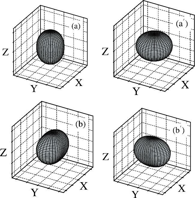
Figure 1. Illustrations of nuclear surfaces, defined by equation ( |
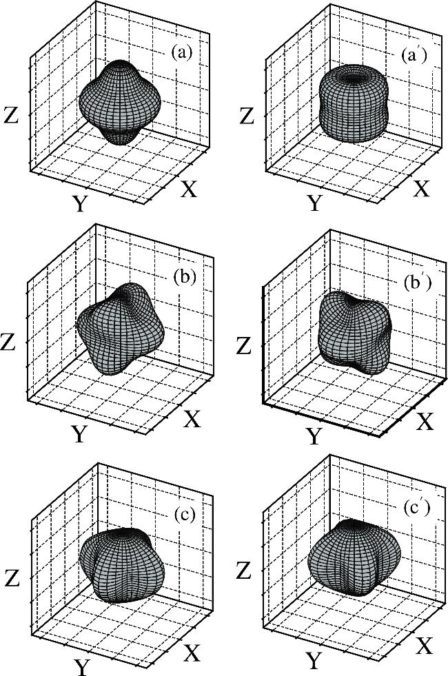
Figure 2. Similar to figure 1 but for α4μ = + 0.3 (left) and −0.3 (right), μ = 0 (a and a$^{\prime} $), 2 (b and b$^{\prime} $), 4 (c and c$^{\prime} $). |
As described in section 1 , the hexadecapole deformation is still important in nuclear physics and attracts experimental and theoretical attention [17, 28, 29]. Within the framework of MM models, by using the PES method—an important tool for studying the structural properties of atomic nuclei, we perform the energy surface calculations in the selected deformation spaces (β2, γ, β4), and (α20, α4μ=0,2,4) for probing the different hexadecapole deformation effects. Taking the central nucleus ${}_{72}^{184}$Hf112 as an example, the typical PESs are shown in figures 3 and 4. The calculated domains for the selected deformation space can be seen from the projected maps and the typical step is 0.05, except for Δγ = 5∘. Using the frequently-used Bohr deformation parameters, figure 3 illustrates three energy maps projected on (β2, γ), (β4, γ) and (β2, β4) planes. In each plane, the energy is minimized over the remaining deformation degrees of freedom, e.g. minimized over β4 in the (β2, γ) plane. Let us remind that in figure 3, the three minima in subfigures (a), (b) and (c) have the same energy and equilibrium shape. One can see that the triaxial γ is zero and β2 and β4 deformations are obviously nonzero, agreeing with the theoretical values given by Möller et al [3] (experimental data is scarce in this nucleus). Similarly, figure 4 presents the energy projections on the (α20, α4μ=0,2,4) planes. It is found that the axial hexadecapole deformation α40 has a relatively large value, ∼0.1, but the nonaxial α4μ=2,4 deformations are weak though the α42 value seems to nonzero. Furthermore, the energy minimum (∼−5.44 MeV) in figure 4(a) is about 2.5 MeV lower than, e.g., the minimum (∼−2.94 MeV) in figure 4(c), indicating that the α40 deformation may cause a large reduction in energy.
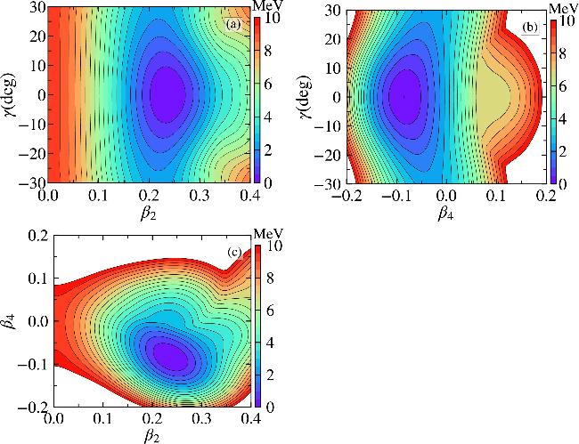
Figure 3. Projections of total energy on the (β2, γ) (a), (β4, γ) (b) and (β2, β4) (c) planes with contour-line separations of 0.5 MeV, minimized respectively at each deformation point over the remaining deformation, β4, β2 and γ, for the central nucleus 184Hf. Note that, for each subfigure, the energy normalization is specified by setting the minimum to zero at the equilibrium shape. In addition, the spline interpolation technique and the marching square algorithm are respectively adopted during the minimization and contouring processes. See the text for more details. |
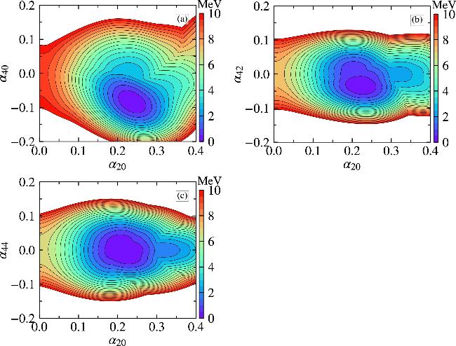
Figure 4. Similar to the preceding illustration in figure 3, but projected on the (α20, α4μ=0,2,4) planes for 184Hf. |
To verify the effectiveness of the present calculation, e.g., the adopted StkI parameters [45, 66–68], it might be necessary to confront with experimental observations or other theoretical results. We show the calculated equilibrium deformations β2 and β4 for present nine even–even nuclei on the selected hexadecapole deformation island in table 1, together with the theoretical results from the fold-Yukawa single-particle potential and the finite-range droplet model (FY+FRDM) [2], Hartree–Fock-BCS (HFBCS) [69] and the extended Thomas-Fermi plus Strutinsky integral (ETFSI) models [70], as well as partial experimental (Exp.) values of β2 [71] for comparison. From this table, it can be seen that all theoretical results, including phenomenological and self-consistent mean-field calculations, are somewhat smaller than the experimental data. However, according to the presently calculated results, one can see, as expected, that for each isotopic chain the quadrupole deformation β2 decreases as the neutron number N changes from 110 to 114, more and more approaching the magic number 126 from the mid-magic number 104; along each isotonic chain, β2 decreases as the proton number Z changes from 70 to 74, more and more approaching the magic number 82 from the mid-magic number 66. This trend is in good agreement with the available data (e.g., see the β2 evolution in even–even isotopes 184−188W) and also with those of the theoretical calculations in [2, 70], especially in [2] which also adopts the MM theoretical framework. The HFBC calculation seems to deviate from this general trend, particularly giving the oblate shape in 188W. As can be seen from the table 1, it can be concluded that the calculated results are model-dependent and no one can entirely agree with data. Nevertheless, all the theoretical calculations indicate the nonnegligible negative hexadecapole deformation β4 though the magnitudes are somewhat different.
Table 1. Calculated ground-state equilibrium deformations β2 and β4 for even–even nuclei 180−184Yb, 182−184Hf and 184−188W in the present work, together with the theoretical results by the FY+FRDM [2], HFBCS [69] and ETFSI [70] calculations and part of experimental (Exp.) β2 values [71] for comparison. All the calculated equilibrium γ deformations are almost zero and ignored here. See text for more explanations. |
| Nuclei | β2 | β4 | |||||||
|---|---|---|---|---|---|---|---|---|---|
| Present | FY+FRDM | HFBCS | ETFSI | Exp. | Present | FY+FRDM | HFBCS | ETFSI | |
| ${}_{70}^{180}$Yb110 | 0.267 | 0.250 | 0.260 | 0.310 | — | −0.071 | −0.084 | −0.05 | −0.08 |
| ${}_{70}^{182}$Yb112 | 0.257 | 0.242 | 0.270 | 0.290 | — | −0.087 | −0.101 | −0.06 | −0.07 |
| ${}_{70}^{184}$Yb114 | 0.240 | 0.233 | 0.240 | 0.280 | — | −0.084 | −0.104 | −0.05 | −0.09 |
| ${}_{72}^{182}$Hf110 | 0.249 | 0.268 | 0.240 | 0.280 | 0.274 | −0.079 | −0.099 | −0.05 | −0.06 |
| ${}_{72}^{184}$Hf112 | 0.237 | 0.256 | 0.250 | 0.260 | — | −0.087 | −0.114 | −0.05 | −0.08 |
| ${}_{72}^{186}$Hf114 | 0.220 | 0.225 | 0.220 | 0.250 | — | −0.087 | −0.119 | −0.05 | −0.07 |
| ${}_{74}^{184}$W110 | 0.221 | 0.232 | 0.240 | 0.250 | 0.234 | −0.070 | −0.093 | −0.05 | −0.07 |
| ${}_{74}^{186}$W112 | 0.210 | 0.221 | 0.210 | 0.250 | 0.227 | −0.077 | −0.095 | −0.04 | −0.06 |
| ${}_{74}^{188}$W114 | 0.194 | 0.220 | −0.210 | 0.200 | 0.198 | −0.077 | −0.109 | −0.05 | −0.08 |
For understanding the impact of the hexadecapole deformation on single-particle spectrum which corresponds to the eigenstates of the one-body WS Hamiltonian, figure 5 shows the single-particle diagrams for protons and neutrons in functions of the quadrupole deformation β2 and hexadecapole deformation β4 for ${}_{72}^{184}$Hf112. One can notice that the hexadecapole deformation β4 plays a critical role during the shell evolution. For instance, the shell gap is not prominent at β2 ≈ 0.237 (corresponding to the equilibrium deformation, e.g., see table 1) near the Fermi surface for both protons and neutrons but distinctly appears at β4 ≈ − 0.09, agreeing with the calculated β4 deformation in table 1). The appearances of the shell gaps, as seen in figure 5, can be usually traced back to the strong coupling (via hexadecapole operator ${\hat{Q}}_{4\mu }\propto {r}^{4}{Y}_{4\mu =0,1,2,3,4}$ entering the hexadecapole-hexadecapole residual interaction Hamiltonian) between the bra and the ket states originating from the orbitals of Δl = λ = 4, e.g., see table 3, reflected in the structure of the corresponding wave functions. Note that in the spherical case, e.g., at β2 = 0.0 in figures 5(a) and (c), the single-particle states are labeled by the principal quantum number n, the orbital angular momentum number l and the total angular momentum number j. Similar to the standard notations in atomic spectroscopy, the different symbols (e.g., s, p, d, f, ⋯ ) respectively correspond to the corresponding orbital angular momentum quantum numbers (e.g., l = 0, 1, 2, 3, ⋯ ). Owing to the strong spin-orbit coupling, the single-particle energy level labeled by nl, e.g., 2d in figure 5(a), will split into two partners j = l±1/2, e.g., 2d3/2 and 2d5/2, and each j level contains 2j + 1 degenerate states. Of course, due to the large energy splitting for the high-j orbitals, e.g., the 1h11/2 and 1i13/2, they often appears as the intruder states in the neighboring lower-N shell. From figure 5, it can be seen that not only the spherical magic numbers 82 and 126 but also the expected single-particle properties at deformed case can be well reproduced.
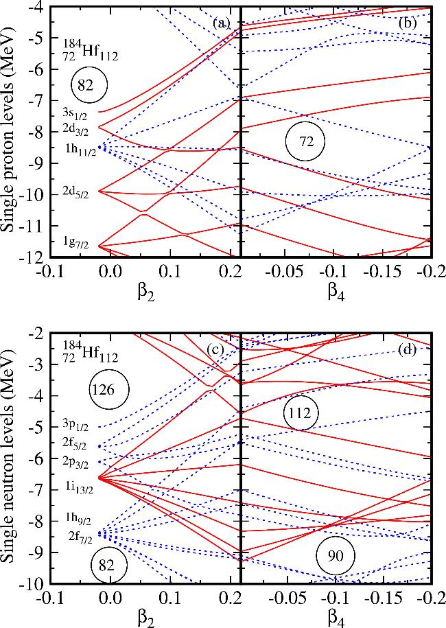
Figure 5. Calculated proton (a, b) and neutron (c, d) single-particle energies as functions of the quadrupole deformation β2 (a, c) and hexadecapole deformation β4 (b, d) for the central nucleus ${}_{72}^{184}$Hf112, focusing on the window of interest near the Fermi surface. Red solid (blue dotted) lines refer to positive and negative parity. In (a) and (c), the single-particle orbitals at β2 = 0.0 are labeled by the spherical quantum numbers nlj and the calculations extend to the equilibrium deformation (β2 = 0.237), for further details, e.g. see table 2. In (b) and (d), the deformation β2 is always set to the equilibrium value. |
Table 2. The calculated single-particle levels near the Fermi surface at β2 = 0.237,γ = 0o and β4 = 0.00 for protons and neutrons in the selected nucleus ${}_{72}^{184}$Hf112,together with their wave-function components expanded in the cylindrical basis ∣NnzΩ⟩ and spherical basis ∣NljΩ⟩.The calculations are performed using the WS Hamiltonian with the cranking parameters.The proton and neutron Fermi levels correspond to the energies −7.95 MeV and −5.43 MeV, respectively. |
| ϵ(MeV) | The first six main-components in terms of ∣NnzΛΩ⟩ (upper) and ∣NljΩ⟩ (lower) | |
|---|---|---|
| Proton | −8.58 | $87.6 \% | 523\frac{7}{2}\rangle +7.7 \% | 514\frac{7}{2}\rangle +2.5 \% | 503\frac{7}{2}\rangle +0.6 \% | 743\frac{7}{2}\rangle +0.5 \% | 303\frac{7}{2}\rangle +0.3 \% | 943\frac{7}{2}\rangle $ |
| 88.4% $| 5{h}_{\frac{11}{2}}\frac{7}{2}\rangle +3.1 \% | 7{j}_{\frac{15}{2}}\frac{7}{2}\rangle +2.7 \% | 5{f}_{\frac{7}{2}}\frac{7}{2}\rangle +1.9 \% | 5{h}_{\frac{9}{2}}\frac{7}{2}\rangle +0.6 \% | 3{f}_{\frac{7}{2}}\frac{7}{2}\rangle +0.6 \% | 9{h}_{\frac{11}{2}}\frac{7}{2}\rangle $ | ||
| −8.49 | $76.3 \% | 411\frac{1}{2}\rangle +6.4 \% | 420\frac{1}{2}\rangle +6.0 \% | 431\frac{1}{2}\rangle +5.0 \% | 211\frac{1}{2}\rangle +1.5 \% | 631\frac{1}{2}\rangle +1.3 \% | 440\frac{1}{2}\rangle $ | |
| 45.1%$| 4{d}_{\frac{3}{2}}\frac{1}{2}\rangle +20.4 \% | 4{d}_{\frac{5}{2}}\frac{1}{2}\rangle +15.0 \% | 4{g}_{\frac{7}{2}}\frac{1}{2}\rangle +3.0 \% | 4{s}_{\frac{1}{2}}\frac{1}{2}\rangle +2.4 \% | 4{g}_{\frac{9}{2}}\frac{1}{2}\rangle +1.9 \% | 2{d}_{\frac{3}{2}}\frac{1}{2}\rangle $ | ||
| −7.95 | $96.1 \% | 404\frac{7}{2}\rangle +3.2 \% | 413\frac{7}{2}\rangle +0.3 \% | 804\frac{7}{2}\rangle +0.2 \% | 624\frac{7}{2}\rangle +0.0 \% | 824\frac{7}{2}\rangle +0.0 \% | 613\frac{7}{2}\rangle $ | |
| 95.0%$| 4{g}_{\frac{7}{2}}\frac{7}{2}\rangle +2.5 \% | 4{g}_{\frac{9}{2}}\frac{7}{2}\rangle +1.3 \% | 6{i}_{\frac{11}{2}}\frac{7}{2}\rangle +0.5 \% | 6{g}_{\frac{7}{2}}\frac{7}{2}\rangle +0.2 \% | 10{g}_{\frac{7}{2}}\frac{7}{2}\rangle +0.2 \% | 8{g}_{\frac{7}{2}}\frac{7}{2}\rangle $ | ||
| −6.94 | 87.9%$| 402\frac{5}{2}\rangle +6.2 \% | 202\frac{5}{2}\rangle +1.7 \% | 602\frac{5}{2}\rangle +1.5 \% | 422\frac{5}{2}\rangle +1.0 \% | 622\frac{5}{2}\rangle +0.7 \% | 802\frac{5}{2}\rangle $ | |
| 86.0%$| 4{d}_{\frac{5}{2}}\frac{5}{2}\rangle +21.2 \% | 2{d}_{\frac{5}{2}}\frac{5}{2}\rangle +15.9 \% | 4{g}_{\frac{7}{2}}\frac{5}{2}\rangle +5.3 \% | 4{g}_{\frac{9}{2}}\frac{5}{2}\rangle +3.4 \% | 6{d}_{\frac{5}{2}}\frac{5}{2}\rangle +2.0 \% | 8{d}_{\frac{5}{2}}\frac{5}{2}\rangle $ | ||
| −6.85 | 95.7%$| 514\frac{9}{2}\rangle +3.0 \% | 505\frac{9}{2}\rangle +0.4 \% | 914\frac{9}{2}\rangle +0.4 \% | 734\frac{9}{2}\rangle +0.4 \% | 934\frac{9}{2}\rangle +0.0 \% | 954\frac{9}{2}\rangle $ | |
| 94.3%$| 5{h}_{\frac{11}{2}}\frac{9}{2}\rangle +2.7 \% | 7{j}_{\frac{15}{2}}\frac{9}{2}\rangle +1.6 \% | 5{h}_{\frac{9}{2}}\frac{9}{2}\rangle +0.8 \% | 9{h}_{\frac{11}{2}}\frac{9}{2}\rangle +0.2 \% | 7{j}_{\frac{13}{2}}\frac{9}{2}\rangle +0.2 \% | 11{h}_{\frac{11}{2}}\frac{9}{2}\rangle $ | ||
| | ||
| Neutron | −6.19 | $86.5 \% | 624\frac{9}{2}\rangle +7.1 \% | 615\frac{9}{2}\rangle +2.1 \% | 604\frac{9}{2}\rangle +1.8 \% | 824\frac{9}{2}\rangle +1.7 \% | 844\frac{9}{2}\rangle +0.4 \% | 404\frac{9}{2}\rangle $ |
| 88.3%$| 6{i}_{\frac{13}{2}}\frac{9}{2}\rangle +3.2 \% | 8{i}_{\frac{13}{2}}\frac{9}{2}\rangle +2.6 \% | 8{k}_{\frac{17}{2}}\frac{9}{2}\rangle +2.0 \% | 6{g}_{\frac{9}{2}}\frac{9}{2}\rangle +1.5 \% | 4{g}_{\frac{9}{2}}\frac{9}{2}\rangle +1.2 \% | 6{i}_{\frac{11}{2}}\frac{9}{2}\rangle $ | ||
| −5.51 | $65.3 \% | 510\frac{1}{2}\rangle +10.4 \% | 521\frac{1}{2}\rangle +6.2 \% | 310\frac{1}{2}\rangle +5.3 \% | 710\frac{1}{2}\rangle +3.5 \% | 730\frac{1}{2}\rangle +2.0 \% | 530\frac{1}{2}\rangle $ | |
| 29.7%$| 5{p}_{\frac{3}{2}}\frac{1}{2}\rangle +25.5 \% | 5{f}_{\frac{5}{2}}\frac{1}{2}\rangle +14.9 \% | 5{f}_{\frac{7}{2}}\frac{1}{2}\rangle +10.0 \% | 5{h}_{\frac{9}{2}}\frac{1}{2}\rangle +6.6 \% | 7{p}_{\frac{3}{2}}\frac{1}{2}\rangle +3.5 \% | 3{p}_{\frac{3}{2}}\frac{1}{2}\rangle $ | ||
| −5.43 | $78.1 \% | 503\frac{7}{2}\rangle +7.8 \% | 703\frac{7}{2}\rangle +7.3 \% | 303\frac{7}{2}\rangle +4.7 \% | 514\frac{7}{2}\rangle +1.5 \% | 723\frac{7}{2}\rangle +0.3 \% | 523\frac{7}{2}\rangle $ | |
| 76.8%$| 5{f}_{\frac{7}{2}}\frac{7}{2}\rangle +9.8 \% | 5{h}_{\frac{9}{2}}\frac{7}{2}\rangle +5.9 \% | 7{f}_{\frac{7}{2}}\frac{7}{2}\rangle +4.0 \% | 3{f}_{\frac{7}{2}}\frac{7}{2}\rangle +2.1 \% | 5{h}_{\frac{11}{2}}\frac{7}{2}\rangle +0.5 \% | 11{f}_{\frac{7}{2}}\frac{7}{2}\rangle $ | ||
| −5.22 | 70.1%$| 512\frac{3}{2}\rangle +9.0 \% | 512\frac{3}{2}\rangle +4.1 \% | 521\frac{3}{2}\rangle +3.3 \% | 712\frac{3}{2}\rangle +2.8 \% | 501\frac{3}{2}\rangle +2.5 \% | 532\frac{3}{2}\rangle $ | |
| 48.2%$| 5{f}_{\frac{5}{2}}\frac{3}{2}\rangle +13.4 \% | 5{h}_{\frac{9}{2}}\frac{3}{2}\rangle +11.6 \% | 5{f}_{\frac{7}{2}}\frac{3}{2}\rangle +11.2 \% | 5{p}_{\frac{3}{2}}\frac{3}{2}\rangle +5.1 \% | 7{f}_{\frac{5}{2}}\frac{3}{2}\rangle +1.9 \% | 3{p}_{\frac{3}{2}}\frac{3}{2}\rangle $ | ||
| −4.72 | 93.6%$| 615\frac{11}{2}\rangle +2.9 \% | 606\frac{11}{2}\rangle +2.3 \% | 815\frac{11}{2}\rangle +1.0 \% | 835\frac{11}{2}\rangle +0.1 \% | 806\frac{11}{2}\rangle +0.0 \% | 1035\frac{11}{2}\rangle $ | |
| 94.7%$| 6{i}_{\frac{13}{2}}\frac{11}{2}\rangle +1.8 \% | 8{k}_{\frac{17}{2}}\frac{11}{2}\rangle +1.7 \% | 8{i}_{\frac{13}{2}}\frac{11}{2}\rangle +1.0 \% | 6{i}_{\frac{11}{2}}\frac{11}{2}\rangle +0.3 \% | 8{k}_{\frac{15}{2}}\frac{11}{2}\rangle +0.2 \% | 12{i}_{\frac{13}{2}}\frac{11}{2}\rangle $ | ||
Table 3. The same as table 2,but β4 = −0.087 and the proton and neutron Fermi levels correspond to the energies −7.62 MeV and −5.91 MeV, respectively. |
| ϵ(MeV) | The first six main-components in terms of NnzΛΩ⟩ (upper) and ∣NljΩ⟩ (lower) | |
|---|---|---|
| Proton | −9.35 | $72.4 \% | 411\frac{1}{2}\rangle +7.7 \% | 420\frac{1}{2}\rangle +5.3 \% | 211\frac{1}{2}\rangle +3.8 \% | 631\frac{1}{2}\rangle +3.8 \% | 431\frac{1}{2}\rangle +3.0 \% | 440\frac{1}{2}\rangle $ |
| 44.9%$| 4{d}_{\frac{3}{2}}\frac{1}{2}\rangle +15.6 \% | 4{g}_{\frac{7}{2}}\frac{1}{2}\rangle +15.4 \% | 4{d}_{\frac{5}{2}}\frac{1}{2}\rangle +7.1 \% | 4{s}_{\frac{1}{2}}\frac{1}{2}\rangle +3.3 \% | 4{g}_{\frac{9}{2}}\frac{1}{2}\rangle +2.7 \% | 2{d}_{\frac{3}{2}}\frac{1}{2}\rangle $ | ||
| −9.27 | 85.8%$| 523\frac{7}{2}\rangle +7.8 \% | 514\frac{7}{2}\rangle +2.6 \% | 303\frac{7}{2}\rangle +1.3 \% | 743\frac{7}{2}\rangle +1.0 \% | 503\frac{7}{2}\rangle +0.5 \% | 963\frac{7}{2}\rangle $ | |
| 82.9%$| 5{h}_{\frac{11}{2}}\frac{7}{2}\rangle +4.7 \% | 5{f}_{\frac{7}{2}}\frac{7}{2}\rangle +4.5 \% | 3{f}_{\frac{7}{2}}\frac{7}{2}\rangle +3.6 \% | 7{j}_{\frac{15}{2}}\frac{7}{2}\rangle +1.5 \% | 5{h}_{\frac{9}{2}}\frac{7}{2}\rangle +1.2 \% | 7{h}_{\frac{11}{2}}\frac{7}{2}\rangle $ | ||
| −7.62 | 95.8%$| 514\frac{9}{2}\rangle +1.8 \% | 734\frac{9}{2}\rangle +1.5 \% | 505\frac{9}{2}\rangle +0.5 \% | 914\frac{9}{2}\rangle +0.2 \% | 954\frac{9}{2}\rangle +0.1 \% | 934\frac{9}{2}\rangle $ | |
| 91.2%$| 5{h}_{\frac{11}{2}}\frac{9}{2}\rangle +4.0 \% | 7{j}_{\frac{15}{2}}\frac{9}{2}\rangle +3.0 \% | 5{h}_{\frac{9}{2}}\frac{9}{2}\rangle +0.7 \% | 7{j}_{\frac{13}{2}}\frac{9}{2}\rangle +0.5 \% | 9{h}_{\frac{11}{2}}\frac{9}{2}\rangle +0.2 \% | 7{h}_{\frac{11}{2}}\frac{9}{2}\rangle $ | ||
| −7.39 | 94.5% $| 404\frac{7}{2}\rangle +2.6 \% | 624\frac{7}{2}\rangle +1.9 \% | 413\frac{7}{2}\rangle +0.3 \% | 633\frac{7}{2}\rangle +0.3 \% | 804\frac{7}{2}\rangle +0.2 \% | 604\frac{7}{2}\rangle $ | |
| $90.0 \% | 4{g}_{\frac{7}{2}}\frac{7}{2}\rangle +3.7 \% | 6{i}_{\frac{11}{2}}\frac{7}{2}\rangle +3.4 \% | 4{g}_{\frac{9}{2}}\frac{7}{2}\rangle +1.9 \% | 6{i}_{\frac{13}{2}}\frac{7}{2}\rangle +0.6 \% | 6{g}_{\frac{7}{2}}\frac{7}{2}\rangle +0.2 \% | 10{g}_{\frac{7}{2}}\frac{7}{2}\rangle $ | ||
| −6.56 | 87.3% $| 402\frac{5}{2}\rangle +4.9 \% | 202\frac{5}{2}\rangle +4.6 \% | 622\frac{5}{2}\rangle +0.9 \% | 413\frac{5}{2}\rangle +0.8 \% | 602\frac{5}{2}\rangle +0.7 \% | 802\frac{5}{2}\rangle $ | |
| $79.5 \% | 4{d}_{\frac{5}{2}}\frac{5}{2}\rangle +5.0 \% | 4{g}_{\frac{7}{2}}\frac{5}{2}\rangle +4.7 \% | 4{g}_{\frac{9}{2}}\frac{5}{2}\rangle +3.8 \% | 6{i}_{\frac{13}{2}}\frac{5}{2}\rangle +2.8 \% | 2{d}_{\frac{5}{2}}\frac{5}{2}\rangle +1.0 \% | 6{i}_{\frac{11}{2}}\frac{5}{2}\rangle $ | ||
| | ||
| Neutron | −6.88 | $84.6 \% | 624\frac{9}{2}\rangle +6.6 \% | 615\frac{9}{2}\rangle +3.2 \% | 844\frac{9}{2}\rangle +2.2 \% | 824\frac{9}{2}\rangle +2.2 \% | 404\frac{9}{2}\rangle +0.9 \% | 604\frac{9}{2}\rangle $ |
| 82.0%$| 6{i}_{\frac{13}{2}}\frac{9}{2}\rangle +4.4 \% | 8{i}_{\frac{13}{2}}\frac{9}{2}\rangle +3.9 \% | 4{g}_{\frac{9}{2}}\frac{9}{2}\rangle +3.5 \% | 6{g}_{\frac{9}{2}}\frac{9}{2}\rangle +3.5 \% | 8{k}_{\frac{17}{2}}\frac{9}{2}\rangle +1.2 \% | 6{i}_{\frac{11}{2}}\frac{9}{2}\rangle $ | ||
| −6.14 | $65.2 \% | 510\frac{1}{2}\rangle +10.7 \% | 521\frac{1}{2}\rangle +6.1 \% | 310\frac{1}{2}\rangle +5.9 \% | 730\frac{1}{2}\rangle +4.9 \% | 710\frac{1}{2}\rangle +1.5 \% | 301\frac{1}{2}\rangle $ | |
| 27.1%$| 5{f}_{\frac{5}{2}}\frac{1}{2}\rangle +23.6 \% | 5{p}_{\frac{3}{2}}\frac{1}{2}\rangle +13.7 \% | 5{f}_{\frac{7}{2}}\frac{1}{2}\rangle +12.5 \% | 5{h}_{\frac{9}{2}}\frac{1}{2}\rangle +5.7 \% | 7{p}_{\frac{3}{2}}\frac{1}{2}\rangle +3.5 \% | 3{p}_{\frac{3}{2}}\frac{1}{2}\rangle $ | ||
| −5.91 | 71.6%$| 512\frac{3}{2}\rangle +8.4 \% | 521\frac{3}{2}\rangle +5.3 \% | 732\frac{3}{2}\rangle +4.3 \% | 312\frac{3}{2}\rangle +3.0 \% | 712\frac{3}{2}\rangle +1.6 \% | 501\frac{3}{2}\rangle $ | |
| 46.9%$| 5{f}_{\frac{5}{2}}\frac{3}{2}\rangle +17.0 \% | 5{h}_{\frac{9}{2}}\frac{3}{2}\rangle +9.0 \% | 5{f}_{\frac{7}{2}}\frac{3}{2}\rangle +8.0 \% | 5{p}_{\frac{3}{2}}\frac{3}{2}\rangle +6.1 \% | 7{f}_{\frac{5}{2}}\frac{3}{2}\rangle +2.2 \% | 3{p}_{\frac{3}{2}}\frac{3}{2}\rangle $ | ||
| −5.27 | 93.2% $| 615\frac{11}{2}\rangle +3.0 \% | 835\frac{11}{2}\rangle +2.1 \% | 815\frac{11}{2}\rangle +1.5 \% | 606\frac{11}{2}\rangle +0.4 \% | 1055\frac{11}{2}\rangle +0.4 \% | 806\frac{11}{2}\rangle $ | |
| $90.7 \% | 6{i}_{\frac{13}{2}}\frac{11}{2}\rangle +3.6 \% | 8{k}_{\frac{17}{2}}\frac{11}{2}\rangle +2.4 \% | 8{i}_{\frac{13}{2}}\frac{11}{2}\rangle +2.1 \% | 6{i}_{\frac{11}{2}}\frac{11}{2}\rangle +0.6 \% | 8{k}_{\frac{15}{2}}\frac{11}{2}\rangle +0.1 \% | 12{i}_{\frac{13}{2}}\frac{11}{2}\rangle $ | ||
| −4.99 | 80.4% $| 503\frac{7}{2}\rangle +6.4 \% | 703\frac{7}{2}\rangle +5.9 \% | 303\frac{7}{2}\rangle +4.2 \% | 723\frac{7}{2}\rangle +2.8 \% | 514\frac{7}{2}\rangle +1.6 \% | 923\frac{7}{2}\rangle $ | |
| $74.9 \% | 5{f}_{\frac{7}{2}}\frac{7}{2}\rangle +7.9 \% | 5{h}_{\frac{9}{2}}\frac{7}{2}\rangle +5.9 \% | 7{f}_{\frac{7}{2}}\frac{7}{2}\rangle +4.1 \% | 5{h}_{\frac{11}{2}}\rangle +3.1 \% | 3{f}_{\frac{7}{2}}\frac{7}{2}\rangle +1.7 \% | 7{j}_{\frac{15}{2}}\frac{7}{2}\rangle $ | ||
According to whether the hexadecapole deformation β4 is included, namely, at two typical deformation points (β2 = 0.237, γ = 0∘, β4 = 0.000) and (β2 = 0.237, γ = 0∘, β4 = −0.087), tables 2 and 3 respectively illustrate the first six wave-function components of proton and neutron single-particle levels near the Fermi surfaces for ${}_{72}^{184}$Hf112. Through influencing the shell gaps and pairing interactions, the single-particle energy levels can determine nuclear internal structure as well as microscopic shell and pairing correction energies [72]. As it is well known, the spherical HO bases ∣NljΩ⟩ and deformed HO bases (cf section 2 ), especially characterized by the asymptotic Nilsson quantum numbers Ω[NnzΛ], are usually used to understand, e.g., multipole interactions related to the deformation mechanism and to block the high-K configurations. In general, the single-particle levels are labeled by the maximum component of these wave functions. In these two tables, we show these two kinds of wave functions. Certainly, the spherical HO wave functions are indirectly obtained from the Moshinsky transformation mentioned above rather than the direct Hamiltonian diagonalization. It might be helpful to point out that the so-called wave-function label will be somewhat meaningless when the mixing of the corresponding wave function is too serious (e.g., the spherical label $| 5{p}_{\frac{3}{2}}\frac{1}{2}\rangle $ for the neutron −5.51-MeV level in table 2). Due to the axial symmetry (triaxial γ deformation is zero), the quantum number Ω (the angular momentum projection on the symmetry axis) is conserved in the two adopted bases. We can see that the largest components of the WS states are more prominent when adopting the deformed-basis expansion than that using the spherical ones since the similarity between the deformed HO and WS potentials is larger. Moreover, the high-j high-Ω single-particle state is relatively pure due to the difficulties of the mixings for such high-Ω states with large energy difference. We note that, similarly to the case of the octupole deformation which leads to the mixing of the states with Δl = Δj = 3, the hexadecapole deformation is expected to mix the states with Δl = Δj = 4. Indeed, it seems that such phenomena occur though we cannot exclude the quadrupole-quadrupole coupling. For instance, as seen in a comparison of the wave-function components of the proton single-particle states, we can observe that the coexisting partners $4.7 \% | 5{f}_{\frac{7}{2}}\frac{7}{2}\rangle \leftrightarrow 3.6 \% | 7{j}_{\frac{15}{2}}\frac{7}{2}\rangle $ in table 3 is more prominent than the partners $3.1 \% | 7{j}_{\frac{15}{2}}\frac{7}{2}\rangle \leftrightarrow 2.7 \% | 5{f}_{\frac{7}{2}}\frac{7}{2}\rangle $ in table 2 for the $| 5{h}_{\frac{11}{2}}\frac{7}{2}\rangle $ state (note that the state is labeled by the largest component) and for the $| 4{d}_{\frac{5}{2}}\frac{5}{2}\rangle $ state, the partner $| 6{i}_{\frac{13}{2}}\frac{5}{2}\rangle $, apparently coexisted for the partners $79.5 \% | 4{d}_{\frac{5}{2}}\frac{5}{2}\rangle \leftrightarrow 3.8 \% | 6{i}_{\frac{13}{2}}\frac{5}{2}\rangle $ at nonzero β4 (see table 3), does not appear in the wave function, at least, in the first six components at β4 = 0.0, indicating the enhanced mixing of the states with Δl = Δj = 4 due to the hexadecapole-hexadecapole interactions.
Based on the MM method of Strutinsky [50], figure 6 exhibits two types of calculated potential-energy curves, focusing on the region around the equilibrium shapes, to denote the effects of β4 on the total potential energy (binding energy) of the selected nuclei 180,182,184Yb, 182,184,186Hf, and 184,186,188W. From this figure, we can evaluate the nuclear stiffness and binding properties near the equilibrium deformations at the selected space (β2, γ, β4). It can be seen that the inclusion of the hexadecapole deformation degree of freedom can enhance the quadrupole deformations of the minima [e.g., the calculated β2 values with and without the consideration of β4 are respectively 0.221 (0.249), which is closer to experimental data 0.234 (0.274), and 0.200 (0.220) for 184W (182Hf)], describing the experimental data better, and lead to the energy reduction (about 1 − 3 MeV) , helping to reproduce the nuclear mass in experiment (see, e.g., [32, 33]). Taking the hexadecapole deformation into account, we here note that all the nuclei will become stiffer near their equilibrium shapes. Far from these minima, one can see from figure 6 that the green and blue curves overlap, indicating that the influence of the hexadecapole deformation β4 cannot be neglected at that moment.
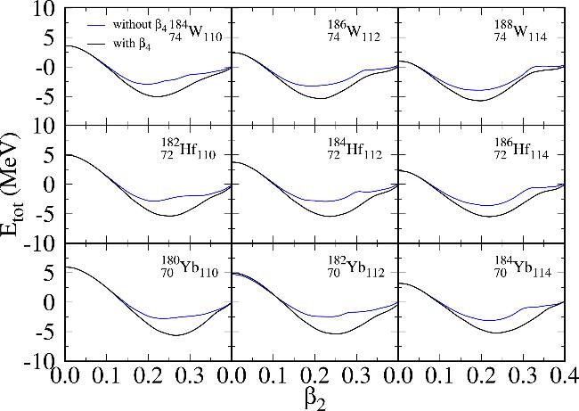
Figure 6. Calculated total energy curves as function of the quadrupole deformation β2 for nine selected even–even nuclei 180−184Yb, 182−186Hf and 184−188W. Note that, at each deformation point β2, the energy is minimized over the triaxial deformation γ and the hexadecapole deformation β4 if β4 is included (e.g., the green line). For more details, see the text. |
The impact of different deformations on the nuclear MoIs is one of our primary concerns in the present project (concerning the pairing effect on the MoIs and the comparison with data, one can refer to [39, 66]). To date, it is known that a large number of ground-state nuclear electric quadrupole moments had been measured in atomic nuclei [73]. These nuclei are deformed and display a low-energy rotational level structure. The corresponding cranking approximations are adopted to explain the rotational spectra, generally by a comparison between theoretical and experimental MoIs. Before starting the microscopic discussion, let us calculate the MOI for a rigid body having the same volume, shape, and density of the nucleus. We know that it has been usual to consider the axially symmetric or asymmetric equilibrium shape [43]. Presently, we perform a generalized treatment for a rigid body which can, in principle, involve any deformation degrees of freedom. As seen in figure 7, the calculated rigid-body MoIs in functions of different deformation parameters are illustrated for the central nucleus 184Hf. It is expected that the microscopic HFBC calculations will give the similar trends, even if considering the pairing effects. From figure 7, one can see that the MoI will rapidly increase (decrease) with increasing quadrupole α20 (α22) deformation parameter. Near the spherical shape, the hexadecapole deformations have a relatively small impact on the MoIs. At the large α4μ (e.g., see α4μ = ±0.3), α42 has the largest influence on the nuclear MoI and the deformation parameters α44 (α40) respectively leads the smallest change in the MoI at positive and negative 0.3 positions. Nevertheless, at the elongated shape, e.g., cf figure 7(b), the effects of different α4μ parameters on MoI obviously increase. From −0.1 to + 0.1, the MoI will increase (decrease) with the increasing α40 (α42). For convenience, let us introduce the sensitivity coefficient of MoI to deformation αλμ, e.g., defined by Sλμ ≡ ∣∂J(1)/∂αλμ∣, to measure to what extent the αλμ deformation will affect the MoI (e.g., in figure 7(a), the sensitivity coefficients satisfy S42 > S43 > S41 > S40 > S44 at the side of α4μ > 0).
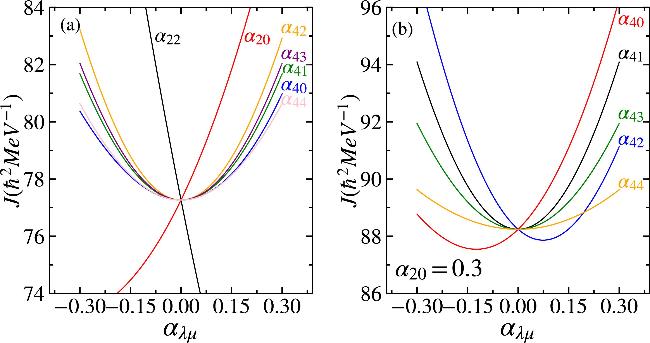
Figure 7. Calculated rigid-body MoIs around the x axis as functions of the deformations α2μ=0,2 and α4μ=0,1,2,3,4 for the central nucleus 184Hf. To see the coupling effect, the deformation α20 is set to 0.3 in (b). Note that the color and order of the labels are in agreement with the curves. |
From figure 7, one can notice that the hexadecapole deformations may have different impacts on the MoIs when the quadrupole deformation is different. To observe the coupling effect, e.g., between α20 and α4μ=0,2,4 degrees of freedom, figure 8 illustrates the calculated rigid-body MoIs in the (α20, α4μ=0,2,4) planes. Relative to the MoI curves in figure 7, one can easily evaluate the MoI at the different combinations of the quadrupole and hexadexapole deformations by such 2D MoI maps. For instance, at α20 ∼ 0.3, a slightly negative α40 or positive α42 deformation will lead to a MoI reduction, agreeing with that in figure 7. Similarly, the MoIs based on the HFBC calculations are also presented in figure 8 (see the corresponding planes on the right-side). Comparing with the contour maps between rigid-body and HFBC calculations, it can indeed be concluded that the MoIs seem to have similar evolution trends no matter whether the pairing effects are included or not. This provides us a way to evaluate the effect of e.g., the exotic deformation degrees of freedom on the nuclear MoI before performing the corresponding microscopic calculations which may be relatively difficult.
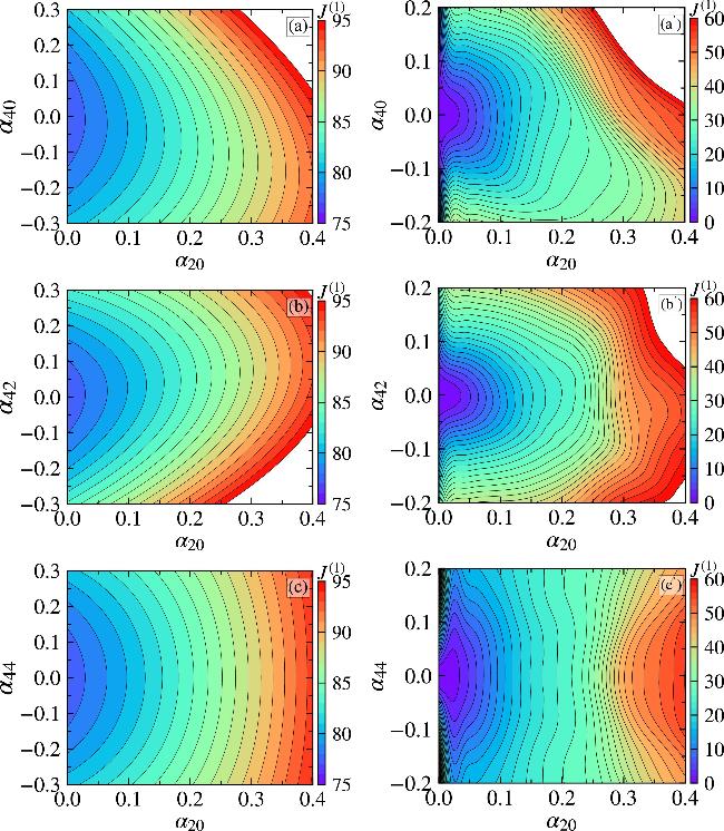
Figure 8. Projections of calculated MoIs on the (β2, α40) (top), (β2, α42) (middle) and (β2, α44) (bottom) planes for the nucleus 184Hf. The maps in the left (a, b, c) and right (a$^{\prime} $, b$^{\prime} $, c$^{\prime} $) sides are respectively obtained by the rigid-body and HFBC calculations (at rotational frequency ℏω = 0.1 MeV). See text for more details. |
For a nuclear state, the excitation energy and angular momentum are usually the observable attributes. In particular, the rotational bands can help to extract the MoI information in experiment. To investigate the rotational damping in the selected 180−184Yb, 182−186Hf and 184−188W nuclei, as seen in figure 9, we illustrate the calculated kinematic MoIs (by the HFBC method mentioned above) of the yrast bands in functions of rotational frequency, along with the experimental data for comparison. During the calculation process, we fixed the shapes of the ground-state values at two cases (with or without the inclusion of β4, cf e.g., table 1), ignoring the shape evolution. Such an approximation seems to be reasonable in these selected nuclei. One can see that the inclusion of the hexadecapole deformation β4 does not affect most of the low-spin and low-lying states qualitatively, but can significantly improve the description of high-spin states of the ground-state bands. For instance, though the data is somewhat scarce, it can still be clearly noticed that the calculated MoIs reproduce the experimental trends, typically, in 182Hf and 186W. In other nuclei, there is no data or too few data points to observe this effect at present. The MoI decrease owing to the negative β4 is in good agreement with our associated discussion of figures 7 and 8. In addition, the current conclusion also agrees with that recently obtained in [16]. The comparison of the MoIs with more data can refer to our previous work, e.g., see [39, 66, 74–77].
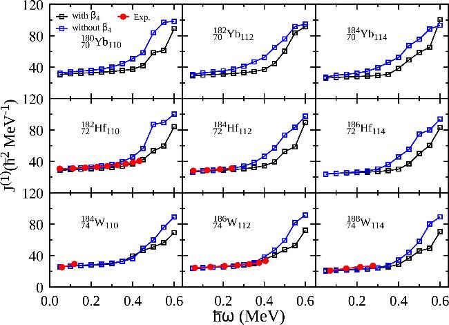
Figure 9. Calculated MoIs, with (black square) and without (blue square) the inclusion of β4 deformations, as functions of rotational frequency for nine selected even–even nuclei 180−184Yb, 182−186Hf and 184−188W, along with the experimental data (red circle). The experimental data are taken from [71]. See text for more explanations. |
From figure 10, it is found that the MoI undergoes a sudden increase during the process of the rotational frequency increase. Such a rapid change in MoI is generally caused by rotation alignments of a pair of nucleons (particularly those occupying high-j low-Ω orbitals near the Fermi surface and usually accompanying shape transition, especially in the soft nucleus). To understand the mechanism of backbending or upbending, we show the aligned angular momenta by the HFBC calculations with fixed ground-state deformations in figure 10, including the proton and neutron contributions, for the selected nine nuclei. One can see that neutrons not only provide more angular alignments but also will be responsible for the MoI anomalies, which indicate that the rapid increase in the MoI is caused by neutron alignment, at least, at ℏω ≤ 0.5 MeV. When ℏω > 0.5 MeV, it seems that the second pair of nucleons (a pair of protons) begins to be broken and aligns along the rotational axis.
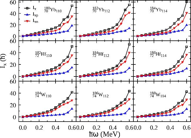
Figure 10. Calculated aligned angular momenta Ix as functions of rotational frequency ℏω for nine selected even–even nuclei 180−184Yb, 182−186Hf and 184−188W, together with the proton Ixp and neutron Ixn components. |
How does the nuclear MoI vary with different deformation (rotational frequency) for fixed frequency ω (shape)? Taking the central nucleus 184Hf as an example, we intend to perform a detailed investigation and answer this question below. For simplicity and clarity, we merely allow one degree of freedom (deformation or rotational frequency) to change during the calculations. figure 11 presents the kinematic MoIs given by the HFBC calculations in functions of ℏω at different β2 and β4 deformations. In figure 11(a), we show the MoIs J(1)(ω), fixing the β2 at different values and setting other deformations to zero. One can see that, for the ground-state case (e.g., at ℏω < 0.2 MeV) in the example nucleus 184Hf, the MoI will increase as the quadrupole deformation β2 deviates from spherical shape (namely, β2 = 0.0). For a spherical nucleus (a spherical quantum many-body system), as expected, the MoI is zero. The nucleus with the prolate shape has the larger MoI value than that of the oblate one at the same deformation amplitudes (e.g., the same ∣β2∣ values). The rapid increase of the MoI for a β2-fixed shape originates from the band crossing (e.g., see the following discussion). We can notice that the band-crossing frequency is somewhat different when fixing different deformation. Generally speaking, the oblate shape has the relatively smaller band-crossing frequency. Similarly, figure 11(b) shows the MoIs in function of ℏω for the cases at different hexadecapole deformation β4, always keeping the equilibrium β2 deformation 0.237 unchanged. From this subplot, one can see that the negative β4 deformation does not change the MoIs at low rotational frequency (e.g., at ℏω≤0.25 MeV) but decreases the MoIs at high rotational frequency, while the positive hexadecapole deformation always increases the MoIs, agreeing with our above results (e.g., see figures 8).
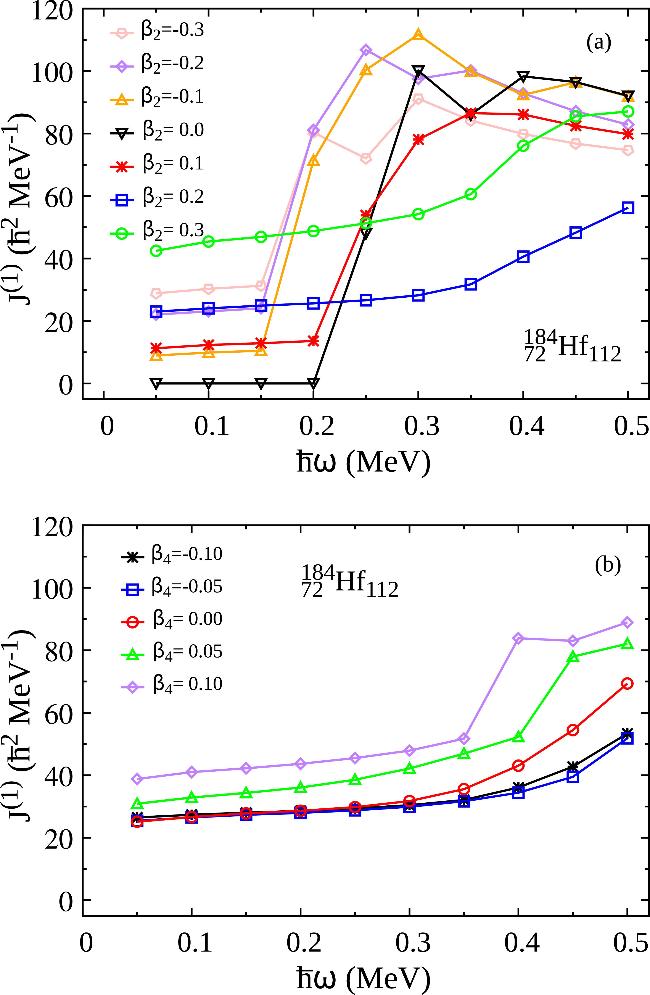
Figure 11. Calculated kinematic MoIs in functions of ℏω at different β2 (a) and β4 (b) deformations for the central nucleus 184Hf. Note that, in subfigure (b), for each β4, the β2 is set to the equilibrium deformation 0.237, e.g., see table 1. |
Similar to figure 11, from the other perspectives, we present the MoI variations at different rotational frequencies in functions of β2 and β4 in figure 12. As can be seen from the figure, at low rotational frequency (e.g. at ℏω = 0.1 MeV), the MoI increases with the increase of ∣β2∣. For the cases of ℏω ≥ 0.2 MeV, at the oblate side, the band crossings will always occur, even, at very weak deformation. At the weak prolate deformation, e.g., β2 = 0.1, the band crossings occur at higher rotational frequencies, e.g., ℏω = 0.3 and 0.4 MeV. The conclusion is that, at low rotational frequency, the increasing ∣β2∣ and positive β4 will lead to the increase of MoI. At the normal deformation case, e.g., β2 ∼ 0.2 − 0.3, the slightly negative β4 will contribute to the decline of the MoIs, at least, in this region. Note that, by the present analysis, we just intend to provide insights into the effect of deformations (especially the hexadecapole one) on the MoI and the practical equilibrium shape should still be determined from the minimum of the potential energy landscape of the nucleon system.
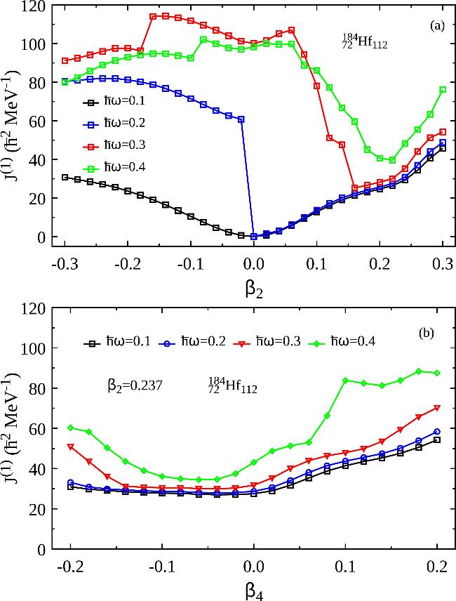
Figure 12. Calculated kinematic MoIs against β2 (a) and β4 (b) at different rotational frequencies ℏω for the central nucleus 184Hf. Similar to figure 11(b), the β2 is fixed to 0.237 in (b). |
To reveal the details of rotation alignments and band crossings to some extent, as seen in figure 13, we show the calculated quasi-particle diagrams for protons and neutrons at three typical deformation points, namely, at β2 = −0.1, 0.1 and 0.2, for the example nucleus 184Hf. The phenomena of low-frequency band crossing appear at, e.g., β2 = −0.1 and 0.1. One can notice that the alignment of proton pair at the positive-parity orbital firstly occurs and then the neutron pair at the negative-parity orbital. Let us remind that the collective angular alignment Ix is the summation of the minus values of the slopes of quasi-particle orbitals [63]. All the quasi-particle orbitals contribute to the collective angular alignment which will change smoothly. However, once the band crossing occurs, the angular alignment will have a rapid increase and, consequently, the MoI will follow the change.
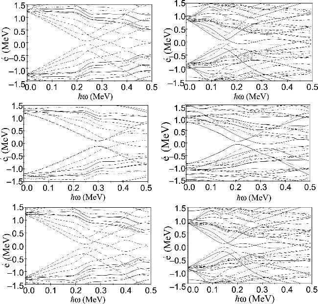
Figure 13. Proton (left) and neutron (right) quasi-particle diagrams at three typical deformation points, namely, β2 = −0.1 (top), +0.1 (middle) and 0.2 (botton), for 184Hf. Note that the oblate deformation β2 = −0.1 is equivalent to the deformation point (β2 = +0.1, γ = −60∘) in the deformation space (β2, γ). |
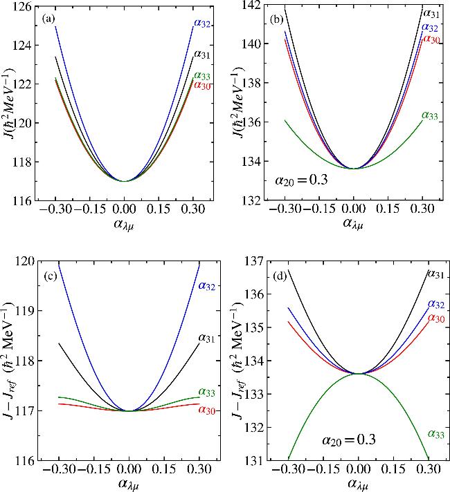
Very recently, the STAR Collaboration provided the first experimental evidence from the high-energy regime for octupole deformation of 238U [78]. Dedes et al [41] discussed the unprecedented experimental identification and properties of the molecular H2O C2v-symmetry rotational band in 236U involved the exotic α3μ=0,1,2,3 deformations. Similar to the cases of the hexadecapole deformations, naturally, it is of interest to understand how these deformations α3μ=0,1,2,3 theoretically affect the MoI in the nucleus. The computing time was qualitatively estimated in typical potential energy calculations, e.g., see [41]. It was illustrated that the high-dimensional potential-energy-surface calculations, due to the huge consumption of CPU time, are still difficult for general computing conditions so far. Before extending the deformation space to include these deformation parameters, it may be meaningful and possible to give a qualitative prediction (even if not quite correctly) based on the rigid-body approximation by considering the corresponding degree(s) of freedom. In figure 14, we firstly present the geometry shapes with different α3μ deformations at an arbitrary deformation amplitude α3μ = 0.3. Similar to figure 7, the rigid-body MoIs around the x axis are illustrated in functions of α3μ=0,1,2,3 in figure 15. Note that, for clarity, only one deformation α3μ is remained to vary, setting others to zero, e.g., cf figure 15(a). To display the quadrupole-octupole coupling, in figure 15(b), the quadrupole deformation α20 is set to 0.3 during the MoI calculation. Indeed, one can find that the sensitivity coefficients Sλμ of MoI to deformation αλμ as defined above (namely, the slope of MoI along the corresponding deformation), are rather different in figures 15 (a) and (b), indicating the coupling effect between quadrupole and octupole deformations. We can see, e.g., at αλμ > 0, that the sensitivity coefficients respectively satisfy S32 > S31 > S33 > S30 and S31 > S32 > S30 > S33 in figures 15(a) and (b). That is to say, in the present case, the α32 and α30 deformations will respectively have the largest and the smallest influences on the nuclear MoI near the spherical shape. Correspondingly, the largest and the smallest influences will respectively come from the deformations α31 and α33 at the elongated shape, and, simultaneously, the sensitivity coefficient S33 significantly reduces. To see more clearly, the calculated rigid-body MoIs after subtracting an arbitrarily selected reference value (e.g., a parabola reference ${J}_{{\rm{ref}}}=56{\alpha }_{\lambda \mu }^{2}$) are illustrated in the subplots (c) and (d) of figure 15. Of course, at this moment, the slope of the curve at αλμ will equal the value of Sλμ − 112αλμ instead of the sensitivity coefficient Sλμ based on the simple mathematical derivation. Further, the microscopic HFBC calculations are of interest and will be done in our future work.
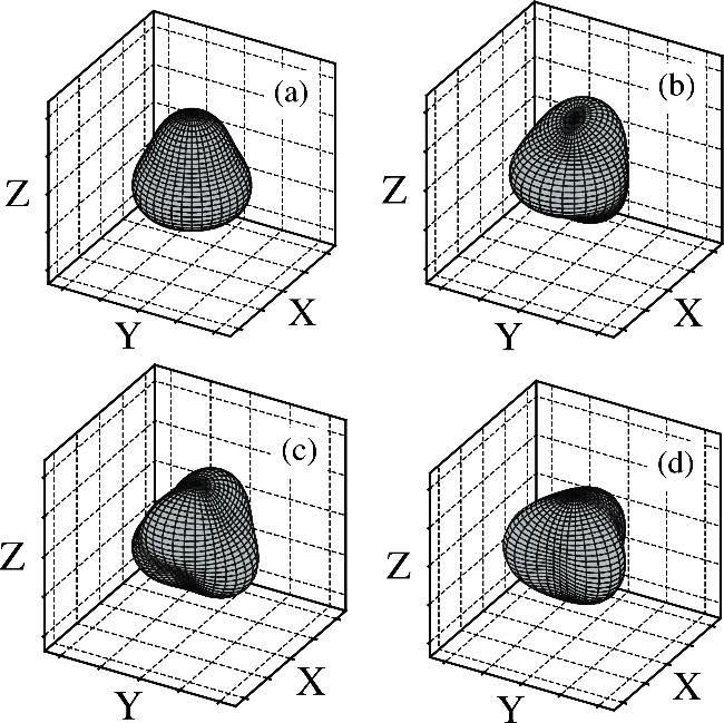
Figure 14. Illustrations of nuclear shapes at single deformation parameter α3μ = +0.3, μ = 0 (a),1 (b), 2 (c), and 3 (d). |
Figure 15. Upper part: Calculated rigid-body MoIs around the x axis in functions of the octupole deformation α3μ=0,1,2,3 for 236U. Bottom part: Similarly, for clarity, the corresponding plots after subtracting a reference value with the MoI ${J}_{{\rm{ref}}}=56{\alpha }_{\lambda \mu }^{2}$ℏ2MeV−1. Note that, in subplots (b) and (d), the quadrupole deformation α20 is set to 0.3 during the MoI calculations with the changing α3μ=0,1,2,3. |
4. Summary and conclusions
In summary, focusing on one of hexadecapole-deformation islands, we have performed an investigation on nuclear ground-state and rotational properties in A ≈ 180 mass region within the theoretical framework of the MM model and cranking shell model. The impact of axial and nonaxial quadrupole and hexadecapole deformation degrees of freedom on nuclear structure (e.g., single-particle levels, equilibrium deformations, MoI, etc.) is analyzed for 184Hf and its eight even–even neighbors 180−184Yb, 182,186Hf and 184−188W. From the present study, the following conclusions may be drawn.
(1) It is found that the inclusion of hexadecapole deformations, especially the axial one α40, can not only enhance nuclear binding and lead to suitable quadrupole deformation β2, but also well reproduce the experimental moments of inertia.
(2) Taking the nucleus 184Hf as an example, we present the evolution properties of MoI with different deformations and rotational frequency by using the HFBC calculation with fixed deformation(s), It is pointed out that understanding the effect of hexadecapole deformation and quadrupole-hexadecapole coupling will be of importance for both nuclear structure and nuclear reaction (e.g., the driving-potential calculation in dinuclear-system model).
(3) Comparing with the calculation of the corresponding deformed rigid body by considering the constant nuclear-density distribution, the present investigation reveals the similarity of the effects of different quadrupole and hexadecapole deformations on nuclear MoI. Combining such a similarity and a recent study, we predict the effects of different exotic deformations have on nuclear rotational properties, e.g., the MoI, and point out the sensitivity of the MoI to different octupole deformation degrees of freedom.
(4) Of course, whether such an exotic deformation will occur depends on the potential-energy-surface calculation rather than that of the MoI. However, this prediction based on the simple rigid-body approximation might still provide us some important information on nuclear level structure once such an exotic deformation occurs.