


1. Introduction
General relativity (GR) foundational theory [1], which describes the geometric characteristics of spacetime, is frequently established. The Friedman equations, which describe the formation of the cosmos, originate from Einstein field equations in an isotropic and homogeneous spacetime. In fact, the framework of GR is a good fit for the big-bang cosmology based on epochs where matter and radiation predominate. The swift expansion of empirical cosmology, which began in the 1990s, demonstrates that the cosmos has gone through two stages of universal acceleration. The first phase is called inflation and the second is the accelerated phase which started after the matter domination. As of now, the cosmos is extending at a quicker rate than already thought, concurring to observational information from type Ia supernova [2], large scale structure and the cosmic microwave background (CMB) [3].
A mysterious component known as dark energy (DE) [4] is believed to drive the current accelerated expansion of the Universe. The cosmological constant is the most fundamental and widely studied candidate for DE, representing a fluid with positive energy density and negative pressure. However, this model faces two major theoretical challenges, the fine-tuning problem and the cosmic coincidence problem [5]. A practical approach to alleviating the coincidence problem involves establishing an interaction between dark matter (DM) and dark energy (DE), as a suitable coupling between them can help explain their comparable energy densities at present.
Despite its significance, the true nature of dark energy remains unknown. To better understand this mysterious component, numerous alternative DE models have been proposed, including the ghost DE model [6], tachyon DE model [7], quintessence, chaplygin gas [8], dilaton, polytropic gas [9], and the holographic dark energy (HDE) model [10].
The gravitational modification of traditional gravity's theory, which results in modified gravities that comprise various constants, depend upon determined properties like torsion, curvature and scalars, etc., is another method for identifying this unusual aspect of the cosmos. A relationship between the ultraviolet and infrared cutoffs was reported by Cohen et al [11], so that a successful field theory can provide a meaningful explanation for nature. A new HDE model is obtained through a change in horizon entropy but it can also be created from changes in area entropy and event horizon. The Sharma-Mittal HDE (SMHDE) model was investigated by Vipin et al [12] and it was shown that the deceleration parameter was linearly connected to the Hubble parameter as q = μ(H) + ν, where μ and ν are constants with arbitrary definitions. After examining several factors, they concluded that the SMHDE model might potentially accelerate the current Universe's expansion.
There are multiple approaches to developed gravitational modification. The simplest is to add new terms in the Einstein–Hilbert Lagrangian which provides new theories such as f(R) theory [13], f(G) theory [14], etc. Another way of modification is to introduce torsion based formulism which results in f(T) gravity [15, 16], f(T, TG) gravity [17], f(T, B) gravity [18], scalar torsion theories [19], etc. Another different class of modifications arises when we introduce equivalent non metricity formulation.
In cosmology, f(Q) theory is a theoretical framework that was created as an alternative to the conventional model, specifically to address several unsolved problems with the understanding of dark energy and the Universe's accelerating expansion. It is a modification of Albert Einstein's GR theory of gravity that uses a function to establish a new type of gravitational interaction. The objectives of f(Q) theory is to introduce a function f(Q), where Q is the non-metricity scalar, into the Einstein–Hilbert action, which regulates GR. The term "non-metricity" describes how the gravitational field modifies the metric of spacetime. Spacetime's deviation from a purely metric-affine geometry is measured by the scalar quantity Q in f(Q) theory.
The formulation of f(Q) theory was mainly determined by the need to offer a framework for understanding the observed acceleration of the Universe's expansion, which is commonly linked to DE. Among the several alternatives to GR and the ΛCDM model, f(Q) theory is still in the early stages of development. It has been investigated in relation to black holes, gravitational wave propagation, and early universe cosmology. At a fundamental stage, the modified f(Q) gravity causes fascinating cosmic phenomena. The standard ΛCDM model may be put to the test f(Q) gravity. 68% of our Universe is DE. Although numerous models have been developed to describe it, nothing is known about it. The holographic principle has been developed for this perspective in modern cosmology in order to address the issue of nature and cosmic expansion. The holographic principle can be written as
$\begin{eqnarray*}\rho =\frac{3{c}^{2}{m}_{{\rm{p}}}^{2}}{{L}^{2}},\end{eqnarray*}$
There have been numerous holographic DE models created with the Sharma-Mittal [20], Renyi [21], and Tsallis [22] models being the most prominent. Sharif and Nazir [23] analyzed the cosmological implications of reconstructed generalized ghost pilgrim DE in f(T, TG) theory. They analyzed the conduct of the equation-of-state (EoS) and deceleration parameters, $\omega -{\omega }^{{\prime} }$ and also r − s planes. They also examine the reconstruction scenario of an anisotropic and spatially homogenous universe model using f(T, TG) gravity [24]. They found that the newly developed HDE f(T, TG) model is consistent within the bounds of b where b is the constant. They showed that there is excellent agreement between all cosmological parameters and observed cosmic behavior [25, 26]. Chattopadhyay et al [27] explored the HDE in f(T) gravity and apply the reconstruction technique to find out the EoS and stability of the model. Waheed [28] applied the reconstruction technique on Tsallis HDE model in extended teleparallel theories of gravity. They found the different cosmological parameters for accelerated expansion of the Universe and also find the stability of the model. Bidlan et al [29] worked on the fractional HDE with scalar and gauge fields and apply the reconstruction technique to find the cosmological parameters.Rao [30] recently worked on SMHDE model in a scalar tensor theory of gravitation. Sharma-Mittal dark energy has been investigated in the framework of Saez-Ballester gravity for Bianchi type-V spacetime by solving the corresponding field equations. The study reveals a transition from decelerated to accelerated cosmic expansion through a dynamic deceleration parameter. Key cosmological diagnostics support the holographic dark energy model and its connection to ΛCDM via statefinder analysis. Saleem et al [31] investigate the cosmic expansion by HDE model in f(Q) gravity. Cosmic evolution has been studied in a gravity theory with a non-metricity scalar using RHDE, SMHDE, and GHDE models in LRS Bianchi type-I spacetime. The models are constructed using a Lambert function-based time-redshift relation with matter as dust and anisotropic fluids. Analysis shows all models are stable and cosmologically viable, with statefinder diagnostics indicating freezing behavior for RHDE and GHDE, and thawing for SMHDE.
Recent developments in holographic dark energy (HDE) models have explored various generalized entropy formalisms, including Barrow and Sharma-Mittal entropies. Barrow entropy introduces a single deformation parameter motivated by quantum gravitational effects and the possible fractal structure of spacetime, leading to modifications in the entropy-area relation. In contrast, Sharma-Mittal entropy offers a two-parameter generalization that unifies Tsallis and Renyi entropies within a non-extensive statistical mechanics framework. This added flexibility enables Sharma-Mittal-based HDE models to capture a broader range of thermodynamic behaviors and cosmological dynamics, including smooth transitions between the quintessence and phantom regimes. While Barrow HDE models [32, 33] have often been explored in the context of extended gravity theories. In the literature, several reconstructions of holographic dark energy have been explored using generalized entropy formalisms, including Rényi, Tsallis, Sharma-Mittal and Barrow entropies. In particular, Barrow entropy–based HDE models have recently been reconstructed in extended gravitational frameworks, such as the studies presented in Eur. Phys. J. C 84 (2024) 1338 and Eur. Phys. J. C 85 (2025) 572. These works modify the holographic bound through a fractal deformation parameter and investigate the resulting cosmological dynamics in modified gravity. Compared to those reconstructions, the present analysis employs the Sharma-Mittal entropy within the f(Q) gravity framework, which offers greater thermodynamic flexibility due to its two-parameter deformation (R, δ). This allows a richer phenomenology and the possibility of unifying several entropy frameworks. Furthermore, by considering three different scale-factor parameterizations (power-law, intermediate and the two unified phases scale factor), our results consistently predict late-time accelerated expansion, providing a broader and more robust reconstruction than previous entropy-based HDE models. Thus, the present study complements and extends earlier works by demonstrating how Sharma-Mittal HDE behaves within symmetric teleparallel gravity and how its predictions compare qualitatively with other entropy-modified reconstructions.
In this work, we consider f(Q) theory with SMHDE model and use different scale factors such as power law, intermediate and unification scale factor. Section 2 offers a concise introduction to f(Q) gravity and presents the reconstruction of the SMHDE model using different scale factor. In Section 3 , we examine these models for each scale factor graphically by using cosmological parameters such as deceleration parameter, EoS parameter, statefinder parameter as well as $\omega -{\omega }^{{\prime} }$ plane. Also, we find the stability of this model for each scale factor. We choose the model of f(Q) = αQn [34], here α should be non-zero and n is the free parameter. The key findings from the preceding sections are summarized in the final section.
2. f(Q) theory
Here, in this section, we discuss the f(Q) theory. We also investigate its field equation. The action of the gravity force f(Q) is described as [35]1 ) in relation to the metric tensor as 1 ) in terms of the relationship leading to 5 ) and equation (4 ) in equation (3 ) we get:
$\begin{eqnarray}\begin{array}{r}S=\displaystyle \int h\left[\frac{1}{2}f(Q)+{{ \mathcal L }}_{{\rm{m}}}\right]{{\rm{d}}}^{4}x.\end{array}\end{eqnarray}$
In the above action, the f(Q) shows the arbitrary non-metricity scalar function Q. The metric determinant is $h=\sqrt{-g}$. The Lagrangian density was ${{ \mathcal L }}_{{\rm{m}}}$. The non-metricity tensor's traces are $\begin{eqnarray*}\begin{array}{r}{Q}_{abc}={{\rm{\nabla }}}_{a}{g}_{bc},\tilde{{Q}_{a}}={Q}_{ab}^{b}.\end{array}\end{eqnarray*}$
Additionally, the super-potential is shown as an expression of tensor of non-metricity as $\begin{eqnarray*}4{P}_{bc}^{a}=-{Q}_{bc}^{a}+2{Q}_{(b\ c)}^{a}-{Q}^{a}{g}_{bc}-\tilde{{Q}_{a}}{g}_{bc}-{\delta }^{a}{\rm{}}_{a}{Q}_{c}.\end{eqnarray*}$
The trace of the above equation is written as $\begin{eqnarray*}Q=-{Q}_{abc}{P}^{abc}.\end{eqnarray*}$
Another important component of this theory is the energy-momentum tensor which can be defined as $\begin{eqnarray}\begin{array}{r}{T}_{bc}=-\frac{2}{\sqrt{-g}}\frac{(\sqrt{-g}{{ \mathcal L }}_{{\rm{m}}})\delta }{\delta {g}^{bc}}.\end{array}\end{eqnarray}$
For the field equations, we require changing in action equation ( $\begin{eqnarray}\begin{array}{rcl}-{T}_{bc} & = & \frac{2}{\sqrt{-g}}{{\rm{\nabla }}}_{a}(\sqrt{-g}{f}_{Q}{P}_{bc}^{a})\\ & & +\frac{1}{2}{g}_{bc}f+{f}_{Q}({P}_{bam}{Q}_{c}^{am}-2{Q}_{amb}{P}_{c}^{am}).\end{array}\end{eqnarray}$
Here, ${f}_{Q}=\frac{\partial f}{\partial Q}$ and f is the general function of non-metricity scalar Q. In addition, we may also consider modification of equation ( $\begin{eqnarray*}\begin{array}{r}{{\rm{\nabla }}}_{b}{{\rm{\nabla }}}_{a}(\sqrt{-g}{f}_{Q}{P}_{bc}^{a})=0.\end{array}\end{eqnarray*}$
The line element of usual Friedmann-Lemaître–Robertson-Walker (FLRW) universe is $\begin{eqnarray}\begin{array}{r}{\rm{d}}{s}^{2}=-{a}^{2}(t){\delta }_{bc}{\rm{d}}{x}^{b}{\rm{d}}{x}^{c}+{\rm{d}}{t}^{2},\end{array}\end{eqnarray}$
here, a(t) is the Universe's scale factor. The preceding line element allows us to express the non-metricity tensor's trace as Q = 6H2. Energy-momentum tensor for perfect fluid can be written as $\begin{eqnarray}\begin{array}{r}{T}_{bc}=(\rho +p){u}_{b}{u}_{c}+p{g}_{bc},\end{array}\end{eqnarray}$
here, p shows the pressure and ρ describes the energy density. Now, with the help of equation ( $\begin{eqnarray}\begin{array}{r}3{H}^{2}={(2{f}_{Q})}^{-1}\left(\frac{f}{2}-\rho \right),\end{array}\end{eqnarray}$
$\begin{eqnarray}\begin{array}{r}3{H}^{2}+\dot{H}+H{\dot{f}}_{Q}{({f}_{Q})}^{-1}={(2{f}_{Q})}^{-1}\left(\frac{f}{2}+p\right).\end{array}\end{eqnarray}$
The f(Q) theory modified Friedmann equations. Here, dot (.) stands for a single time derivative. With the use of the modified Friedmann equations, we may express the Universe's pressure and density as $\begin{eqnarray}\begin{array}{r}\rho =-6{H}^{2}{f}_{Q}+\frac{f}{2},\end{array}\end{eqnarray}$
$\begin{eqnarray}\begin{array}{r}p=-\frac{f}{2}+(3{H}^{2}+\dot{H}+H\frac{{\dot{f}}_{Q}}{{f}_{Q}}),\end{array}\end{eqnarray}$
Also, $\begin{eqnarray*}\begin{array}{rcl}\tilde{\rho } & = & \frac{1}{{f}_{Q}}\left(-\frac{1}{2}f+\rho \right),\\ \tilde{p} & = & H{\dot{f}}_{Q}{({f}_{Q})}^{-1}+\frac{1}{{f}_{Q}}\left(\frac{f}{2}+p\right),\end{array}\end{eqnarray*}$
The dependency on the non-metricity tensor trace will be embedded using the previous equations as elements of a modified tensor of energy-momentum Tbc.Sharma-Mittal investigated the generalized two-parametric entropy which can be expressed as
$\begin{eqnarray}\begin{array}{r}{S}_{{\rm{SM}}}=\frac{1}{R}\left.\left({\left(1+\delta \frac{A}{4}\right)}^{\frac{R}{\delta }}\right)-1\right),\end{array}\end{eqnarray}$
here A = 4πL2, δ and R are the free parameters. Also, Renyi and Tsallis entropies can be retrieved from it by taking into account appropriate bounds of R. When R ⟶ 0 and R ⟶ 1 − δ, respectively, the Sharma-Mittal entropy becomes Renyi entropy and Tsallis entropy. L describes the infrared cut off. The SMHDE model's energy density can be expressed as $\begin{eqnarray*}\begin{array}{r}{\rho }_{D}\propto \frac{{S}_{{\rm{SM}}}}{{L}^{4}},\quad {\rho }_{D}=3{C}^{2}\frac{{S}_{{\rm{SM}}}}{{L}^{4}},\end{array}\end{eqnarray*}$
here C is the constant. In SMHDE model, Hubble radius is taken as infrared cutoff $L=\frac{1}{H}$. The model's energy density can be written as $\begin{eqnarray}\begin{array}{r}\rho =3{C}^{2}{H}^{4}\frac{\left[{\left(\frac{\pi \delta }{{H}^{2}}+1\right)}^{\frac{R}{\delta }}\right]-1}{8\pi R}.\end{array}\end{eqnarray}$
3. Cosmological results of SMHDE f(Q) model
Within this section, we apply reconstructed technique to three different scale factors, i.e., power law scale factor, intermediate scale factor and two unified phases scale factor and obtain the reconstructed function f(Q). By the help of this function, we evaluate EoS parameter ω, deceleration parameter q, $\omega -{\omega }^{{\prime} }$ plane and r − s plane. Also, discuss the stability of this model for different scale factors. We discuss the graphical behaviour of all these cosmological parameters in detail.
3.1. Power-law scale factor
Power law scale factor can be written as 8 ) and (11 ), 12 ), we obtain our reconstructed f(Q) function as
$\begin{eqnarray*}\begin{array}{r}a(t)={a}_{o}{t}^{s},\end{array}\end{eqnarray*}$
The positive values of a0 and s shows the scale factor's current value. By using the above scale factor, the value of Hubble parameter and its time derivative is given as below $\begin{eqnarray}\begin{array}{r}H=\frac{s}{t},\quad \dot{H}=-\frac{s}{{t}^{2}}.\end{array}\end{eqnarray}$
Now, we equate the energy densities to find our reconstructed model. For this purpose, we equate equations ( $\begin{eqnarray}\begin{array}{r}\frac{f}{2}-6{H}^{2}{f}_{Q}=\frac{3{C}^{2}{H}^{4}}{\pi 8R}\left[{\left(\frac{\pi \delta }{{H}^{2}}+1\right)}^{\frac{R}{\delta }}\right]-1\end{array}.\end{eqnarray}$
By solving the above equation and using the equation ( $\begin{eqnarray}\begin{array}{rcl}f(Q) & = & \left(3{c}^{2}{s}^{2}{\left(\frac{{t}^{2}\left(\delta \pi +\frac{{s}^{2}}{{t}^{2}}\right)}{{s}^{2}}\right)}^{R/\delta }-1\right)\\ & & \times {(4\pi R{t}^{2})}^{-1}+{c}_{1}{{\rm{e}}}^{\frac{{t}^{2}}{2{s}^{2}}},\end{array}\end{eqnarray}$
here, c1 is the constant. δ and R are the free parameters. Next, we discuss the graphical behavior of the reconstructed function f(Q) for different values of s such as s1 = 3.3 (red), s2 = 3.4 (green) and s3 = 4 (blue). Also, we introduce the redshift parameter z for the graphical discussion by using $t={\left(\frac{1}{{a}_{0}(z+1)}\right)}^{g}$. Here, a0 = 1 is the present day scale factor and g is the constant exponent. We choose the values of model parameters as: c1 = 0.2, n = 2, δ = 0.5, R = 0.3, g = − 0.8. The reconstructed function f(Q) (figure 1) shows a decreasing behavior with redshift, starting from a high value at z = 0 and gradually decreasing up to z = 1.5. This behavior reflects the expected evolution of dark energy, which becomes dominant only at late times. The smooth decay indicates the model is stable and consistent with observational cosmology, supporting the viability of our model.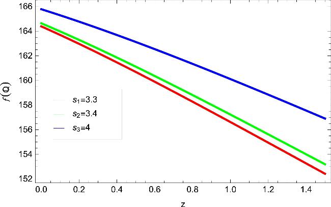
Figure 1. Plot of reconstructed function f(Q) for power law scale factor. |
Next, we discuss the EoS parameter [36] $\omega =\frac{p}{\rho }$ for power law scale factor with SMHDE in f(Q) gravity. By using equations (9 ) and (11 ), we get our EoS parameter for SMHDE model as
$\begin{eqnarray}\begin{array}{rcl}\omega & = & \left(8-\frac{\alpha {\left(\frac{6{s}^{2}}{{t}^{2}}\right)}^{n}}{2}+2\alpha n{\left(\frac{6{s}^{2}}{{t}^{2}}\right)}^{n-1}\right.\\ & & \left.\times \left(-\frac{s}{{t}^{2}}+\frac{3{s}^{2}}{{t}^{2}}+\frac{s(n-1){\left(\frac{6{s}^{2}}{{t}^{2}}\right)}^{n-2}}{t{\left(\frac{6{s}^{2}}{{t}^{2}}\right)}^{n-1}}\right)\right)\\ & & \times {t}^{4}\pi R){\left(3{c}^{2}{s}^{4}\left({\left(\frac{\pi \delta {t}^{2}}{{s}^{2}}+1\right)}^{\frac{R}{\delta }}-1\right)\right)}^{-1}.\end{array}\end{eqnarray}$
The derivative of ω w.r.t t is: $\begin{eqnarray*}\begin{array}{rcl}{\omega }^{{\prime} } & = & -\left(8\pi \alpha {6}^{n}R{t}^{3}{\left(\frac{{s}^{2}}{{t}^{2}}\right)}^{n}{\left(\frac{{s}^{2}+\pi \delta {t}^{2}}{{s}^{2}}\right)}^{R/\delta }\right.\\ & & \times \left({n}^{2}(\pi {t}^{5}\left(R-\frac{9\delta }{2}\right)+18\pi \delta {s}^{3}{t}^{2}\right.\\ & & +{s}^{2}\left(-6\pi \delta {t}^{2}-\frac{9{t}^{3}}{2}\right)+18{s}^{5}-6{s}^{4})\\ & & +{n}^{3}\left({s}^{2}{t}^{3}+\pi \delta {t}^{5}\right)\\ & & +n(18\pi {s}^{3}{t}^{2}\left(R-\frac{5\delta }{2}\right)\\ & & -6{s}^{2}{t}^{2}\left(\pi (R-2\delta )-\frac{7t}{12}\right)-\pi {t}^{5}\left(R-\frac{7\delta }{2}\right)\\ & & \left.-45{s}^{5}+12{s}^{4})-9{s}^{3}\left(\pi {t}^{2}(R-2\delta )-2{s}^{2}\right)\right)\\ & & -\left({n}^{2}\left(18{s}^{3}-6{s}^{2}-\frac{9{t}^{3}}{2}\right)\right.\\ & & \left.+{n}^{3}{t}^{3}+n\left(-45{s}^{3}+12{s}^{2}+\frac{7{t}^{3}}{2}\right)+18{s}^{3}\right)\\ & & \times \left.\left({s}^{2}+\pi \delta {t}^{2}\right)\right)\\ & & \times {\left(27{c}^{2}{s}^{7}\left({s}^{2}+\pi \delta {t}^{2}\right){\left({\left(\frac{{s}^{2}+\pi \delta {t}^{2}}{{s}^{2}}\right)}^{R/\delta }-1\right)}^{2}\right)}^{-1}\end{array}.\end{eqnarray*}$
Figure 2 (left panel) shows the graphical behavior of EoS parameter ω against the redshift parameter z. We use the same values for these graph which we discuss earlier, here α = − 0.2. Figure 2, the reconstructed EoS parameter ω starts near the cosmological constant value of −1 at redshift z ≈ 0.2 and increases rapidly, reaching approximately −0.4. This dark-energy component consistently lies in the quintessence regime throughout the redshift interval considered. The fact that ω approaches −1 at lower redshift suggests that the model behaves similarly to a cosmological constant in the recent Universe, while the gradual increase toward ω = − 0.9 at earlier times indicates a dynamically evolving, non-phantom dark-energy component. This monotonic evolution implies a mild weakening of the negative pressure of dark energy as we move to higher redshift, consistent with a slowly rolling scalar-field-like behavior.
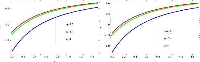
Figure 2. Plot of EoS parameter ω and deceleration parameter q for power law scale factor. |
A useful tool for analyzing the change from deceleration to acceleration is the deceleration parameter q. There are distinct phases for this: q < 0 describes the Universe's acceleration phase, q = 0 shows that the Universe is expanding steadily and q > 0 corresponds to the Universe's deceleration behavior. We can evaluate the deceleration parameter for SMHDE model in f(Q) gravity by using the following expression: 15 ) in equation (16 ), we obtain the deceleration parameter as:
$\begin{eqnarray}\begin{array}{r}q=\frac{1}{2}(3\omega +1),\end{array}\end{eqnarray}$
Using equation ( $\begin{eqnarray*}\begin{array}{rcl}q & = & \left(4\pi {6}^{n}\alpha {t}^{4}R\left(\left(18n-9\right){s}^{3}-6n{s}^{2}\right.\right.\\ & & \left.+n{t}^{3}(n-1)\right){\left(\frac{{s}^{2}}{{t}^{2}}\right)}^{n}\\ & & \left.+9{c}^{2}{s}^{7}\left({\left(\frac{\pi \delta {t}^{2}+{s}^{2}}{{s}^{2}}\right)}^{\frac{R}{\delta }}-1\right)\right)\\ & & \times {\left(18\left({\left(\frac{\pi \delta {t}^{2}+{s}^{2}}{{s}^{2}}\right)}^{\frac{R}{\delta }}-1\right){c}^{2}{s}^{7}\right)}^{-1}.\end{array}\end{eqnarray*}$
Figure 2 (right panel) expresses the graph of deceleration parameter. The deceleration parameter q ≈ −1 when z ≈ 0.2, indicating a phase of exponential expansion at this epoch. The deceleration parameter q is directly influenced by the dark-energy EoS. Since both ω and q exhibit similar increasing trends with redshift, this indicates that the expansion dynamics of the Universe follow the evolution of the dark-energy sector in a consistent manner. he consistency between ω and q further confirms that the model predicts a Universe transitioning from a stronger late-time acceleration toward a milder acceleration at earlier epochs.The $\omega -{\omega }^{{\prime} }$ plane was first developed by Caldwell and Linder [37] who graphically illustrate the various stages of the quintessence DE. The plane $\omega -{\omega }^{{\prime} }$ used to assess how well different DE models perform. The ${\omega }^{{\prime} }$ indicates derivative of ω with respect to t. If ω < 0 as well as ${\omega }^{{\prime} }\lt 0$, it shows the freezing region and in this region, energy density will never be changed. On the other hand, if ω < 0 and ${\omega }^{{\prime} }\gt 0$ show the thawing region in this region, energy density will be increases. The behaviour of $\omega -{\omega }^{{\prime} }$ plane is shown in figure 3. This plot illustrates the thawing region in the $\omega -{\omega }^{{\prime} }$ plane, figure 3 shows that dark energy behaved like a cosmological constant in the past, but is now slowly beginning to evolve as the underlying quintessence field becomes active.
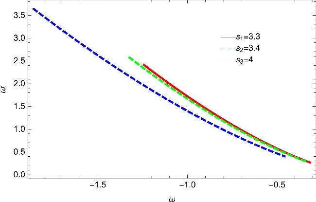
Figure 3. Plot of $\omega -{\omega }^{{\prime} }$ plane for power law scale factor. |
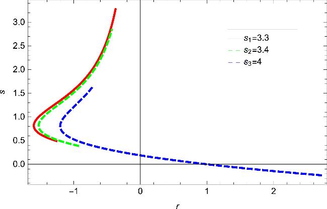
Figure 4. Plot of r − s plane for power law scale factor. |
Sahni et al [38] introduced two dimensionless parameters r and s, known as statefinder parameters, to explain the DE phenomenon. Mathematically, we can write these parameters as follows 18 ) and (23 ), we get the statefinder parameters for our model which are as follows:
$\begin{eqnarray}\begin{array}{r}r=\frac{\dddot{a}}{{H}^{3}a},\quad s={\left(3\left(-\frac{1}{2}+q\right)\right)}^{-1}(r-1).\end{array}\end{eqnarray}$
The jerk parameter r can also be written as $\begin{eqnarray}\begin{array}{r}r=2{q}^{2}+q-\dot{q}.\end{array}\end{eqnarray}$
The Jerk parameter is denoted by r. For flat r = 1, ΛCDM model [39]. The statefinder parameter trajectories in figure 4 demonstrate different cosmic phases such as (s, r) = (1, 1) for CDM model and (s, r) = (1, 0) for ΛCDM model. Also, s > 0 and r < 1 range denotes quintessence and phantom eras of DE were as chaplygin gas model is indicated by the s < 0 with r > 1 range. Now, by using equations ( $\begin{eqnarray*}\begin{array}{rcl}r & = & \left(81{c}^{4}{s}^{14}\left(\pi \delta {t}^{2}+{s}^{2}\right){\left({\left(\frac{\pi \delta {t}^{2}+{s}^{2}}{{s}^{2}}\right)}^{\frac{R}{\delta }}\right)}^{2}\right.\\ & & +36{s}^{7}{c}^{2}\left(\pi \alpha {t}^{3}R\right.\\ & & \times \left(9n\,{t}^{3}\left(\pi \delta {t}^{2}+{s}^{2}\right){6}^{n-1}+(18\left(n+\frac{3t}{2}-2\right)\right.\\ & & \times \left(n-\frac{1}{2}\right){s}^{5}-6\left(n+\frac{3t}{2}-2\right)n{s}^{4}\\ & & +18\pi {t}^{2}\left(\delta n+\frac{3}{2}t\delta +R-2\delta \right)\left(n-\frac{1}{2}\right)\\ & & \times {s}^{3}-6\left(\left(\delta n+\frac{3}{2}t\delta +R-2\delta \right)\pi \right.\\ & & -\left.\frac{\left(\left(\frac{3n}{2}-\frac{3}{2}\right)t+{n}^{2}-\frac{9n}{2}+2\right)t}{6}\right){t}^{2}n\,{s}^{2}\\ & & +\left(\frac{3\delta \left(n-1\right)t}{2}+\left(n-1\right)R\right.\\ & & +\left.\left.\left(n-4\right)\delta \left(n-\frac{1}{2}\right)\right)\pi {t}^{5}n){6}^{n}\right){\left(\frac{{s}^{2}}{{t}^{2}}\right)}^{n}\\ & & -\left.\frac{9{c}^{2}{s}^{7}\left(\pi \delta {t}^{2}+{s}^{2}\right)}{2}\right){\left(\frac{\pi \delta {t}^{2}+{s}^{2}}{{s}^{2}}\right)}^{\frac{R}{\delta }}\\ & & +8\left(\pi \delta {t}^{2}+{s}^{2}\right)\left({\pi }^{2}{\left({6}^{n}\right)}^{2}{\alpha }^{2}{t}^{8}{R}^{2}\left(\left(18n-9\right){s}^{3}\right.\right.\\ & & -{\left.6n\,{s}^{2}+n\,{t}^{3}\left(n-1\right)\right)}^{2}{\left({\left(\frac{{s}^{2}}{{t}^{2}}\right)}^{n}\right)}^{2}\\ & & -\left(81\left({6}^{n-1}n\,{t}^{3}+\left({6}^{n}\left(18\left(n+\frac{3t}{2}-2\right)\right.\right.\right.\right.\\ & & \times \left(n-\frac{1}{2}\right){s}^{3}-6\left(n+\frac{3t}{2}-2\right)n\,{s}^{2}\\ & & \left.\left.+{t}^{3}n\left(\left(\frac{3n}{2}-\frac{3}{2}\right)t+{n}^{2}-\frac{9n}{2}+2\right)\right)\right)\\ & & \times \left.\left.\left.\left.{(9)}^{-1}\right){s}^{7}{c}^{2}\pi \alpha {t}^{3}R{\left(\frac{{s}^{2}}{{t}^{2}}\right)}^{n}\right){(2)}^{-1}+\frac{81{c}^{4}{s}^{14}}{8}\right)\right)\\ & & \times {\left(81{s}^{14}{c}^{4}\left(\pi \delta {t}^{2}+{s}^{2}\right){\left({\left(\frac{\pi \delta {t}^{2}+{s}^{2}}{{s}^{2}}\right)}^{\frac{R}{\delta }}-1\right)}^{2}\right)}^{-1}.\end{array}\end{eqnarray*}$
Since the equation for s is a bit lengthy, we are not including it here. The graph presents a statefinder diagnostic in the (r, s) plane, displaying three trajectories corresponding to different cosmological models. The red and green curves stay close to the quintessence-like region, indicating only small changes in the dark-energy behavior. The blue curve behaves differently–it moves through the ΛCDM point (r = 1, s = 0), briefly matching the standard cosmological model, and then shifts toward a Chaplygin-like regime, showing a much stronger deviation from cosmological-constant behavior.Lastly, we investigate the stability of SMHDE model in f(Q) with the help of squared speed of sound parameter which can be written as 8 ) with equation (12 ) and put the values in equation (19 ), we get our speed square of sound parameter, which is:
$\begin{eqnarray}\begin{array}{r}{v}_{{\rm{s}}}^{2}=\dot{p}/\dot{\rho }\end{array}.\end{eqnarray}$
The positive behavior of this parameter shows the stability of the model whereas the negative behavior shows that the given model is unstable. Now by using equation ( $\begin{eqnarray*}\begin{array}{rcl}{v}_{{\rm{s}}}^{2} & = & -\left(4\left(\pi \delta {t}^{2}+{s}^{2}\right)\pi {\left(\frac{{s}^{2}}{{t}^{2}}\right)}^{n}{6}^{n}\alpha {t}^{4}nR\right.\\ & & \times \left.\left(\left({n}^{2}-\frac{5}{2}n+\frac{3}{2}\right){t}^{3}+\left(18n-9\right){s}^{3}-6n{s}^{2}\right)\right)\\ & & \times \left(27\left(\left(\pi \left(R-2\delta \right){t}^{2}-2{s}^{2}\right)\right.\right.\\ & & \times {\left.\left.{\left(\frac{\pi \delta {t}^{2}+{s}^{2}}{{s}^{2}}\right)}^{\frac{R}{\delta }}+2\pi \delta {t}^{2}+2{s}^{2}\right){s}^{7}{c}^{2}\right)}^{-1}.\end{array}\end{eqnarray*}$
Figure 5 shows the stable behavior for power-law scale factor which means SMHDE model f(Q) gravity stable for all three values of s.
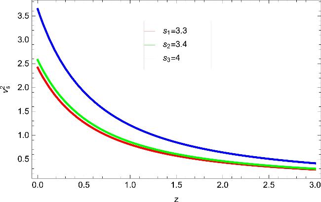
Figure 5. Plot of ${v}_{s}^{2}$ for power law scale factor. |
3.2. Intermediate scale factor
Here, we explore the intermediate scale factor, a distinct expansion law that interpolates between power-law and exponential behaviors. This formulation provides a versatile tool in modeling early universe dynamics, particularly within inflationary frameworks, which has the following expression:
$\begin{eqnarray}\begin{array}{r}a(t)=\exp (a{t}^{{m}}),\end{array}\end{eqnarray}$
here a is an arbitrary constant which controls the expansion rate and 0 < m < 1. Hubble parameter for this scale factor can be express as $\begin{eqnarray}\begin{array}{r}H(t)=a{m}{t}^{{m}-1},\end{array}\end{eqnarray}$
By equating equation (11 ) with equation (8 ) and substituting equation (21 ) into the resulting expression, we obtain the reconstructed function corresponding to this model as 9 ) and (11 ), we obtain EoS parameter ω.
$\begin{eqnarray*}\begin{array}{rcl}f(Q) & = & {{\rm{e}}}^{\frac{{t}^{-2m+2}Q}{12{a}^{2}{m}^{2}}}{c}_{1}+\left(3{a}^{2}{m}^{2}{t}^{2m-2}{c}^{2}\right.\\ & & \times \left.\left({\left(\frac{{a}^{2}{m}^{2}+{t}^{-2m+2}\pi \delta }{{a}^{2}{m}^{2}}\right)}^{\frac{R}{\delta }}-1\right)\right){(4\pi R)}^{-1}.\end{array}\end{eqnarray*}$
Figure 6 shows the reconstructed function for intermediate scale factor of SMHDE model in f(Q) gravity. The graph represents the decreasing behavior of reconstructed function f(Q) for all three values of m = 0.75, 0.79, 0.8 and the values of other parameters are: R = 0.8, δ = 0.5, a = 0.7, c1 = 1.9 and g = 2.4. By using equations ( $\begin{eqnarray*}\begin{array}{rcl}\omega & = & \left(4\left(\left({n}^{2}-n\right){t}^{-7m+7}\right.\right.\\ & & +6{a}^{2}\left(n\left(m-1\right){t}^{-5m+4}\right.\\ & & +3\left.\left.\left(n-\frac{1}{2}\right)a\,{t}^{-4m+4}m\right){m}^{2}\right)\\ & & \left.\times {6}^{n}\pi \alpha {\left({a}^{2}{m}^{2}{t}^{2m-2}\right)}^{n}R\right)\\ & & \times {\left(27\left({\left(\frac{{a}^{2}{m}^{2}+{t}^{-2m+2}\pi \delta }{{a}^{2}{m}^{2}}\right)}^{\frac{R}{\delta }}-1\right){c}^{2}{a}^{7}{m}^{7}\right)}^{-1}\end{array}.\end{eqnarray*}$
and ${\omega }^{{\prime} }$ is written as follows: $\begin{eqnarray}\begin{array}{rcl}{\omega }^{{\prime} } & = & \left(16\,{6}^{n}\left(\left(3\left(n-\frac{1}{2}\right)\pi {a}^{3}\left(\delta n\right.\right.\right.\right.\\ & & \left.+R-2\delta \right){m}^{3}{t}^{5-4m}\\ & & +\left(\pi \left(n-1\right)n\left(\delta n+R-\frac{7}{2}\delta \right){t}^{8-7m}\right){(6)}^{-1}\\ & & +{a}^{2}{m}^{2}\left(\pi (\left(\delta n-\frac{5}{2}\delta +R\right)m\right.\\ & & -\delta n-R+2\delta )n\,{t}^{5-5m}\\ & & +\left(\frac{1}{6}{n}^{3}-\frac{3}{4}{n}^{2}+\frac{7}{12}n\right){t}^{-5\,m+6}\\ & & +{a}^{2}{m}^{2}\left(n\left(\left(n-\frac{5}{2}\right)m-n+2\right){t}^{-3\,m+3}\right.\\ & & +\left.\left.\left.3\left(n-2\right)\left(n-\frac{1}{2}\right)am\,{t}^{-2\,m+3}\right)\right)\right)\\ & & \times {(({a}^{2}{m}^{2}+{t}^{-2\,m+2}\pi \delta ){({a}^{2}{m}^{2})}^{-1})}^{\frac{R}{\delta }}\\ & & -3\left(n-2\right)\left(n-\frac{1}{2}\right)\pi {a}^{3}{m}^{3}\delta {t}^{5-4m}\\ & & -\left(\pi \left(n-1\right)\delta n\left(n-\frac{7}{2}\right){t}^{8-7m}\right){(6)}^{-1}\\ & & -\left(\pi \delta n\left(\left(n-\frac{5}{2}\right)m-n+2\right){t}^{5-5m}\right.\\ & & +\left(\frac{1}{6}{n}^{3}-\frac{3}{4}{n}^{2}+\frac{7}{12}n\right){t}^{-5\,m+6}\\ & & +{a}^{2}{m}^{2}\left(n\left(\left(n-\frac{5}{2}\right)m-n+2\right){t}^{-3\,m+3}\right.\\ & & +3\left.\left.\left.\left(n-2\right)\left(n-\frac{1}{2}\right)am\,{t}^{-2\,m+3}\right)\right){a}^{2}{m}^{2}\right)\\ & & \left.\times \pi {\left({a}^{2}{m}^{2}{t}^{2\,m-2}\right)}^{n}\alpha \left(m-1\right)R\right)\\ & & \times \left(9{c}^{2}{a}^{7}{m}^{7}{\left({\left(\frac{{a}^{2}{m}^{2}+{t}^{-2\,m+2}\pi \delta }{{a}^{2}{m}^{2}}\right)}^{\frac{R}{\delta }}-1\right)}^{2}\right.\\ & & \times {\left.\left({a}^{2}{m}^{2}{t}^{2m}+\pi \delta {t}^{2}\right)\right)}^{-1}.\end{array}\end{eqnarray}$
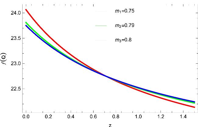
Figure 6. Plot of reconstructed function f(Q) for intermediate scale factor. |
Plot ω graphically in figure 7 against redshift z. The graph of EoS increases with redshift means the Universe had a decelerated phase in the past and transitions to an accelerated phase at late times, with dark energy becoming more negative (phantom-like) as the Universe evolves. Using equation (16 ), we get the deceleration parameter q, which is written as follows:
$\begin{eqnarray*}\begin{array}{rcl}q & = & \left(4\left(\left({n}^{2}-n\right){t}^{-7m+7}\right.\right.\\ & & +6{a}^{2}\left(n\left(m-1\right){t}^{-5m+4}\right.\\ & & +3\left.\left.\left(n-\frac{1}{2}\right)a\,{t}^{-4m+4}m\right){m}^{2}\right)\\ & & \times {6}^{n}\pi \alpha R{\left({a}^{2}{m}^{2}{t}^{2m-2}\right)}^{n}+9{c}^{2}{a}^{7}{m}^{7}\\ & & \times \left.\left({\left(\frac{{a}^{2}{m}^{2}+{t}^{-2m+2}\pi \delta }{{a}^{2}{m}^{2}}\right)}^{\frac{R}{\delta }}-1\right)\right)\\ & & \times {\left(18\left({\left(\frac{{a}^{2}{m}^{2}+{t}^{-2m+2}\pi \delta }{{a}^{2}{m}^{2}}\right)}^{\frac{R}{\delta }}-1\right){c}^{2}{a}^{7}{m}^{7}\right)}^{-1}.\end{array}\end{eqnarray*}$
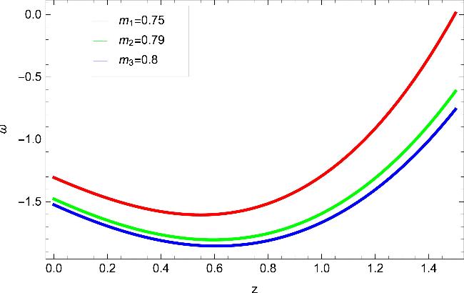
Figure 7. Plot of EoS parameter ω for intermediate scale factor. |
We plot the graph of q by taking the values the same as we discussed earlier, against redshift 0 < z < 1.5. Figure 8 shows the evolution of the deceleration parameter q with redshift. The parameter increases as we look back in time, starting from negative values today (q < 0), indicating accelerated expansion for m = 0.79, 0.8 and for m = 0.75 crossing zero at an intermediate redshift. At higher redshifts q > 0 for the value, the Universe was in a decelerated phase dominated by matter or radiation. This behavior clearly illustrates a transition from deceleration in the past to acceleration in the recent Universe.
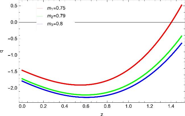
Figure 8. Plot of deceleration parameter q for intermediate scale factor. |
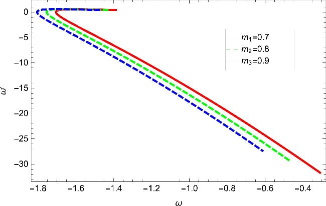
Figure 9. Plot of $\omega -{\omega }^{{\prime} }$ plane for intermediate scale factor. |
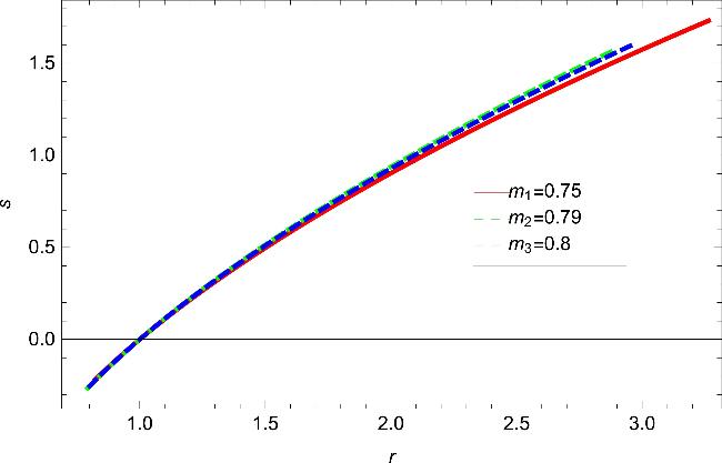
Figure 10. Plot of (r − s) plane for intermediate scale factor. |
Now, by substituting equation (21 ) in equations (23 ) and (18 ), we obtain the expressions for r and s parameters which are too lengthy expressions. So, the jerk and snap parameters are shown in figure 9. The evolution of the statefinder parameters r and s in figure 10 shows that the model starts at the ΛCDM point (r = 1, s = 0), behaving like a cosmological constant. As r and s increase, the Universe departs from ΛCDM, indicating enhanced acceleration and the presence of a dynamical dark energy component. The final values (r = 3, s = 1.5) suggest a significantly stronger acceleration compared to the standard ΛCDM scenario.
Next, we found the squared speed of sound parameter for intermediate scale factor with the help of equation (19 ) and equation (8 ) and use equation (21 ), we get our speed square of sound parameter:
$\begin{eqnarray*}\begin{array}{rcl}{v}_{{\rm{s}}}^{2} & = & -\left(8{\left({a}^{2}{m}^{2}{t}^{2m-2}\right)}^{n}\alpha nR(({6}^{n}\pi \delta \left(n-1\right)\right.\\ & & \times \left(m-1\right){t}^{-7m+9}){(36)}^{-1}\\ & & +{m}^{2}{a}^{2}\left(\frac{{6}^{n}\left(n-1\right)\left(m-1\right){t}^{-5m+7}}{36}\right.\\ & & -\left(\left(-\frac{{6}^{1+n}{m}^{2}}{18}+{6}^{n}\left(m-\frac{2}{3}\right)\right)\right.\\ & & \times \left.\delta \pi {t}^{-5m+6}\right){(2)}^{-1}\\ & & +\left(-\frac{m\left(-\frac{{6}^{1+n}{m}^{2}}{18}+{6}^{n}\left(m-\frac{2}{3}\right)\right)a\,{t}^{-3m+4}}{2}\right.\\ & & \left.+{6}^{n}\left(m-1\right)\left({t}^{4-2m}{a}^{2}{m}^{2}+{t}^{6-4m}\pi \delta \right)\right)\\ & & \left.\left.\times ma\right))\pi \right)\left(3{c}^{2}\left(\left(-2{a}^{2}{m}^{2}{t}^{2m}+{t}^{2}\pi \left(R-2\delta \right)\right)\right.\right.\\ & & \times {\left(\frac{{a}^{2}{m}^{2}+{t}^{-2m+2}\pi \delta }{{a}^{2}{m}^{2}}\right)}^{\frac{R}{\delta }}+2{a}^{2}{m}^{2}{t}^{2m}\\ & & {\left.\left.+2\pi \delta {t}^{2}\right){m}^{7}\left(m-1\right){a}^{7}\right)}^{-1}.\end{array}\end{eqnarray*}$
Figure 11 shows the stability parameter increases with redshift, starting from a negative value today ${v}_{{\rm{s}}}^{2}\lt 0$, indicating that the model is unstable at the present epoch. At higher redshift, the parameter becomes positive ${v}_{{\rm{s}}}^{2}\gt 0$, showing that the system was stable in the early Universe. This suggests that the model evolves from a unstable phase to the stable phase.
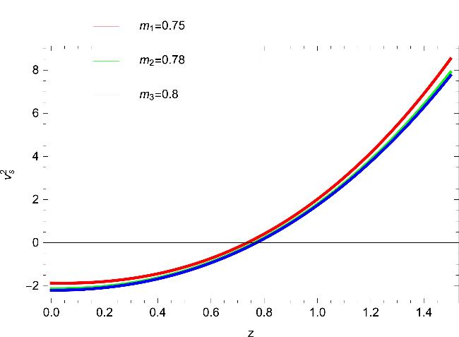
Figure 11. Plot of ${v}_{s}^{2}$ for intermediate scale factor. |
3.3. Two unified phases scale factor
In this section, we consider the two unified phases scale factor which unifies the matter-dominate phase to accelerated phase. We apply the reconstruction technique to obtain a reconstructed function f(Q). The Hubble parameter for two unified phases scale factor, can be written as 11 ) and (23 ) and find the reconstructed function f(Q) which is written as follows:
$\begin{eqnarray}\begin{array}{r}H(t)={H}_{1}+{H}_{2}/t;\end{array}\end{eqnarray}$
The scale factor a(t) can be written in term of Hubble parameter as: $\begin{eqnarray}a(t)=b{{\rm{e}}}^{{H}_{1}t}{t}^{{H}_{2}}.\end{eqnarray}$
When t is very small, we have H(t) ∼ H2/t, indicating the presence of a perfect fluid in the Universe with an EoS parameter written as ω = −1 + 2/3H2. Conversely, a constant Hubble parameter is implied by H → H1 when t is very large. The de Sitter universe is thus represented by H(t), which offers a transition from a matter-dominated to an accelerating phase. In this work, we use the reconstruction technique to find the reconstructed function. We equate equations ( $\begin{eqnarray*}\begin{array}{rcl}f(Q) & = & \left(3{c}^{2}{\left(\frac{{H}_{2}}{t}+{H}_{1}\right)}^{2}((\pi \delta +(({H}_{2})({t}^{-1})\right.\\ & & \left.{\left.+{H}_{1}){)}^{2}){\left({\left(\frac{{H}_{2}}{t}+{H}_{1}\right)}^{2}\right)}^{-1}\right)}^{R/\delta }-1\right)\\ & & \times {(4\pi R)}^{-1}+\sqrt{{\rm{e}}}{c}_{1}.\end{array}\end{eqnarray*}$
Figure 12 shows the reconstructed function against redshift parameter 0 < z < 1.5. It can be seen in figure 12 that the trajectories represent increasing behavior for H2 = 2, 2.3, 2.5 and H1 = 0.9. The values of other parameters are: δ = 0.5, R = 0.8, c = 13, g = 2.2 and c1 = 0.8. All three trajectories show that when the value of H2 increases, the reconstructed function f(Q) is decreasing.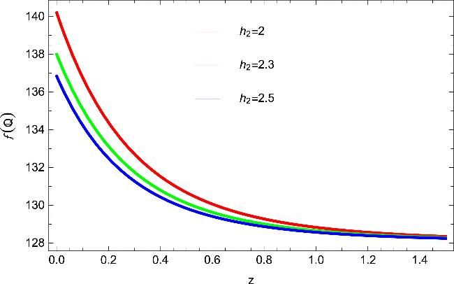
Figure 12. Plot of reconstructed function f(Q) for unification of two phases scale factor. |
Next, we find the EoS parameter for unification scale factor by using equations (23 ) and (24 ). The EoS parameter for unification scale factor is:
$\begin{eqnarray*}\begin{array}{rcl}\omega & = & \left(8{\left(\frac{{\left({H}_{1}t+{H}_{2}\right)}^{2}}{{t}^{2}}\right)}^{n}\left(\left(\left(n-\frac{1}{2}\right){H}_{1}^{3}\right.\right.\right.\\ & & \left.+\frac{{n}^{2}}{18}-\frac{n}{18}\right){t}^{3}\\ & & +3{H}_{1}^{2}{H}_{2}\left(n-\frac{1}{2}\right){t}^{2}+3{H}_{1}\left(\left(n-\frac{1}{2}\right){H}_{2}\right.\\ & & -\left.\left.\frac{n}{9}\right){H}_{2}t+\left(\left(n-\frac{1}{2}\right){H}_{2}-\frac{n}{3}\right){H}_{2}^{2}\right)\\ & & \times \left.\pi {t}^{4}{6}^{n}R\alpha \right)\left(3{c}^{2}{\left({H}_{1}t+{H}_{2}\right)}^{7}\right.\\ & & \times {\left.\left({\left(\frac{\left(\pi \delta +{H}_{1}^{2}\right){t}^{2}+2t{H}_{1}{H}_{2}+{H}_{2}^{2}}{{\left({H}_{1}t+{H}_{2}\right)}^{2}}\right)}^{\frac{R}{\delta }}-1\right)\right)}^{-1}.\end{array}\end{eqnarray*}$
The graph of EoS parameter ω is shown in figure 13. The EoS parameter ω exhibits an increasing behavior with redshift. At low redshift it lies in the non-phantom region, then crosses the phantom divide as z increases, and finally evolves toward the quintessence region at higher redshift.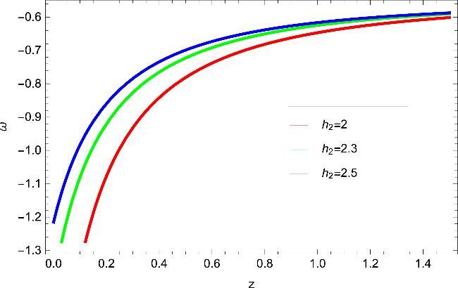
Figure 13. Plot of EoS parameter ω for unification of two phases scale factor. |
Next, we obtain the deceleration parameter q by using equations (16 ) and (18 ), written as:
The deceleration parameter q is shown in figure 14, displays a similar evolutionary trend to the EoS parameter, indicating a consistent dynamical behavior of the reconstructed model. As ω transitions between different dark energy regimes, the corresponding shift in q reflects a smooth evolution from a decelerated phase to an accelerated one. Now, we take the derivative of equation (18 ) to get the ${\omega }^{{\prime} }$ which is as follows:
$\begin{eqnarray*}\begin{array}{rcl}{\omega }^{{\prime} } & = & -\left(16{t}^{3}{6}^{n}\alpha {\left(\frac{{\left({H}_{1}t+{H}_{2}\right)}^{2}}{{t}^{2}}\right)}^{n}R\pi \right.\\ & & \times \left(\left(\left(\left(\frac{{H}_{1}^{2}}{18}+\frac{\pi \delta }{18}\right){n}^{3}\right.\right.\right.\\ & & +\left({H}_{1}^{5}+\pi \delta {H}_{1}^{3}-\frac{{H}_{1}^{2}}{4}+\frac{\left(R-\frac{9\delta }{2}\right)\pi }{18}\right){n}^{2}\\ & & +\left(-\frac{5{H}_{1}^{5}}{2}+\pi \left(R-\frac{5\delta }{2}\right){H}_{1}^{3}\right.\\ & & +\left.\frac{7{H}_{1}^{2}}{36}-\frac{\pi \left(R-\frac{7\delta }{2}\right)}{18}\right)n\\ & & -\left.\frac{{H}_{1}^{3}\left(-2{H}_{1}^{2}+\pi \left(R-2\delta \right)\right)}{2}\right){t}^{5},\end{array}\end{eqnarray*}$
$\begin{eqnarray*}\begin{array}{rcl} & & +3\left(\frac{{n}^{3}{H}_{2}}{27}+{H}_{2}\left(\pi \delta {H}_{1}+\frac{5}{3}{H}_{1}^{3}-\frac{1}{6}\right){n}^{2}\right.\\ & & +\left(\left(\frac{7}{54}-\frac{25{H}_{1}^{3}}{6}+\pi \left(R-\frac{5\delta }{2}\right){H}_{1}\right){H}_{2}\right.\\ & & -\left.\frac{{H}_{1}\left(\pi \delta +{H}_{1}^{2}\right)}{9}\right)n\\ & & -\left.\frac{\left(-\frac{10{H}_{1}^{2}}{3}+\pi \left(R-2\delta \right)\right){H}_{2}{H}_{1}}{2}\right){H}_{1}{t}^{4}\\ & & +3{H}_{2}\left(\frac{{n}^{3}{H}_{2}}{54}+\left(\left(\pi \delta {H}_{1}+\frac{10}{3}{H}_{1}^{3}-\frac{1}{12}\right)\right.\right.\\ & & \left.\times {H}_{2}-\frac{{H}_{1}\left(\pi \delta +{H}_{1}^{2}\right)}{9}\right){n}^{2}\\ & & +\left(\left(\frac{7}{108}-\frac{25{H}_{1}^{3}}{3}+\pi \left(R-\frac{5\delta }{2}\right){H}_{1}\right)\right.\end{array}\end{eqnarray*}$
$\begin{eqnarray*}\begin{array}{rcl} & & \left.\times {H}_{2}-\frac{\left({H}_{1}^{2}+\pi \left(R-\delta \right)\right){H}_{1}}{9}\right)n\\ & & -\left.\frac{\left(-\frac{20{H}_{1}^{2}}{3}+\pi \left(R-2\delta \right)\right){H}_{2}{H}_{1}}{2}\right){t}^{3}\\ & & +{H}_{2}^{2}\left(\left(\left(\pi \delta +10{H}_{1}^{2}\right){H}_{2}-{H}_{1}^{2}-\frac{\pi \delta }{3}\right){n}^{2}\right.\\ & & +\left(\left(-25{H}_{1}^{2}+\pi \left(R-\frac{5\delta }{2}\right)\right){H}_{2}\right.\\ & & \left.+{H}_{1}^{2}-\frac{\pi \left(R-2\delta \right)}{3}\right)n\\ & & -\left.\frac{\left(-20{H}_{1}^{2}+\pi \left(R-2\delta \right)\right){H}_{2}}{2}\right){t}^{2}+5{H}_{2}^{3}\left(\left({H}_{2}\right.\right.\end{array}\end{eqnarray*}$
$\begin{eqnarray*}\begin{array}{rcl} & & \left.\left.-\frac{1}{5}\right){n}^{2}+\left(-\frac{5{H}_{2}}{2}+\frac{1}{3}\right)n+{h}_{2}\right)\\ & & \times {H}_{1}t+\left(n-2\right){H}_{2}^{4}\left(\left({H}_{2}-\frac{1}{3}\right)n-\frac{{H}_{2}}{2}\right))\\ & & \times {\left(\frac{\left(\pi \delta +{H}_{1}^{2}\right){t}^{2}+2t{H}_{1}{H}_{2}+{H}_{2}^{2}}{{\left({H}_{1}t+{H}_{2}\right)}^{2}}\right)}^{\frac{R}{\delta }}\\ & & -\left(\left(\pi \delta +{H}_{1}^{2}\right){t}^{2}+2t{H}_{1}{H}_{2}+{H}_{2}^{2}\right)\left(\left(\frac{{n}^{3}}{18}\right.\right.\\ & & +\left.\left({H}_{1}^{3}-\frac{1}{4}\right){n}^{2}+\left(-\frac{5{H}_{1}^{3}}{2}+\frac{7}{36}\right)n+{H}_{1}^{3}\right){t}^{3}\\ & & +3\left({n}^{2}{H}_{2}+\left(-\frac{5{H}_{2}}{2}-\frac{1}{9}\right)n+{H}_{2}\right){H}_{1}^{2}{t}^{2}\\ & & +3\left(\left({H}_{2}-\frac{1}{9}\right){n}^{2}+\left(-\frac{5{h}_{2}}{2}+\frac{1}{9}\right)n+{h}_{2}\right)\\ & & \times {H}_{2}{H}_{1}t+\left(n-2\right)\end{array}\end{eqnarray*}$
$\begin{eqnarray*}\begin{array}{rcl} & & \times \left.\left.{H}_{2}^{2}\left(\left({H}_{2}-\frac{1}{3}\right)n-\frac{{H}_{2}}{2}\right)\right)){H}_{2}\right)\\ & & \times \left(3\left(\left(\pi \delta +{H}_{1}^{2}\right){t}^{2}+2t{H}_{1}{H}_{2}+{H}_{2}^{2}\right)\right.\\ & & \times {\left({\left(\frac{\left(\pi \delta +{H}_{1}^{2}\right){t}^{2}+2t{H}_{1}{H}_{2}+{H}_{2}^{2}}{{\left({H}_{1}t+{H}_{2}\right)}^{2}}\right)}^{\frac{R}{\delta }}-1\right)}^{2}\\ & & \times {\left.{c}^{2}{\left({H}_{1}t+{H}_{2}\right)}^{8}\right)}^{-1}\end{array}\end{eqnarray*}$
and represent the graph of $\omega -{\omega }^{{\prime} }$ phase plane in figure 15. In this figure, $\omega -{\omega }^{{\prime} }$ phase plane shows the freezing region of the Universe. Also, we find the statefinder parameter r − s and find the behavior of SMHDE model.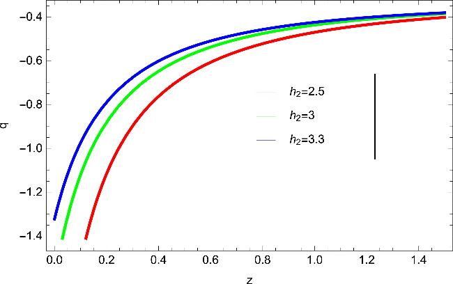
Figure 14. Plot of deceleration parameter q for unification of two phases scale factor. |
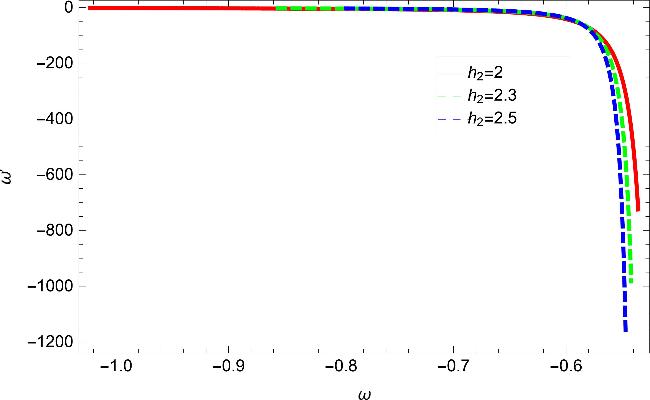
Figure 15. Plot of $\omega -{\omega }^{{\prime} }$ plane for unification of two phases scale factor. |
For this, we take equation (18 ) and (23 ), we get our jerk parameter r
$\begin{eqnarray*}\begin{array}{rcl}r & = & \left(81(\left(\pi \delta +{H}_{1}^{2}\right){t}^{2}+2t{H}_{1}{H}_{2}\right.\\ & & +{H}_{2}^{2}){c}^{4}{\left({H}_{1}t+{H}_{2}\right)}^{14}\left(((\left(\pi \delta +{H}_{1}^{2}\right){t}^{2}\right.\\ & & {\left.\times +2t{H}_{1}{H}_{2}+{H}_{2}^{2}){\left({\left({H}_{1}t+{H}_{2}\right)}^{2}\right)}^{-1}{)}^{\frac{R}{\delta }}\right)}^{2}\\ & & +648{c}^{2}{\left({H}_{1}t+{H}_{2}\right)}^{6}\left({t}^{3}\right.\\ & & \times \left(\frac{{t}^{3}\left(\left(\pi \delta +{H}_{1}^{2}\right){t}^{2}+2t{H}_{1}{H}_{2}+{H}_{2}^{2}\right)n{H}_{2}{6}^{n-1}}{2}\right.\\ & & +\left(\left({H}_{1}\left(\left(18n-9\right){H}_{1}^{3}+{n}^{2}-n\right)\left(\pi \delta +{H}_{1}^{2}\right){t}^{7}\right)\right.\\ & & \times {(12)}^{-1}+((\left(\left(72n-36\right){H}_{1}^{3}+{n}^{2}-n\right)\delta \pi \\ & & +3{H}_{1}^{2}\left(\left(36n-18\right){H}_{1}^{3}+{n}^{2}-n\right)){H}_{2}{t}^{6}){(12)}^{-1}\\ & & \times +\left(\left(\left(9{H}_{1}\left(36{H}_{1}\delta \left(n-\frac{1}{2}\right)\pi \right.\right.\right.\right.\\ & & +\left.\left.\left(90n-45\right){H}_{1}^{3}+{n}^{2}-n\right){H}_{2}\right)\frac{1}{2}\\ & & +\left(18\left(n-\frac{1}{2}\right)\left(R+\delta \left(n-2\right)\right){H}_{1}^{3}-9n\delta {H}_{1}^{2}\right.\\ & & +\left.\left(\left(n-1\right)R+\left(n-4\right)\delta \left(n-\frac{1}{2}\right)\right)n\right)\pi \\ & & +{H}_{1}^{2}\left(\left(18{n}^{2}-45n+18\right){H}_{1}^{3}\right.,\end{array}\end{eqnarray*}$
$\begin{eqnarray*}\begin{array}{rcl} & & \left.\left.\left.-9n{H}_{1}^{2}+{n}^{3}-\frac{9{n}^{2}}{2}+2n\right)\right){H}_{2}{t}^{5}\right){(18)}^{-1}\\ & & +3\left(\left(2{H}_{1}\delta \left(n-\frac{1}{2}\right)\pi +\left(10n-5\right){H}_{1}^{3}\right.\right.\\ & & +\left.\frac{{n}^{2}}{36}-\frac{n}{36}\right){H}_{2}^{2}+{H}_{1}\left(\left(\left(n-\frac{1}{2}\right)\right.\right.\\ & & \left.\times \left(R+\delta \left(n-2\right)\right){H}_{1}-\frac{n\delta }{3}\right)\pi +\left(\frac{5}{3}{n}^{2}\right.\\ & & -\left.\frac{25}{6}n+\frac{5}{3}\right){H}_{1}^{3}-\frac{2n{H}_{1}^{2}}{3}+\frac{{n}^{3}}{27}-\frac{{n}^{2}}{6}\\ & & +\left.\left.\frac{2n}{27}\right){H}_{2}-\frac{n{H}_{1}^{2}\left(\pi \delta +{H}_{1}^{2}\right)}{9}\right){H}_{2}{t}^{4}\\ & & +3\left(\frac{\left(n-\frac{1}{2}\right)\left(\pi \delta +15{H}_{1}^{2}\right){H}_{2}^{2}}{2}\right.\\ & & +\left(\left(\left(n-\frac{1}{2}\right)\left((R+\delta \left(n-2\right)){H}_{1}-\frac{n\delta }{6}\right)\pi \right.\right.\\ & & +\left(\frac{10}{3}{n}^{2}-\frac{25}{3}n+\frac{10}{3}\right){H}_{1}^{3}-n{H}_{1}^{2}\\ & & +\left.\frac{{n}^{3}}{54}-\frac{{n}^{2}}{12}+\frac{n}{27}\right){H}_{2}\end{array}\end{eqnarray*}$
$\begin{eqnarray*}\begin{array}{rcl} & & \left.-\left({H}_{1}\left(\left(n\delta +R-\delta \right)\pi +{H}_{1}^{2}\left(n+1\right)\right)n\right)\frac{1}{9}\right)\\ & & \times {H}_{2}^{2}{t}^{3}+{H}_{2}^{3}(9{H}_{1}\left(n-\frac{1}{2}\right){H}_{2}^{2}\\ & & +\left(\left(n-\frac{1}{2}\right)\left(R+\delta \left(n-2\right)\right)\pi \right.\\ & & +\left.10{H}_{1}\left(\left({n}^{2}-\frac{5}{2}n+1\right){H}_{1}-\frac{n}{5}\right)\right){H}_{2}\\ & & -\left(n\left(\left(n\delta +R-2\delta \right)\pi +3{H}_{1}^{2}\left(n-1\right)\right)\right)\frac{1}{3}){t}^{2}\\ & & +\left(3\left(\left(n-\frac{1}{2}\right){H}_{2}^{2}+\left(\left(\frac{10}{3}{n}^{2}-\frac{25}{3}n+\frac{10}{3}\right)\right.\right.\right.\end{array}\end{eqnarray*}$
$\begin{eqnarray*}\begin{array}{rcl} & & \times \left.\left.\left.{H}_{1}-\frac{n}{3}\right){H}_{2}-\frac{2{H}_{1}n\left(n-\frac{5}{3}\right)}{3}\right){H}_{2}^{4}t\right)\\ & & \times \frac{1}{2}+\left(n-2\right)\left(\left(n-\frac{1}{2}\right){H}_{2}-\frac{n}{3}\right)\\ & & \times \left.\left.{H}_{2}^{5}\right){6}^{n}\right)\alpha R\pi {\left(\frac{{\left({H}_{1}t+{H}_{2}\right)}^{2}}{{t}^{2}}\right)}^{n}\\ & & -\left(\left(\left(\pi \delta +{H}_{1}^{2}\right){t}^{2}+2t{H}_{1}{H}_{2}+{H}_{2}^{2}\right){c}^{2}\right.\\ & & \times \left.\left.{\left({H}_{1}t+{H}_{2}\right)}^{8}\right)\frac{1}{4}\right)\\ & & \times {\left(\frac{\left(\pi \delta +{H}_{1}^{2}\right){t}^{2}+2t{H}_{1}{H}_{2}+{H}_{2}^{2}}{{\left({H}_{1}t+{H}_{2}\right)}^{2}}\right)}^{\frac{R}{\delta }}\end{array}\end{eqnarray*}$
$\begin{eqnarray*}\begin{array}{rcl} & & +2592\left(\left(\pi \delta +{H}_{1}^{2}\right){t}^{2}+2t{H}_{1}{H}_{2}+{H}_{2}^{2}\right)\\ & & \times \left({t}^{8}{\alpha }^{2}{\left({6}^{n}\right)}^{2}{R}^{2}\left(\left(\left(n-\frac{1}{2}\right){H}_{1}^{3}+\frac{{n}^{2}}{18}\right.\right.\right.\\ & & -\left.\frac{n}{18}\right){t}^{3}+3{H}_{1}^{2}\left(n-\frac{1}{2}\right){H}_{2}{t}^{2}\\ & & +3\left(\left(n-\frac{1}{2}\right){H}_{2}-\frac{n}{9}\right){H}_{1}{H}_{2}t+{H}_{2}^{2}\\ & & {\left.\times \left(\left(n-\frac{1}{2}\right){H}_{2}-\frac{n}{3}\right)\right)}^{2}{\pi }^{2}{\left({\left(\frac{{\left({H}_{1}t+{H}_{2}\right)}^{2}}{{t}^{2}}\right)}^{n}\right)}^{2}\\ & & -\left({t}^{3}\alpha {c}^{2}{\left({H}_{1}t+{H}_{2}\right)}^{6}\left(\frac{{H}_{2}{6}^{n-1}n\,{t}^{3}}{2}\right.\right.\\ & & +\left(\frac{{H}_{1}\left(\left(18n-9\right){H}_{1}^{3}+{n}^{2}-n\right){t}^{5}}{12}\right.\\ & & +\left(\left(\left(72n-36\right){H}_{1}^{3}+{n}^{2}-n\right){H}_{2}{t}^{4}\right)\frac{1}{12}\end{array}\end{eqnarray*}$
$\begin{eqnarray*}\begin{array}{rcl} & & +9\left({H}_{1}^{2}\left(n-\frac{1}{2}\right){H}_{2}+\left(\frac{1}{9}{n}^{2}-\frac{5}{18}n+\frac{1}{9}\right){H}_{1}^{3}\right.\\ & & -\left.\frac{n{H}_{1}^{2}}{18}+\frac{{n}^{3}}{162}-\frac{{n}^{2}}{36}+\frac{n}{81}\right){H}_{2}{t}^{3}\\ & & +6{H}_{1}\left(\left(n-\frac{1}{2}\right){H}_{2}^{2}+\left(\left(\frac{1}{2}{n}^{2}\right.\right.\right.\\ & & -\left.\left.\frac{5}{4}n+\frac{1}{2}\right){H}_{1}-\frac{n}{6}\right)\\ & & \times \left.{H}_{2}-\frac{n{H}_{1}}{18}\right){H}_{2}{t}^{2}+\left(3\left(\left(n-\frac{1}{2}\right)\right.\right.\\ & & \times {H}_{2}^{2}+\left(\left(2{n}^{2}-5n+2\right){H}_{1}-\frac{n}{3}\right){H}_{2}\\ & & -\left.\left.\frac{2n{H}_{1}\left(n-1\right)}{9}\right){H}_{2}^{2}t\right)\frac{1}{2}+\left(n-2\right)\\ & & \times \left.\left.\left(\left(n-\frac{1}{2}\right){H}_{2}-\frac{n}{3}\right){H}_{2}^{3}\right){6}^{n}\right)R\pi \left(\left(\left({H}_{1}t\right.\right.\right.\end{array}\end{eqnarray*}$
$\begin{eqnarray*}\begin{array}{rcl} & & \left.\left.\left.{\left.\left.{\left.+{H}_{2}\right)}^{2}\right){t}^{-2}\right)}^{n}\right)\frac{1}{4}+\frac{{c}^{4}{\left({H}_{1}t+{H}_{2}\right)}^{14}}{32}\right)\right)\\ & & \times \left(81\left(\left(\pi \delta +{H}_{1}^{2}\right){t}^{2}+2t{H}_{1}{H}_{2}\right.\right.\\ & & +\left.{H}_{2}^{2}\right){c}^{4}{\left({H}_{1}t+{H}_{2}\right)}^{14}\\ & & \times {\left.{\left({\left(\frac{\left(\pi \delta +{H}_{1}^{2}\right){t}^{2}+2t{H}_{1}{H}_{2}+{H}_{2}^{2}}{{\left({H}_{1}t+{H}_{2}\right)}^{2}}\right)}^{\frac{R}{\delta }}-1\right)}^{2}\right)}^{-1}\end{array}\end{eqnarray*}$
and snap parameter s and display its graphical representation in figure 16. In the r-s plane, the trajectory begins in the negative s region with r close to unity, and the parameter s increases monotonically toward the positive domain. As s crosses zero, the statefinder parameter r exhibits only a very slight deviation from the ΛCDM value, remaining extremely close to r = 1 throughout the evolution. Overall, the r − s trajectory shows an evolution from a non-ΛCDM regime in the negative-s region toward the vicinity of the fixed point (r = 1, s = 0). The parameter r remains almost constant and very close to unity, indicating that the model stays near the ΛCDM behavior throughout its evolution. This confirms that the reconstructed scenario tends asymptotically toward a ΛCDM-like phase at late times.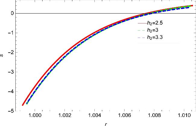
Figure 16. Plot of r − s plane for two unified phases scale factor. |
After this, we find the speed square of sound parameter for unification scale factor which is as follows:
$\begin{eqnarray*}\begin{array}{rcl}{v}_{{\rm{s}}}^{2} & = & -\left(27\left(\left(\left(-2{H}_{1}^{2}+\pi \left(R-2\delta \right)\right){t}^{2}\right.\right.\right.\\ & & \left.-4t{H}_{1}{H}_{2}-2{H}_{2}^{2}\right)\left(\left(\left(\pi \delta +{H}_{1}^{2}\right){t}^{2}\right.\right.\\ & & +{\left.\left.2t{H}_{1}{H}_{2}+{H}_{2}^{2}\right){\left({\left({H}_{1}t+{H}_{2}\right)}^{2}\right)}^{-1}\right)}^{\frac{R}{\delta }}\\ & & +\left.\left.\left(2\pi \delta +2{H}_{1}^{2}\right){t}^{2}+4t{H}_{1}{H}_{2}+2{H}_{2}^{2}\right)\right)\\ & & \times \left.{\left({H}_{1}t+{H}_{2}\right)}^{7}{c}^{2}{6}^{-n}{\left(\frac{{\left({H}_{1}t+{H}_{2}\right)}^{2}}{{t}^{2}}\right)}^{-n}\right)\\ & & \times \left(2{t}^{4}\alpha n\left((36{H}_{1}^{3}+n-1){t}^{3}\right.\right.\\ & & +108{H}_{1}^{2}\left({H}_{2}-\frac{1}{9}\right){t}^{2}\\ & & +\left.108{H}_{2}\left({H}_{2}-\frac{2}{9}\right){H}_{1}t+36{H}_{2}^{3}-12{H}_{2}^{2}\right)\\ & & \times {\left.\left(\left(\pi \delta +{H}_{1}^{2}\right){t}^{2}+2t{H}_{1}{H}_{2}+{H}_{2}^{2}\right)R\pi \right)}^{-1}\end{array}\end{eqnarray*}$
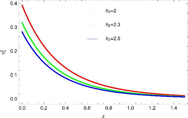
Figure 17 shows the stable behavior for two unified phases scale factor.
Figure 17. Plot of ${v}_{0}^{s}$ plane for two unified phases scale factor. |
4. Conclusion
In this work, we have successfully reconstructed the SMHDE model within the framework of f(Q) gravity, a modified gravity theory based on the non-metricity scalar Q. The reconstruction was carried out in a spatially flat Friedmann-Lemaître–Robertson-Walker (FLRW) background, employing Sharma-Mittal entropy as a generalized, non-extensive entropy measure. This approach enabled us to investigate the influence of non-additive thermodynamic properties on the evolution of dark energy in a modified gravity context.
To examine the cosmological viability of the reconstructed model, we analyzed several key dynamical and diagnostic parameters, including the EoS parameter ω, the deceleration parameter q, the $\omega -{\omega }^{{\prime} }$ plane, the statefinder parameters (r, s), and the squared speed of sound ${v}_{{\rm{s}}}^{2}$.
Our main findings can be summarized as follows:
The region with ω≥ −1 corresponds to the non-phantom regime, which includes quintessence-like behavior for $-1\lt \omega \lt -\frac{1}{3}$ and the cosmological constant boundary at ω = −1.
The deceleration parameter q demonstrates a smooth transition from a decelerating to an accelerating phase, consistent with the late-time acceleration of the Universe.
The analysis of the $\omega -{\omega }^{{\prime} }$ plane places the model within stable regions associated with freezing and thawing dark energy scenarios.
The statefinder diagnostic (r, s) shows that the SMHDE model deviates from the standard ΛCDM trajectory, while still remaining within the bounds allowed by observational data, thus offering a distinguishable but viable cosmological signature.
The squared speed of sound ${v}_{{\rm{s}}}^{2}$ remains non-negative under suitable parameter conditions, implying classical stability of the model.
Overall, the SMHDE model reconstructed in f(Q) gravity presents a consistent and observationally supported description of dark energy. The model exhibits flexibility through its two entropy parameters and successfully recovers Tsallis and Rényi HDE models in limiting cases. Its ability to account for phantom behavior and dynamically stable cosmic evolution makes it a promising candidate for explaining the accelerated expansion of the Universe.
Future work may involve confronting the model with observational data sets such as Type Ia supernovae, CMB, and BAO, as well as studying perturbation growth and structure formation to further assess the robustness of the proposed framework.
Hence, the overall dynamics of the Universe's expansion is impacted by changes in the scale factor. However, in our work, the EoS parameter ω, the deceleration parameter q shifts from positive to negative indicating the transition from deceleration to acceleration for all scale factors. In a freezing scenario, the DE behaves like a cosmological constant and evolves towards ω = −1, whereas in a thawing scenario, it begins with a more complex form and progressively approaches ω = −1. These models hold great significance for comprehending the Universe's expansion and the part DE will play in its future.