


1. Introduction
Modifying general relativity (GR) to address unresolved problems such as the cosmological constant and dark matter has become a common approach. Lovelock's theorem shows that GR is the unique metric theory in four dimensions whose equations of motion are second order, local, and invariant under spacetime diffeomorphism [1]. Consequently, any modification of GR must violate at least one of these assumptions, for instance by introducing extra fields (as in scalar-tensor theories), new geometric structures (such as non-Riemannian geometry), higher dimensions, or higher-order derivatives. Among these possibilities, scalar-tensor theories have seen remarkable progress in the past two decades, especially in the construction of higher-derivative models [2–6]. However, single-field scalar-tensor theories with second-order derivatives are now strongly constrained by observations, including those concerning the propagation speed of gravitational waves [7–12].
A natural alternative is to introduce vector fields. Indeed, all fundamental forces in the Standard Model are mediated by vector fields, which motivates exploring their role in cosmology beyond scalar degrees of freedom (DOFs). Inspired by the success of constructing higher derivative scalar-tensor theories, vector field theories with at most second-order equations of motion have been developed [13] and generalized to curved spacetimes under the name generalized Proca theory [14] (see also [15]). The generalized Proca theory has been extensively studied in cosmology [16–20], in black hole physics [21–26] and in the context of gravitational waves [27–29]. See also [30] for a review and more references therein. The generalized Proca theory has been further generalized to the so-called extended vector-tensor theory, which relies on the degeneracy of higher order derivatives rather than restricting the order of the equations of motion [31–37].
A no-go theorem [38] forbids the Galileon-type interactions of vector fields in flat spacetime if both Lorentz invariance and U(1) gauge invariance are preserved. Indeed, in generalized Proca theory and extended vector-tensor theory, U(1) invariance is explicitly broken. Nevertheless, progress has been made in constructing Einstein–Maxwell theories that retain U(1) symmetry [39–41]. Generally, once U(1) invariance is broken, the vector sector propagates three DOFs: two transverse polarization modes and an additional longitudinal mode.
The purpose of this work is to ask a basic question: is it possible to construct a vector field theory that propagates only the two transverse DOFs3 ? Clearly, enforcing both Lorentz invariance and U(1) invariance recovers the Maxwell theory for a free vector field. Therefore, to explore possible generalizations, we relax these symmetries and require only spatial covariance, without assuming U(1) invariance. As a first step, we neglect gravitational effects and work in flat spacetime. This setup can be viewed as a local limit of a foliated cosmological spacetime. Locally the metric is approximately flat on scales much smaller than the curvature scale, while a cosmological evolution can still motivate a preferred time slicing and hence the breaking of time diffeomorphisms. The relevant constraint structure in the vector sector can still be captured in this setup. The analysis in this work therefore serves as a ‘decoupling limit' of the theory with gravitational effects.
This flat-background analysis should be viewed as a controlled limit of a preferred-foliation cosmological setting: locally (or in the high-frequency/decoupling regime) the background metric can be approximated by Minkowski while the reduced symmetry structure—spatial covariance with broken time diffeomorphisms—still captures the relevant constraint mechanism in the vector sector.
In the context of the generalized Proca theory, the Faddeev–Jackiw formalism has been applied to count the number of DOFs [45]. The so-called Maxwell–Proca theory proposed in [46, 47] shows that a vector field propagating two DOFs corresponds to a real Abelian vector field whose Lagrangian involves two first-class constraints. This naturally raises the question of whether one can construct a more general flat-spacetime vector field theory that still propagates two DOFs but involves additional second-class constraints. The present work is devoted to exploring this question.
The remainder of the paper is organized as follows. In section 2 , we introduce our model of vector field theory respecting only the spatial invariance. In section 3 we set up our formalism for the Hamiltonian constraint analysis and show that generally the theory propagates three DOFs. In section 4 , we derive the first degeneracy condition in order to reduce the number of DOFs. In section 5 is devoted to the second degeneracy condition, which is necessary in order to fully reduce the number of DOFs from three to two. In section 6 , we summarize our results.
2. The spatially covariant vector field theory
Our purpose is to construct a vector field theory respecting only spatial covariance. In this work, we neglect the gravitational effects and consider a flat spacetime background, where the metric is
$\begin{eqnarray}{\rm{d}}{s}^{2}=-{\rm{d}}{t}^{2}+{\delta }_{ij}{\rm{d}}{x}^{i}{\rm{d}}{x}^{j}.\end{eqnarray}$
That is, we treat the vector field Aμ as a test field in a fixed flat background.The global Lorentz symmetry is explicitly broken, and we retain only the subgroup of spatial rotations SO(3). Accordingly, we decompose the vector field into its temporal and spatial components,
$\begin{eqnarray}{A}_{\mu }=\left({A}_{0},{A}_{i}\right),\end{eqnarray}$
where i, j = 1, 2, 3 are spatial indices. Since Lorentz symmetry is broken, the usual electromagnetic tensor Fμν with components $\begin{eqnarray}{F}_{0i}={\dot{A}}_{i}-{\partial }_{i}{A}_{0},\,{F}_{ij}={\partial }_{i}{A}_{j}-{\partial }_{j}{A}_{i},\end{eqnarray}$
is no longer a preferred object. Instead, the Lagrangian can be a general function of the first derivatives of the vector field. From this perspective, the Maxwell theory corresponds to a particular combination of quadratic monomials in the first derivatives of the vector field.The most general spatially covariant Lagrangian takes the schematic form ${ \mathcal L }\left({A}_{0},{A}_{i},{\partial }_{t},{\partial }_{i}\right).$ In this work, we restrict ourselves to Lagrangians that are polynomials in the derivative terms Each monomial is constructed from spatial scalar formed by contracting the vector field and its first order derivatives
$\begin{eqnarray}{\dot{A}}_{0},\,{\partial }_{i}{A}_{0},\,{\dot{A}}_{i},\,{\partial }_{i}{A}_{j},\end{eqnarray}$
where an over-dot denotes a time derivative.We will construct and classify possible monomials according to the total number of derivatives. In this work, we focus on Lagrangians up to the quadratic order in derivatives. That is, the total number of derivatives in each monomial in the Lagrangian is at most two.
At the zeroth order in derivatives, the two basic spatial scalars are $\bar{X}\equiv {A}_{i}{A}^{i}$ and A0. The corresponding Lagrangian is therefore an arbitrary function of these two quantities, i.e.
$\begin{eqnarray}{{ \mathcal L }}_{2}={f}_{2}({A}_{0},\bar{X}).\end{eqnarray}$
In this work we choose the subscripts of ${{ \mathcal L }}_{n}$ following the notation used in Horndeski and generalized Proca theories [4, 5, 14]4 .At linear order in derivatives, there are five scalar contractions:
$\begin{eqnarray*}{\dot{A}}_{0},\,{A}^{i}{\partial }_{i}{A}_{0},\,{A}^{i}{\dot{A}}_{i},\,{\partial }_{i}{A}^{i},\,{A}^{i}{A}^{j}{\partial }_{i}{A}_{j}.\end{eqnarray*}$
In this work, we require that contractions occur only among derivative terms themselves. Terms involving contractions between derivatives and the undifferentiated vector field, such as Ai∂iA0, ${A}^{i}{\dot{A}}_{i}$ and AiAj∂iAj will not be considered. This restriction is primarily adopted for tractability and for isolating the degeneracy structure in the simplest nontrivial operator basis. Allowing additional operators (such as Ai∂iA0, ${A}^{i}{\dot{A}}_{i}$ or AiAj∂iAj) enlarges the basis substantially and in general modifies the momentum dependence of the primary constraint and the subsequent constraint chain, so that additional degeneracy conditions may be required to eliminate the longitudinal mode. The Hamiltonian strategy developed in this work can in principle be extended to the fully general basis, but the systematic classification becomes considerably broader. The present work therefore focuses on the above minimal class to obtain explicit, classifiable two-DOF theories. With this assumption, we are left with two admissible monomials, ${\dot{A}}_{0}$ and ∂iAi, and the Lagrangian is given by $\begin{eqnarray}{{ \mathcal L }}_{3}={f}_{3,1}{\dot{A}}_{0}+{f}_{3,2}{\partial }_{i}{A}^{i},\end{eqnarray}$
where coefficients f3,1 and f3,2 are general functions of A0 and $\overline{X}$.As quadratic order in derivatives, one can form a large number of scalar monomials by contracting indices of ${\dot{A}}_{0}$, ∂iA0, ${\dot{A}}_{i}$ and ∂iAj. We find ten types of monomial. The complete set of scalar monomials can be classified as:
${\left({\dot{A}}_{0}\right)}^{2}$
${A}^{i}{\dot{A}}_{0}{\partial }_{i}{A}_{0}$
${\dot{A}}_{0}{\dot{A}}_{i}{A}^{i}$
${\dot{A}}_{0}{\partial }_{i}{A}^{i}$, ${\dot{A}}_{0}{\partial }_{i}{A}_{j}{A}^{i}{A}^{j}$
∂iA0∂iA0, AiAj∂jA0∂iA0
${\partial }^{i}{A}_{0}{\dot{A}}_{i}$, ${A}^{i}{A}^{j}{\partial }_{j}{A}_{0}{\dot{A}}_{i}$
Ak∂kA0∂iAi, Ai∂jA0∂iAj, Aj∂iA0∂iAj, AkAiAj∂kA0∂iAj
${\dot{A}}_{i}{\dot{A}}^{i}$, ${A}^{i}{A}^{j}{\dot{A}}_{j}{\dot{A}}_{i}$
${A}^{k}{\dot{A}}_{k}{\partial }_{i}{A}^{i}$, ${A}^{i}{\dot{A}}^{j}{\partial }_{i}{A}_{j}$, ${A}^{j}{\dot{A}}^{i}{\partial }_{i}{A}_{j}$, ${A}^{k}{A}^{i}{A}^{j}{\dot{A}}_{k}{\partial }_{i}{A}_{j}$
∂iAi∂jAj, ∂iAj∂iAj, ∂iAj∂jAi, AiAj∂kAk∂iAj, AiAj∂kAi∂kAj, AiAj∂kAi∂jAk, AiAj∂iAk∂jAk, AiAjAkAl∂iAj∂kAl.
As in the case of the linear order, if we impose the same restriction that contractions must occur only among derivative terms, we are left with the following eight contractions 2.7 ), we denote the corresponding coefficients by hm,n purely for notational convenience. No physical distinction is implied: all fm,n and hm,n are general functions of A0 and $\bar{X}$. The split only helps us track the operators involving the ${\dot{A}}_{i}$-type and ∂iA0-type contractions when deriving conjugate momenta and degeneracy conditions.
$\begin{eqnarray*}\begin{array}{r}\begin{array}{l}{\left({\dot{A}}_{0}\right)}^{2},{\dot{A}}_{0}{\partial }_{i}{A}^{i},{\partial }^{i}{A}_{0}{\partial }_{i}{A}_{0},{\partial }^{i}{A}_{0}{\dot{A}}_{i},\\ {\dot{A}}_{i}{\dot{A}}^{i},{\partial }_{i}{A}^{i}{\partial }_{j}{A}^{j},{\partial }_{i}{A}_{j}{\partial }^{i}{A}^{j},{\partial }_{i}{A}_{j}{\partial }^{j}{A}^{i}.\end{array}\end{array}\end{eqnarray*}$
As a result, the Lagrangian at the quadratic order in derivatives is given by $\begin{eqnarray}\begin{array}{rcl}{{ \mathcal L }}_{4} & = & {f}_{4,1}{({\dot{A}}_{0})}^{2}+{f}_{4,2}{\dot{A}}_{0}{\partial }_{i}{A}^{i}\\ & & +{h}_{4,1}{\dot{A}}_{i}{\dot{A}}^{i}+{h}_{4,2}{\partial }_{i}{A}_{0}{\partial }^{i}{A}_{0}+{h}_{4,3}{\dot{A}}_{i}{\partial }^{i}{A}_{0}\\ & & +{f}_{4,3}{({\partial }_{i}{A}^{i})}^{2}+{f}_{4,4}{\partial }_{i}{A}_{j}{\partial }^{i}{A}^{j}+{f}_{4,5}{\partial }_{i}{A}_{j}{\partial }^{j}{A}^{i},\end{array}\end{eqnarray}$
where again all coefficients are general functions of A0 and $\bar{X}$, i.e. ${f}_{m,n}={f}_{m,n}({A}_{0},\bar{X})$ and ${h}_{m,n}={h}_{m,n}({A}_{0},\bar{X})$. In the second line of (Generally, this procedure can be extended to construct Lagrangians at higher orders in derivatives. In this work we focus on the Lagrangian up to the quadratic order in derivative terms. Finally, the model we are considering in this work is 2.5 ), (2.6 ) and (2.7 ), respectively.
$\begin{eqnarray}S=\int {\rm{d}}t{{\rm{d}}}^{3}x\,{ \mathcal L }=\int {\rm{d}}t{{\rm{d}}}^{3}x\left({{ \mathcal L }}_{2}+{{ \mathcal L }}_{3}+{{ \mathcal L }}_{4}\right),\end{eqnarray}$
where ${{ \mathcal L }}_{2}$, ${{ \mathcal L }}_{3}$ and ${{ \mathcal L }}_{4}$ are given in equations (3. Hamiltonian and primary constraints
Our aim in this section is to determine the number of DOFs carried by the action in (2.8 ). We begin by examining the Hessian matrix of the kinetic terms ${\dot{A}}_{\mu }=\{{\dot{A}}_{0},{\dot{A}}_{i}\}$, which is defined by
$\begin{eqnarray}{{ \mathcal H }}^{\mu \nu }:= \frac{{\delta }^{2}S}{\delta {\dot{A}}_{\mu }\delta {\dot{A}}_{\nu }}=\left(\begin{array}{c}2{f}_{4,1}\\ & 2{h}_{4,1}\\ & & 2{h}_{4,1}\\ & & & 2{h}_{4,1}\end{array}\right).\end{eqnarray}$
Clearly, if $\det {{ \mathcal H }}^{\mu \nu }\ne 0$, then all four components of Aμ are dynamical, implying four propagating DOFs.To find the condition under which the theory propagates only two DOFs, a necessary condition is that the Hessian matrix is degenerate. In order to have $\det {{ \mathcal H }}^{\mu \nu }=0$, we have two possibilities:
Henceforth we adopt the second choice, f4,1 = 0. We will examine the number of DOFs with this choice.
| 1. h4,1 = 0: In this case, three eigenvalues of the Hessian matrix vanish, yielding three primary constraints. However, all spatial components Ai become non-dynamical with this choice, which is unphysical as there will be no transverse polarization DOFs at all. We thus do not consider this case. | |
| 2. f4,1 = 0: In this case, the Hessian matrix possesses one vanishing eigenvalue, corresponding to a single primary constraint. The temporal component A0 acts as an auxiliary variable, as in the standard Maxwell theory. |
Counting number of DOFs can be well performed in the Hamiltonian analysis. With f4,1 = 0, the canonical momenta defined by ${{\rm{\Pi }}}^{\mu }=\,\delta { \mathcal L }/\delta {\dot{A}}_{\mu }$ are 3.2 ) contains no time derivatives of the fields, leading to a primary constraint
$\begin{eqnarray}\begin{array}{rc}{{\rm{\Pi }}}^{0} & =\,{f}_{3,1}+{f}_{4,2}{\partial }_{i}{A}^{i},\end{array}\end{eqnarray}$
$\begin{eqnarray}\begin{array}{rc}{{\rm{\Pi }}}^{i} & =2{h}_{4,1}{\dot{A}}^{i}+{h}_{4,3}{\partial }^{i}{A}_{0}.\end{array}\end{eqnarray}$
As expected, Π0 in ( $\begin{eqnarray}{\phi }_{1}\equiv {{\rm{\Pi }}}^{0}-({f}_{4,2}{\partial }_{i}{A}^{i}+{f}_{3,1})\approx 0.\end{eqnarray}$
Here and throughout this work, ‘≈' represents ‘weak equality', which holds on the constraint surface Γp defined by the constraints in phase space.The canonical Hamiltonian ${{ \mathcal H }}_{{\rm{C}}}$ is defined as usual by 3.3 ) and using the primary constraint (3.4 ), the canonical Hamiltonian can be expressed as a function of Πi, A0 and Ai, 3.6 ), ${ \mathcal K }$, ${{ \mathcal W }}_{i}^{(0)}$ and ${{ \mathcal V }}^{(0,i)}$ are given by
$\begin{eqnarray}{{ \mathcal H }}_{{\rm{C}}}={{\rm{\Pi }}}^{0}{\dot{A}}_{0}+{{\rm{\Pi }}}^{i}{\dot{A}}_{i}-{ \mathcal L }.\end{eqnarray}$
By solving ${\dot{A}}_{i}$ from ( $\begin{eqnarray}\begin{array}{r}{{ \mathcal H }}_{{\rm{C}}}={ \mathcal K }{({{\rm{\Pi }}}^{i})}^{2}+{{ \mathcal W }}_{i}^{(0)}{{\rm{\Pi }}}^{i}+{{ \mathcal V }}^{(0,i)},\end{array}\end{eqnarray}$
where ${ \mathcal K }$, ${{ \mathcal W }}_{i}^{(0)}$ and ${{ \mathcal V }}^{(0,i)}$ are functions that do not contain Πi. Here the superscripts indicate which configuration variables the coefficients depend on. That is, (0) denotes dependence only on A0 (and its spatial derivatives), while (0, i) denotes dependence on both A0 and Ai (and their spatial derivatives). In ( $\begin{eqnarray}{ \mathcal K }=\frac{1}{4{h}_{4,1}},\end{eqnarray}$
$\begin{eqnarray}{{ \mathcal W }}_{i}^{(0)}=-\frac{{h}_{4,3}}{2{h}_{4,1}}{\partial }_{i}{A}_{0},\end{eqnarray}$
and $\begin{eqnarray}\begin{array}{rcl}{{ \mathcal V }}^{(0,i)} & = & -{f}_{2}-{f}_{3,2}{\partial }_{i}{A}^{i}\\ & & -\left({h}_{4,2}-\frac{{({h}_{4,3})}^{2}}{4{h}_{4,1}}\right){\partial }_{i}{A}_{0}{\partial }^{i}{A}_{0}\\ & & -{f}_{4,3}{({\partial }_{i}{A}^{i})}^{2}-{f}_{4,4}{\partial }_{i}{A}_{j}{\partial }^{i}{A}^{j}\\ & & -{f}_{4,5}{\partial }_{i}{A}_{j}{\partial }^{j}{A}^{i}.\end{array}\end{eqnarray}$
In the presence of primary constraints, the time evolution is determined by the total Hamiltonian defined by
$\begin{eqnarray}{H}_{{\rm{T}}}:= {H}_{{\rm{C}}}+\int {{\rm{d}}}^{3}y{\lambda }^{I}(\overrightarrow{y}){\phi }_{I}(\overrightarrow{y}),\end{eqnarray}$
where λI are the undetermined Lagrange multipliers enforcing the constraints φI. Here and in what follows, summation over indices I, J is implicitly understood. Moreover, since the canonical Hamiltonian HC is well-defined only on the submanifold Γp defined by the primary constraints, and can be extended off Γp, one can usually use ${H}_{{\rm{C}}}{| }_{{{\rm{\Gamma }}}_{{\rm{p}}}}$ instead of HC when performing the explicit calculations.The time evolution of any function F of phase space variables (that does not explicitly depend on t) is given by the Poisson bracket 3.11 ) yields the consistency conditions, 3.13 ) may either determine the Lagrange multipliers {λI} or reduce to relations among the phase space variables {Aμ, Πμ}. In the latter case, there may be secondary constraints if the relations are independent of the primary constraints. Hence, it is necessary to evaluate the Poisson brackets among the primary constraints as well as the Poisson brackets between the primary constraints and the canonical Hamiltonian.
$\begin{eqnarray}\dot{F}=[F,{H}_{{\rm{C}}}]+\int {{\rm{d}}}^{3}y\,{\lambda }^{I}(\overrightarrow{y})[F,{\phi }_{I}(\overrightarrow{y})],\end{eqnarray}$
with ${H}_{{\rm{C}}}=\int {{\rm{d}}}^{3}x{{ \mathcal H }}_{{\rm{C}}}(\overrightarrow{x})$, where the Poisson bracket of any two functions F, G is defined by $\begin{eqnarray}[F,G]=\int {{\rm{d}}}^{3}z\left(\frac{\delta F}{\delta {A}^{I}(\overrightarrow{z})}\frac{\delta G}{\delta {{\rm{\Pi }}}_{I}(\overrightarrow{z})}-\frac{\delta F}{\delta {{\rm{\Pi }}}_{I}(\overrightarrow{z})}\frac{\delta G}{\delta {A}^{I}(\overrightarrow{z})}\right).\end{eqnarray}$
A basic consistency requirement is that the primary constraints be preserved in time, i.e. ${\dot{\phi }}_{I}\approx 0$. Applying ( $\begin{eqnarray}\int {{\rm{d}}}^{3}y[{\phi }_{I}(\overrightarrow{x}),{\phi }_{J}(\overrightarrow{y})]{\lambda }^{J}(\overrightarrow{y})+[{\phi }_{I}(\overrightarrow{x}),{H}_{{\rm{C}}}]\approx 0.\end{eqnarray}$
Note that (In the present case, there is only one primary constraint ${\phi }_{1}(\overrightarrow{x})$, the Poisson bracket between ${\phi }_{1}(\overrightarrow{x})$ and ${\phi }_{1}(\overrightarrow{y})$ is given by
$\begin{eqnarray}\begin{array}{rcl}[{\phi }_{1}(\overrightarrow{x}),{\phi }_{1}(\overrightarrow{y})] & = & \displaystyle \int {{\rm{d}}}^{3}z\,{\delta }^{(3)}(y-z){\delta }^{(3)}(x-z)\\ & & \times \left[\frac{\partial {f}_{4,2}}{\partial {A}_{0}}{\partial }_{i}{A}^{i}(\overrightarrow{x})+\frac{\partial {f}_{3,1}}{\partial {A}_{0}}\right]-(x\leftrightarrow y).\end{array}\end{eqnarray}$
Since the delta function is symmetric under x ↔ y, the Poisson bracket vanishes identically, i.e. $\begin{eqnarray}[{\phi }_{1}(\overrightarrow{x}),{\phi }_{1}(\overrightarrow{y})]=0.\end{eqnarray}$
We must now verify whether ${\dot{\phi }}_{1}\approx 0$ is automatically satisfied or induces a secondary constraint. According to (3.11 ), we have 3.15 ). Since $[{\phi }_{1}(\overrightarrow{x}),{H}_{{\rm{C}}}]$ cannot be expressed as a function of ${\phi }_{1}(\overrightarrow{x})$, the consistency condition of φ1 yields a secondary constraint 3.7 )–(3.9 ).
$\begin{eqnarray*}\begin{array}{rcl}{\dot{\phi }}_{1}(\overrightarrow{x}) & = & [{\phi }_{1}(\overrightarrow{x}),{H}_{{\rm{C}}}]+\displaystyle \int {{\rm{d}}}^{3}y\,\lambda (\overrightarrow{y})[{\phi }_{1}(\overrightarrow{x}),\\ & & {\phi }_{1}(\overrightarrow{y})]\equiv [{\phi }_{1}(\overrightarrow{x}),{H}_{{\rm{C}}}],\end{array}\end{eqnarray*}$
where the second term vanishes due to ( $\begin{eqnarray}{\dot{\phi }}_{1}=[{\phi }_{1}(\overrightarrow{x}),{H}_{{\rm{C}}}]={ \mathcal C }(\overrightarrow{x})\approx 0.\end{eqnarray}$
After some manipulations, the explicit expression for the secondary constraint is found to be $\begin{eqnarray}{ \mathcal C }\equiv {\dot{\phi }}_{1}={ \mathcal A }{\partial }_{i}{{\rm{\Pi }}}^{i}+{ \mathcal B }{({{\rm{\Pi }}}^{i})}^{2}+{{ \mathcal C }}_{i}^{(0,i)}{{\rm{\Pi }}}^{i}+{{ \mathcal D }}^{(0,i)},\end{eqnarray}$
where ${({{\rm{\Pi }}}^{i})}^{2}\equiv {{\rm{\Pi }}}_{i}{{\rm{\Pi }}}^{i}$ and ${ \mathcal A },{ \mathcal B },{{ \mathcal C }}_{i},{ \mathcal D }$ are functions involving no Πi, given by $\begin{eqnarray}{ \mathcal A }=-2{ \mathcal K }({f}_{4,2}+{h}_{4,3}),\end{eqnarray}$
$\begin{eqnarray}{ \mathcal B }=-\frac{\partial { \mathcal K }}{\partial {A}_{0}},\end{eqnarray}$
$\begin{eqnarray}\begin{array}{l}{{ \mathcal C }}_{i}^{(0,i)}=\frac{\partial {{ \mathcal W }}_{i}^{(0)}}{\partial {A}_{0}}-\frac{\partial }{\partial {A}_{0}}\left(\frac{{h}_{4,3}}{2{h}_{4,1}}\right){\partial }_{i}{A}_{0}-\frac{\partial }{\partial {A}_{k}}\left(\frac{{h}_{4,3}}{2{h}_{4,1}}\right){\partial }_{i}{A}_{k}\\ -\left(\frac{\partial {f}_{4,2}}{\partial {A}_{k}}{\partial }_{l}{A}^{l}-\frac{\partial {f}_{4,2}}{\partial {A}_{0}}{\partial }^{k}{A}_{0}-\frac{\partial {f}_{4,2}}{\partial {A}_{l}}{\partial }^{k}{A}_{l}+\frac{\partial {f}_{3,1}}{\partial {A}_{k}}\right)2{ \mathcal K }{\delta }_{ki}\\ \quad +\,2{f}_{4,2}{\delta }_{ki}\left(\frac{\partial { \mathcal K }}{\partial {A}_{0}}{\partial }^{k}{A}_{0}+\frac{\partial { \mathcal K }}{\partial {A}_{l}}{\partial }^{k}{A}_{l}\right),\end{array}\end{eqnarray}$
and $\begin{eqnarray}\begin{array}{l}{{ \mathcal D }}^{(0,i)}=\frac{\partial {{ \mathcal V }}^{(0,i)}}{\partial {A}_{0}}-2\frac{\partial }{\partial {A}_{0}}\left({h}_{4,2}-\frac{{({h}_{4,3})}^{2}}{4{h}_{4,1}}\right){\partial }^{i}{A}_{0}{\partial }_{i}{A}_{0}\\ \quad -\,2\frac{\partial }{\partial {A}_{k}}\left({h}_{4,2}-\frac{{({h}_{4,3})}^{2}}{4{h}_{4,1}}\right){\partial }^{i}{A}_{0}{\partial }_{i}{A}_{k}\\ \quad -\,2\left({h}_{4,2}-\frac{{({h}_{4,3})}^{2}}{4{h}_{4,1}}\right){\partial }_{i}{\partial }^{i}{A}_{0}\\ \quad -\,\left(\frac{\partial {f}_{4,2}}{\partial {A}_{k}}{\partial }_{i}{A}^{i}-\frac{\partial {f}_{4,2}}{\partial {A}_{0}}{\partial }^{k}{A}_{0}-\frac{\partial {f}_{4,2}}{\partial {A}_{l}}{\partial }^{k}{A}_{l}+\frac{\partial {f}_{3,1}}{\partial {A}_{k}}\right){{ \mathcal W }}_{k}^{(0)}\\ \quad +\,{f}_{4,2}\left(\frac{\partial {{ \mathcal W }}_{k}^{(0)}}{\partial {A}_{0}}{\partial }^{k}{A}_{0}+\,\frac{\partial {{ \mathcal W }}_{k}^{(0)}}{\partial {A}_{l}}{\partial }^{k}{A}_{l}\right),\end{array}\end{eqnarray}$
where ${ \mathcal K }$, ${{ \mathcal W }}_{i}^{(0)}$ and ${{ \mathcal V }}^{(0,i)}$ are given by (We have now two constraints, the primary constraint φ1 and its associated secondary constraint ${ \mathcal C }\equiv {\dot{\phi }}_{1}$. Without additional requirement, the Poisson bracket between φ1 and ${\dot{\phi }}_{1}$ does not vanish generally, and thus there will be no further constraint5 . The Dirac matrix formed by these constraints reads 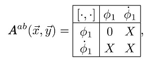 where ‘X' stands for generally non-vanishing entries. According to Dirac–Bergmann's terminology, both constraints are second class. As a result, the number of DOFs is given by
$\begin{eqnarray}{\#}_{{\rm{DOF}}}=\frac{2\times {4}_{{\rm{var}}}-1\times {2}_{2{\rm{nd}}}}{2}=3,\end{eqnarray}$
as expected.In the following, we will examine under which condition the number of DOFs can be less than 3, and in particular there are only 2 dynamical DOFs propagating. For the sake of simplicity, we focus on the case in which the coefficients in the Lagrangian (i.e. f3,1, f4,1 etc) are polynomials of A0 and $\bar{X}$.
4. The first degeneracy condition
As discussed in the previous section, in order to have number of DOFs less than 3, a necessary condition is that the Poisson bracket between φ1 and ${\dot{\phi }}_{1}$ must be vanishing (at least weakly). That is, we must require
$\begin{eqnarray}[{\phi }_{1}(\overrightarrow{x}),{\dot{\phi }}_{1}(\overrightarrow{y})]\approx 0,\end{eqnarray}$
which we refer to as the first degeneracy condition.After a lengthy but straightforward computation, the Poisson bracket can be written as
$\begin{eqnarray}\begin{array}{rcl}[{\phi }_{1}(\overrightarrow{x}),{\dot{\phi }}_{1}(\overrightarrow{y})] & = & {{ \mathcal F }}_{1}(\overrightarrow{x}){\delta }^{(3)}(\overrightarrow{y}-\overrightarrow{x})\\ & & +{{ \mathcal F }}^{i}(\overrightarrow{x})\frac{\partial }{\partial {y}^{i}}{\delta }^{(3)}(\overrightarrow{y}-\overrightarrow{x})\\ & & +{{ \mathcal F }}_{2}(\overrightarrow{x})\frac{{\partial }^{2}}{\partial {y}^{i}\partial {y}_{i}}{\delta }^{(3)}(\overrightarrow{y}-\overrightarrow{x}),\end{array}\end{eqnarray}$
where the coefficients are given by $\begin{eqnarray}\begin{array}{rcl}{{ \mathcal F }}_{1} & = & -\frac{\partial { \mathcal A }}{\partial {A}_{0}}{\partial }_{i}{{\rm{\Pi }}}^{i}-\frac{\partial { \mathcal B }}{\partial {A}_{0}}{({{\rm{\Pi }}}^{i})}^{2}\\ & & -\frac{\partial {{ \mathcal C }}_{i}^{(0,i)}}{\partial {A}_{0}}{{\rm{\Pi }}}^{i}-\frac{\partial {{ \mathcal D }}^{(0,i)}}{\partial {A}_{0}}\\ & & +\left(\frac{\partial {f}_{4,2}}{\partial {A}_{k}}{\partial }_{i}{A}^{i}+\frac{\partial {f}_{3,1}}{\partial {A}_{k}}\right)(2{ \mathcal B }{{\rm{\Pi }}}_{k}+{{ \mathcal C }}_{k}^{(0,i)}),\end{array}\end{eqnarray}$
$\begin{eqnarray}\begin{array}{rcl}{{ \mathcal F }}^{i} & = & \left[\frac{\partial }{\partial {A}_{0}}\left(\frac{{h}_{4,3}}{2{h}_{4,1}}\right)+\frac{\partial }{\partial {A}_{0}}\left(\frac{{h}_{4,3}}{2{h}_{4,1}}\right)\right.\\ & & \left.-2\frac{\partial {f}_{4,2}}{\partial {A}_{0}}{ \mathcal K }+2{f}_{4,2}\frac{\partial { \mathcal K }}{\partial {A}_{0}}\right]{{\rm{\Pi }}}^{i}\\ & & +6\frac{\partial }{\partial {A}_{0}}\left({h}_{4,2}-\frac{{({h}_{4,3})}^{2}}{4{h}_{4,1}}\right){\partial }^{i}{A}_{0}\\ & & +\frac{\partial {f}_{4,2}}{\partial {A}_{0}}{{ \mathcal W }}^{i(0)}+{f}_{4,2}\frac{\partial {{ \mathcal W }}^{i(0)}}{\partial {A}_{0}}\\ & & +\left(\frac{\partial {f}_{4,2}}{\partial {A}_{i}}{\partial }_{l}{A}^{l}+\frac{\partial {f}_{3,1}}{\partial {A}_{i}}\right){ \mathcal A }\\ & & +(2{ \mathcal B }{{\rm{\Pi }}}^{i}+{{ \mathcal C }}^{i(0,i)}){f}_{4,2}\\ & & +\left[\frac{\partial }{\partial {A}_{0}}({f}_{4,2}{ \mathcal A }){\partial }^{i}{A}_{0}+\frac{\partial }{\partial {A}_{k}}({f}_{4,2}{ \mathcal A }){\partial }^{i}{A}_{k}\right],\end{array}\end{eqnarray}$
and $\begin{eqnarray}{{ \mathcal F }}_{2}={f}_{4,2}{ \mathcal A }+2{h}_{4,2}-\frac{{({h}_{4,3})}^{2}}{2{h}_{4,1}}.\end{eqnarray}$
In deriving these expressions, we have used integrations by parts. For example, we have $\begin{eqnarray}\begin{array}{l}\displaystyle \int {{\rm{d}}}^{3}z\,{f}_{4,2}{ \mathcal A }{\partial }_{{x}^{i}}{\delta }^{(3)}(\overrightarrow{x}-\overrightarrow{z}){\partial }^{{y}^{i}}{\delta }^{(3)}(\overrightarrow{y}-\overrightarrow{z})\\ =-{f}_{4,2}{ \mathcal A }{\partial }_{{x}^{i}}{\partial }^{{x}^{i}}{\delta }^{(3)}(\overrightarrow{y}-\overrightarrow{x})\\ \quad -\,\left[\frac{\partial }{\partial {A}_{0}}({f}_{4,2}{ \mathcal A }){\partial }_{{x}^{i}}{A}_{0}+\frac{\partial }{\partial {A}_{k}}({f}_{4,2}{ \mathcal A }){\partial }_{{x}^{i}}{A}_{k}\right]\\ \quad \times \,{\partial }^{{x}^{i}}{\delta }^{(3)}(\overrightarrow{y}-\overrightarrow{x}).\end{array}\end{eqnarray}$
In order to have a vanishing Poisson bracket (4.1 ), we must require that 4.7 ) is satisfied if and only if all the three coefficients are vanishing separately, i.e.
$\begin{eqnarray}\begin{array}{l}{{ \mathcal F }}_{1}(\overrightarrow{x}){\delta }^{(3)}(\overrightarrow{y}-\overrightarrow{x})+{{ \mathcal F }}^{i}(\overrightarrow{x})\frac{\partial {\delta }^{(3)}(\overrightarrow{y}-\overrightarrow{x})}{\partial {y}^{i}}\\ +\,{{ \mathcal F }}_{2}(\overrightarrow{x})\frac{{\partial }^{2}{\delta }^{(3)}(\overrightarrow{y}-\overrightarrow{x})}{\partial {y}^{i}\partial {y}_{i}}=0.\end{array}\end{eqnarray}$
Note we have used ‘strong' equality here. The reason is that it is not possible for $[{\phi }_{1},{\dot{\phi }}_{1}]$ to be a linear combination of φ1 and ${\dot{\phi }}_{1}$, since the orders of spatial derivatives of ${{ \mathcal F }}_{1}$, ${\partial }_{i}{{ \mathcal F }}^{i}$ and ${\partial }^{2}{{ \mathcal F }}_{2}$ are different. This can be seen more explicitly by evaluating the Poisson bracket $[{\phi }_{1}(\overrightarrow{x}),{\dot{\phi }}_{1}(\overrightarrow{y})]$ with arbitrary test functions $A(\overrightarrow{x})$ and $B(\overrightarrow{y})$, which yields $\begin{eqnarray*}\begin{array}{rcl}0 & = & \displaystyle \int {{\rm{d}}}^{3}x{{\rm{d}}}^{3}yA(\overrightarrow{x})B(\overrightarrow{y})[{\phi }_{1}(\overrightarrow{x}),{\dot{\phi }}_{1}(\overrightarrow{y})]\\ & \simeq & \displaystyle \int {{\rm{d}}}^{3}x{{\rm{d}}}^{3}y\left(\Space{0ex}{3.5ex}{0ex}A(\overrightarrow{x})B(\overrightarrow{y}){{ \mathcal F }}_{1}(\overrightarrow{x})\right.\\ & & -A(\overrightarrow{x})\frac{\partial B(\overrightarrow{y})}{\partial {y}^{i}}{{ \mathcal F }}^{i}(\overrightarrow{x})\\ & & \left.+A(\overrightarrow{x})\frac{{\partial }^{2}B(\overrightarrow{y})}{\partial {y}^{i}\partial {y}_{i}}{{ \mathcal F }}_{2}(\overrightarrow{x})\right){\delta }^{(3)}(y-\overrightarrow{x})\\ & = & \displaystyle \int {{\rm{d}}}^{3}x\left(\Space{0ex}{3.5ex}{0ex}A(\overrightarrow{x})B(\overrightarrow{x}){{ \mathcal F }}_{1}(\overrightarrow{x})\right.\\ & & \left.-A(\overrightarrow{x})\frac{\partial B(\overrightarrow{x})}{\partial {x}^{i}}{{ \mathcal F }}^{i}(\overrightarrow{x})+A(\overrightarrow{x})\frac{{\partial }^{2}B(\overrightarrow{x})}{\partial {x}^{i}\partial {x}_{i}}{{ \mathcal F }}_{2}(\overrightarrow{x})\right).\end{array}\end{eqnarray*}$
Due to the arbitrariness of the test functions, equation ( $\begin{eqnarray}{{ \mathcal F }}_{1}=0,\,{{ \mathcal F }}^{i}=0,\,{{ \mathcal F }}_{2}=0.\end{eqnarray}$
Essentially, this is because they involve terms of differential orders in spatial derivatives.Equation (4.8 ) are 3 differential equations for the coefficients, which then constitute the explicit form of the first degeneracy condition. After plugging (3.3 ), i.e. Πi = 2h4,1∂0Ai + h4,3∂iA0, we can solve
$\begin{eqnarray}{f}_{4,2}={C}_{1}{A}_{0}+{C}_{2},\,{h}_{4,1}=\frac{1}{{C}_{1}{A}_{0}+{C}_{2}},\end{eqnarray}$
where C1 and C2 are constants. As we have mentioned before, in this work we focus on the case in which the coefficients are polynomials of A0 and $\bar{X}$. This ansatz is adopted to make the solution space of the (functional) degeneracy conditions explicitly classifiable and to exhibit closed-form families of 2 DOF Lagrangians. The degeneracy conditions themselves can be formulated for more general coefficient functions (e.g. analytic functions admitting local series expansions around backgrounds), and the Hamiltonian/constraint logic below does not rely on polynomiality except when solving the conditions explicitly. With this assumption, there is no other possibility than that h4,1 is a constant. In other words, we must choose C1 = 0 in the above solutions.With this result, the Lagrangians satisfying the first degeneracy condition can be specified explicitly. For ${{ \mathcal L }}_{2}={f}_{2}({A}_{0},\bar{X})$, we find it must be linear in A0. That is, we may write
$\begin{eqnarray}{{ \mathcal L }}_{2}={f}_{2}\equiv {\bar{f}}_{2}(\bar{X})+{A}_{0}{\tilde{f}}_{2}(\bar{X}),\end{eqnarray}$
where ${\bar{f}}_{2}$ and ${\tilde{f}}_{2}$ are general polynomials of $\bar{X}$. For ${{ \mathcal L }}_{3}$, we find that f3,1 cannot depend on $\bar{X}$ but can be a general polynomial of A0, whereas f3,2 must be linear in A0. Thus we can write $\begin{eqnarray}\begin{array}{rcl}{{ \mathcal L }}_{3} & = & {f}_{3,1}({A}_{0}){\dot{A}}_{0}+{f}_{3,2}({A}_{0},\bar{X}){\partial }_{i}{A}^{i}\\ & \simeq & \left({\bar{f}}_{3,2}+{A}_{0}{\tilde{f}}_{3,2}\right){\partial }_{i}{A}^{i},\end{array}\end{eqnarray}$
where ${\bar{f}}_{3,2}$ and ${\tilde{f}}_{3,2}$ are general polynomials of $\bar{X}$. Note ${\dot{A}}_{0}$ term in ${{ \mathcal L }}_{3}$ is removed by integration by parts. For ${{ \mathcal L }}_{4}$, we find that h4,1, h4,2, h4,3 and f4,2 must be constants satisfying $\begin{eqnarray}{f}_{4,2}({f}_{4,2}+{h}_{4,3})=4\left({h}_{4,2}{h}_{4,1}-\frac{{({h}_{4,3})}^{2}}{4}\right).\end{eqnarray}$
Thus we may denote $\begin{eqnarray}\begin{array}{rc}{h}_{4,1} & =\alpha ,\,{f}_{4,2}=\beta ,\,{h}_{4,3}=\gamma ,\end{array}\end{eqnarray}$
$\begin{eqnarray}\begin{array}{r}{h}_{4,2}=\frac{{(\beta +\gamma )}^{2}-\beta \gamma }{4\alpha }.\end{array}\end{eqnarray}$
We also find that f4,3, f4,4 and f4,5 are linear in A0, yielding $\begin{eqnarray}\begin{array}{r}\begin{array}{l}{{ \mathcal L }}_{4}\simeq \left(\beta +\gamma \right){\dot{A}}_{i}{\partial }^{i}{A}_{0}\\ +\,\alpha {\dot{A}}_{i}{\dot{A}}^{i}+\frac{{(\beta +\gamma )}^{2}-\beta \gamma }{4\alpha }{\partial }_{i}{A}_{0}{\partial }^{i}{A}_{0}\\ +\,\left({\bar{f}}_{4,3}+{A}_{0}{\tilde{f}}_{4,3}\right){({\partial }_{i}{A}^{i})}^{2}\\ +\,\left({\bar{f}}_{4,4}+{A}_{0}{\tilde{f}}_{4,4}\right){\partial }_{i}{A}_{j}{\partial }^{i}{A}^{j}\\ +\,\left({\bar{f}}_{4,5}+{A}_{0}{\tilde{f}}_{4,5}\right){\partial }_{i}{A}_{j}{\partial }^{j}{A}^{i},\end{array}\end{array}\end{eqnarray}$
where ${\bar{f}}_{4,3}$, ${\tilde{f}}_{4,3}$, ${\bar{f}}_{4,4}$, ${\tilde{f}}_{4,4}$, ${\bar{f}}_{4,5}$ and ${\tilde{f}}_{4,5}$ are general polynomials of $\bar{X}$.When the first degeneracy condition is satisfied, i.e. $[{\phi }_{1},{\dot{\phi }}_{1}]\approx 0$, we have 4.10 ), (4.11 ) and (4.15 ). As a result, we can rewrite $\dot{\phi }$ as $\dot{\phi }={ \mathcal A }{\partial }_{i}{{\rm{\Pi }}}^{i}+{{ \mathcal D }}^{(0,i)}$.
$\begin{eqnarray}{ \mathcal A }=\frac{1}{2{c}_{4,1}}({f}_{4,2}-{h}_{4,3}),\,{ \mathcal B }=0,\,{{ \mathcal C }}_{i}^{(0,i)}=0,\end{eqnarray}$
and $\begin{eqnarray}\begin{array}{rcl}{{ \mathcal D }}^{(0,i)} & = & -\frac{\partial }{\partial {A}_{0}}[{f}_{2}+{f}_{3,2}{\partial }_{i}{A}^{i}\\ & & +{f}_{4,3}{({\partial }_{i}{A}^{i})}^{2}+{f}_{4,4}{\partial }_{i}{A}_{j}{\partial }^{i}{A}^{j}\\ & & +{f}_{4,5}{\partial }_{i}{A}_{j}{\partial }^{j}{A}^{i}],\end{array}\end{eqnarray}$
where the coefficients are given as in (In general, the next consistency condition ${\ddot{\phi }}_{1}\approx 0$ gives rise to a tertiary constraint, since the Poisson bracket $[{\dot{\phi }}_{1}(\overrightarrow{x}),{H}_{{\rm{C}}}]$ does not vanish weakly. The Dirac matrix now takes the schematic form 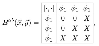 where again ‘X' denotes generally non-vanishing entries. If no additional constraints appear, (
4.18 ) implies that all three constraints $\{{\phi }_{1},{\dot{\phi }}_{1},{\ddot{\phi }}_{1}\}$ are second-class, leading formally to 2.5 DOFs. This can be understood as follows. For finite-dimensional systems, an odd-dimensional antisymmetric matrix has vanishing determinant and hence cannot be invertible (nondegenerate). However, this does not directly apply to ${B}_{ab}(\overrightarrow{x},\overrightarrow{y})$ in (4.18 ). In field theory, the object ${B}_{ab}(\overrightarrow{x},\overrightarrow{y})$ in (4.18 ) should be regarded as a differential operator acting on test functions, rather than a finite-dimensional matrix. Indeed, in field theories it is possible for an odd number of constraints (per spatial point) to be genuinely second-class when the Poisson brackets contain spatial derivatives of δ-functions and the corresponding operator is invertible after imposing appropriate boundary conditions. A classical example is the Floreanini–Jackiw chiral boson, which is commonly described as carrying one-half physical DOF [48] (see also [49]). Similar phenomena have also been discussed in Lorentz violating field theories, such as Hořava–Lifshitz gravity [50] and spatially covariant gravity theories [44, 51–53], where an additional condition is required in general to ensure that the would-be half mode is absent and only the desired propagating modes remain. With this understanding, (4.18 ) indicates that if ${B}_{ab}(\overrightarrow{x},\overrightarrow{y})$ is invertible as an operator on the space of test functions, then $\{{\phi }_{1},{\dot{\phi }}_{1},{\ddot{\phi }}_{1}\}$ are second-class and the theory exhibits a residual half DOF, so that the total number of DOFs is formally 2.5. Our goal is precisely to exclude this possibility and ensure that only the two transverse polarizations propagate.
To achieve this, the Dirac matrix Bab in (4.18 ) must be degenerate, i.e.4.19 ) as the second degeneracy condition. It can be shown that $\det {B}^{ab}$ is proportional to the Poisson brackets $[{\dot{\phi }}_{1},{\dot{\phi }}_{1}]$ and $[{\phi }_{1},{\ddot{\phi }}_{1}]$, while it has nothing to do with $[{\dot{\phi }}_{1},{\ddot{\phi }}_{1}]$ or $[{\ddot{\phi }}_{1},{\ddot{\phi }}_{1}]$. Hence the condition (4.19 ) can be realized with either of the following two choices: 4.20 ) or (4.21 ) is satisfied, we have $\det {B}^{ab}=0$. We refer to (4.20 ) and (4.21 ) as the two branches of the second degeneracy condition.
$\begin{eqnarray}\det {B}^{ab}(\overrightarrow{x},\overrightarrow{y})=0,\end{eqnarray}$
which means there exists a nontrivial null vector ${V}_{b}(\overrightarrow{y})$ such that $\int {{\rm{d}}}^{3}y\,{B}^{ab}(\overrightarrow{x},\overrightarrow{y}){V}_{b}(\overrightarrow{y})=0$. We therefore refer to ( $\begin{eqnarray}[{\dot{\phi }}_{1}(\overrightarrow{x}),{\dot{\phi }}_{1}(\overrightarrow{y})]\approx 0,\end{eqnarray}$
or $\begin{eqnarray}[{\phi }_{1}(\overrightarrow{x}),{\ddot{\phi }}_{1}(\overrightarrow{y})]\approx 0.\end{eqnarray}$
If either (In the following section, we explore the conditions on the Lagrangians under which either (4.20 ) or (4.21 ) is satisfied. In certain cases, both of them can be satisfied simultaneously. As we will see below, if one of the two branches of the second degeneracy condition is satisfied, the theory propagates exactly two dynamical DOFs.
5. The second degeneracy condition
In the previous section, we showed that to further eliminate the remaining half DOF, the second degeneracy condition (4.19 ) must be satisfied. As discussed, this requirement can be realized by either (4.20 ) or (4.21 ), which we refer to as branch 1 and branch 2 of the second degeneracy condition. These two branches correspond to distinct patterns of constraints and lead to different classes of theories, which we analyze separately below.
5.1. Branch 1
We first consider branch 1, corresponding to (4.20 ). By evaluating the Poisson bracket $[{\dot{\phi }}_{1},{\dot{\phi }}_{1}]$ explicitly, we obtain 5.4 ), which we will discuss below.
$\begin{eqnarray}\begin{array}{rcl}[{\dot{\phi }}_{1}(\overrightarrow{x}),{\dot{\phi }}_{1}(\overrightarrow{y})] & = & {{ \mathcal F }}^{* k}(\overrightarrow{x})\frac{\partial }{\partial {y}^{k}}{\delta }^{(3)}(\overrightarrow{y}-\overrightarrow{x})\\ & & +{{ \mathcal F }}^{* }(\overrightarrow{x})\frac{{\partial }^{2}}{\partial {y}^{k}\partial {y}_{k}}{\delta }^{(3)}(\overrightarrow{y}-\overrightarrow{x}),\end{array}\end{eqnarray}$
where $\begin{eqnarray}\begin{array}{r}{{ \mathcal F }}^{* k}=2{ \mathcal A }\left[\frac{\partial {{ \mathcal D }}^{(0,i)}}{\partial {A}_{k}}+\frac{\partial }{\partial {A}_{l}}\left(\frac{\partial {f}_{3,2}}{\partial {A}_{0}}\right){\partial }^{k}{A}_{l}\right.\\ +\left.2\frac{\partial }{\partial {A}_{l}}\left(\frac{\partial {f}_{4,4}}{\partial {A}_{0}}\right){\partial }^{i}{A}^{k}{\partial }_{i}{A}_{l}\right],\end{array}\end{eqnarray}$
and $\begin{eqnarray}{{ \mathcal F }}^{* }=2{ \mathcal A }\left[\frac{\partial {f}_{3,2}}{\partial {A}_{0}}+2\frac{\partial }{\partial {A}_{0}}\left({f}_{4,3}+{f}_{4,4}+{f}_{4,5}\right){\partial }_{i}{A}^{i}\right].\end{eqnarray}$
Again, with the technique of test functions and the fact that $[{\dot{\phi }}_{1},{\dot{\phi }}_{1}]$ cannot be expressed as a linear combination of φ1 and ${\dot{\phi }}_{1}$, the condition $[{\dot{\phi }}_{1}(\overrightarrow{x}),{\dot{\phi }}_{1}(\overrightarrow{y})]\approx 0$ is equivalent to requiring $\begin{eqnarray}{{ \mathcal F }}^{* k}=0,\,{{ \mathcal F }}^{* }=0.\end{eqnarray}$
Depending on whether ${ \mathcal A }=0$ or not, we have two cases of solutions to (5.1.1. Case 1
The simplest solution to (5.4 ) is
$\begin{eqnarray}{ \mathcal A }=0,\end{eqnarray}$
which implies $\begin{eqnarray}{f}_{4,2}=-{h}_{4,3}.\end{eqnarray}$
After some manipulations, we can determine the Lagrangians satisfying (5.5 ) or equivalently (5.6 ), together with the first degeneracy condition. For ${{ \mathcal L }}_{2}={f}_{2}({A}_{0},\bar{X})$, we find it must be linear in A0, i.e.
$\begin{eqnarray}{{ \mathcal L }}_{2}={\bar{f}}_{2}(\bar{X})+{A}_{0}{\tilde{f}}_{2}(\bar{X}),\end{eqnarray}$
where ${\bar{f}}_{2}$ and ${\tilde{f}}_{2}$ are general polynomials of $\bar{X}$. For ${{ \mathcal L }}_{3}$, we find that f3,1 cannot depend on $\bar{X}$ but can be a general polynomial of A0, and f3,2 is linear in A0. Thus we can write $\begin{eqnarray}\begin{array}{rcl}{{ \mathcal L }}_{3} & = & {f}_{3,1}{\dot{A}}_{0}+\left({\bar{f}}_{3,2}+{A}_{0}{\tilde{f}}_{3.2}\right)\\ & & \times {\partial }_{i}{A}^{i}\simeq \left({\bar{f}}_{3,2}+{A}_{0}{\tilde{f}}_{3.2}\right){\partial }_{i}{A}^{i},\end{array}\end{eqnarray}$
where ${\bar{f}}_{3,2}$ and ${\tilde{f}}_{3,2}$ are general polynomials of $\bar{X}$. In the above, we have used the fact that ${f}_{3,1}({A}_{0}){\dot{A}}_{0}$ can be reduced by integration by parts. For ${{ \mathcal L }}_{4}$, we find that h4,1, h4,2, h4,3 and f4,2 must be constants satisfying $\begin{eqnarray}-{h}_{4,3}={f}_{4,2}=2\sqrt{{h}_{4,2}{h}_{4,1}}.\end{eqnarray}$
Defining $\begin{eqnarray}{h}_{4,1}={\alpha }_{1},\,{f}_{4,2}=-{h}_{4,3}={\beta }_{1},\,{h}_{4,2}=\frac{{\beta }_{1}^{2}}{4{\alpha }_{1}},\end{eqnarray}$
and noting that f4,3, f4,4, and f4,5 are linear in A0, we finally obtain $\begin{eqnarray}\begin{array}{rcl}{{ \mathcal L }}_{4} & = & {\alpha }_{1}{\dot{A}}_{i}{\dot{A}}^{i}+\frac{{\beta }_{1}^{2}}{4{\alpha }_{1}}{\partial }_{i}{A}_{0}{\partial }^{i}{A}_{0}\\ & & +\left({\bar{f}}_{4,3}+{A}_{0}{\tilde{f}}_{4,3}\right){({\partial }_{i}{A}^{i})}^{2}\\ & & +\left({\bar{f}}_{4,4}+{A}_{0}{\tilde{f}}_{4,4}\right){\partial }_{i}{A}_{j}{\partial }^{i}{A}^{j}\\ & & +\left({\bar{f}}_{4,5}+{A}_{0}{\tilde{f}}_{4,5}\right){\partial }_{i}{A}_{j}{\partial }^{j}{A}^{i},\end{array}\end{eqnarray}$
where ${\bar{f}}_{4,3}$, ${\tilde{f}}_{4,3}$, ${\bar{f}}_{4,4}$, ${\tilde{f}}_{4,4}$, ${\bar{f}}_{4,5}$ and ${\tilde{f}}_{4,5}$ are general polynomials of $\bar{X}$.With the above solutions for the Lagrangians, the Dirac matrix takes the form 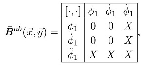 which is degenerate as $\det {\bar{B}}^{ab}(\overrightarrow{x},\overrightarrow{y})=0$. This implies the existence of one first-class constraint that can be expressed as a linear combination of the three constraints ${\phi }^{a}\,\equiv \{{\phi }_{1},{\dot{\phi }}_{1},{\ddot{\phi }}_{1}\}$. This can be seen from the fact that the degeneracy of Bab implies the existence of a null eigenvector
$\begin{eqnarray}\int {{\rm{d}}}^{3}y\,{\bar{B}}^{ab}(\overrightarrow{x},\overrightarrow{y}){{ \mathcal V }}_{b}(\overrightarrow{y})=0.\end{eqnarray}$
Using this null eigenvector, one can build a new constraint by combining the constraints $\begin{eqnarray}{\rm{\Phi }}=\int {{\rm{d}}}^{3}x\,{\phi }^{a}(\overrightarrow{x}){{ \mathcal V }}_{a}(\overrightarrow{x}),\end{eqnarray}$
which is clearly first-class as $\left[{\rm{\Phi }},{\phi }^{a}(\overrightarrow{x})\right]=0$.For our purposes, we do not need the explicit expression for the new first-class constraint. Instead, we formally denote it as ${\tilde{\phi }}_{1}$ and the rest two newly combined constraints as ${\tilde{\phi }}_{2}$ and ${\tilde{\phi }}_{3}$. Hence the new Dirac matrix becomes 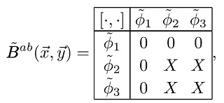 where ${\tilde{\phi }}_{a}$ are linear combinations of ${\phi }_{1},{\dot{\phi }}_{1},{\ddot{\phi }}_{1}$. Generally, the Poisson bracket $[{\phi }_{1}(\overrightarrow{x}),{\ddot{\phi }}_{1}(\overrightarrow{y})]$ does not vanish. Therefore the consistency condition for ${\ddot{\phi }}_{1}$ does not yield any further constraint. As a result, the theory possesses three constraints, of which one is first-class, two are second-class. For later convenience, we refer to theories in this case as ‘type-I' theories. The number of DOFs is counted as
$\begin{eqnarray}{\#}_{{\rm{dof}}}=\frac{2\times {4}_{{\rm{var}}}-2\times {1}_{1{\rm{st}}}-1\times {2}_{2{\rm{st}}}}{2}=2.\end{eqnarray}$
As we can see, the number of DOFs of the theory does reduce to two in this case.5.1.2. Case 2
Let us now focus on the other case, i.e. when ${ \mathcal A }\ne 0$. In this case, the second degeneracy condition (5.4 ) implies that quantities in the square brackets in (5.2 ) and (5.3 ) must be vanishing. This case seems more complicated, especially when explicitly substituting conjugate momenta results in higher order differential equations.
Nevertheless, after some manipulations, we can determine the Lagrangians satisfying both the first and the second degeneracy conditions in this case. For ${{ \mathcal L }}_{2}={f}_{2}(\bar{X})$, it must be linear in $\bar{X}$ and independent of A0. That is, we may write
$\begin{eqnarray}{{ \mathcal L }}_{2}={\bar{f}}_{2}\bar{X}+{\tilde{f}}_{2},\end{eqnarray}$
where ${\bar{f}}_{2}$ and ${\tilde{f}}_{2}$ are constants. For ${{ \mathcal L }}_{3}$, f3,1 is again independent of $\overline{X}$ but can generally depend on A0, while f3,2 is linear in $\overline{X}$. Thus we can write $\begin{eqnarray}\begin{array}{rcl}{{ \mathcal L }}_{3} & = & {f}_{3,1}{\dot{A}}_{0}+\left({\bar{f}}_{3,2}\overline{X}+{\tilde{f}}_{3.2}\right){\partial }_{i}{A}^{i}\\ & & \simeq \left({\bar{f}}_{3,2}\overline{X}+{\tilde{f}}_{3,2}\right){\partial }_{i}{A}^{i},\end{array}\end{eqnarray}$
where ${\bar{f}}_{3,2}$ and ${\tilde{f}}_{3,2}$ are constants and again we used integration by parts to suppress the term involving ${\dot{A}}_{0}$. For ${{ \mathcal L }}_{4}$, the coefficients h4,1, h4,2, h4,3 and f4,2 must be constants satisfying $\begin{eqnarray}{f}_{4,2}({f}_{4,2}+{h}_{4,3})=4\left({h}_{4,2}{h}_{4,1}-\frac{{({h}_{4,3})}^{2}}{4}\right),\end{eqnarray}$
which can be parametrized as $\begin{eqnarray}\begin{array}{r}{h}_{4,1}={\alpha }_{2},\,{f}_{4,2}={\beta }_{2},\,{h}_{4,3}={\gamma }_{2},\end{array}\end{eqnarray}$
$\begin{eqnarray}\begin{array}{r}{h}_{4,2}=\frac{{({\beta }_{2}+{\gamma }_{2})}^{2}-{\beta }_{2}{\gamma }_{2}}{4{\alpha }_{2}}.\end{array}\end{eqnarray}$
With f4,3, f4,4, and f4,5 linear in $\overline{X}$, the final form of ${{ \mathcal L }}_{4}$ is $\begin{eqnarray}\begin{array}{rcl}{{ \mathcal L }}_{4} & \simeq & \left({\beta }_{2}+{\gamma }_{2}\right){\dot{A}}_{i}{\partial }^{i}{A}_{0}+{\alpha }_{2}{\dot{A}}_{i}{\dot{A}}^{i}\\ & & +\frac{{({\beta }_{2}+{\gamma }_{2})}^{2}-{\beta }_{2}{\gamma }_{2}}{4{\alpha }_{2}}{\partial }_{i}{A}_{0}{\partial }^{i}{A}_{0}\\ & & +\left({\bar{f}}_{4,3}\overline{X}+{\tilde{f}}_{4,3}\right){({\partial }_{i}{A}^{i})}^{2}\\ & & +\left({\bar{f}}_{4,4}\overline{X}+{\tilde{f}}_{4,4}\right){\partial }_{i}{A}_{j}{\partial }^{i}{A}^{j}\\ & & +\left({\bar{f}}_{4,5}\overline{X}+{\tilde{f}}_{4,5}\right){\partial }_{i}{A}_{j}{\partial }^{j}{A}^{i},\end{array}\end{eqnarray}$
where ${\bar{f}}_{4,3}$, ${\tilde{f}}_{4,3}$, ${\bar{f}}_{4,4}$, ${\tilde{f}}_{4,4}$, ${\bar{f}}_{4,5}$ and ${\tilde{f}}_{4,5}$ are constants.The Poisson bracket $[{\phi }_{1}(\overrightarrow{x}),{\ddot{\phi }}_{1}(\overrightarrow{y})]$ vanishes automatically, yielding the Dirac matrix 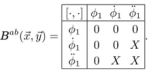 We find that the Poisson bracket $[{\ddot{\phi }}_{1}(\overrightarrow{x}),{H}_{{\rm{C}}}]$ is vanishing on the constraint surface, and
$\begin{eqnarray*}{\dddot{\phi }}_{1}\sim -\frac{{\beta }_{2}+{\gamma }_{2}}{{\alpha }_{2}}{\partial }^{3}({f}_{4,3}+{f}_{4,4}+{f}_{4,5})=0,\end{eqnarray*}$
which implies that there is no quaternary constraint. Then the number of DOF is counted as $\begin{eqnarray}{\#}_{{\rm{DOF}}}=\frac{2\times {4}_{{\rm{var}}}-2\times {1}_{1{\rm{st}}}-1\times {2}_{2{\rm{nd}}}}{2}=2.\end{eqnarray}$
Therefore, theories in this case is also of ‘type-I'.Interestingly, as we will see in section 5.2.1 , the case discussed here can be also viewed as a special solution in branch 2.
5.2. Branch 2
We now consider branch 2, corresponding to (4.21 ).
To proceed, we require the explicit expression for the tertiary constraint ${\ddot{\phi }}_{1}$, obtained from the consistency condition of ${\dot{\phi }}_{1}\approx 0$. Assuming that the Poisson bracket $[{\dot{\phi }}_{1}(\overrightarrow{x}),{H}_{{\rm{C}}}]$ does not vanish weakly, we find 3.7 ), ${{ \mathcal D }}^{(0,i)}$ given in (3.21 ), and 3.18 ), ${{ \mathcal W }}_{k}^{(0)}$ in (3.8 ), and ${{ \mathcal V }}^{(0,i)}$ in (3.9 ).
$\begin{eqnarray}{\ddot{\phi }}_{1}={{ \mathcal C }}_{k}^{* (0,i)}{{\rm{\Pi }}}^{k}+{{ \mathcal D }}^{* (0,i)},\end{eqnarray}$
where the coefficients ${{ \mathcal C }}^{* k(0,i)}$ and ${{ \mathcal D }}^{* (0,i)}$ contain no momenta and are given by $\begin{eqnarray}\begin{array}{rl}{{ \mathcal C }}^{* k(0,i)}= & \left[\frac{\partial {{ \mathcal D }}^{(0,i)}}{\partial {A}_{k}}+\frac{\partial }{\partial {A}_{l}}\left(\frac{\partial {f}_{3,2}}{\partial {A}_{0}}+2\frac{\partial {f}_{4,3}}{\partial {A}_{0}}{\partial }_{i}{A}^{i}\right){\partial }^{k}{A}_{l}\right.\\ & \left.+2\frac{\partial }{\partial {A}_{l}}\left(\frac{\partial {f}_{4,4}}{\partial {A}_{0}}{\partial }^{i}{A}^{k}+\frac{\partial {f}_{4,5}}{\partial {A}_{0}}{\partial }^{k}{A}^{i}\right){\partial }_{i}{A}_{l}\right]{ \mathcal K },\end{array}\end{eqnarray}$
with ${ \mathcal K }$ given in ( $\begin{eqnarray}\begin{array}{l}{{ \mathcal D }}^{* (0,i)}\\ =\left[\frac{\partial {{ \mathcal D }}^{(0,i)}}{\partial {A}_{k}}+\frac{\partial }{\partial {A}_{l}}\left(\frac{\partial {f}_{3,2}}{\partial {A}_{0}}+2\frac{\partial {f}_{4,3}}{\partial {A}_{0}}{\partial }_{i}{A}^{i}\right){\partial }^{k}{A}_{l}\right.\\ \quad \left.+2\frac{\partial }{\partial {A}_{l}}\left(\frac{\partial {f}_{4,4}}{\partial {A}_{0}}{\partial }^{i}{A}^{k}+\frac{\partial {f}_{4,5}}{\partial {A}_{0}}{\partial }^{k}{A}^{i}\right){\partial }_{i}{A}_{l}\right]{{ \mathcal W }}_{k}^{(0)}\\ \quad +\,{ \mathcal A }\left[\frac{{\partial }^{2}{{ \mathcal V }}^{(0,i)}}{\partial {A}_{0}\partial {A}_{k}}{\partial }_{k}{A}_{0}+{ \mathcal A }\frac{{\partial }^{2}{{ \mathcal V }}^{(0,i)}}{\partial {A}_{l}\partial {A}_{k}}{\partial }_{k}{A}_{l}\right.\\ \quad +\,\frac{\partial }{\partial {A}_{0}}\left(\frac{\partial {f}_{3,2}}{\partial {A}_{l}}\right){\partial }^{k}{A}_{l}{\partial }_{k}{A}_{0}+\frac{\partial }{\partial {A}_{m}}\\ \quad \times \,\left(\frac{\partial {f}_{3,2}}{\partial {A}_{0}}{\partial }^{k}{A}_{0}+\frac{\partial {f}_{3,2}}{\partial {A}_{l}}{\partial }^{k}{A}_{l}\right){\partial }_{k}{A}_{m}\\ \quad +\,\frac{\partial }{\partial {A}_{0}}\left(\frac{\partial {f}_{4,3}}{\partial {A}_{l}}\right){\partial }_{i}{A}^{i}{\partial }^{k}{A}_{l}{\partial }_{k}{A}_{0}+\frac{\partial }{\partial {A}_{m}}\\ \quad \times \,\left(\frac{\partial {f}_{4,3}}{\partial {A}_{0}}{\partial }_{i}{A}^{i}{\partial }^{k}{A}_{0}+\frac{\partial {f}_{4,3}}{\partial {A}_{l}}{\partial }_{i}{A}^{i}{\partial }^{k}{A}_{l}\right){\partial }_{k}{A}_{m}\\ \quad +\,\frac{\partial }{\partial {A}_{0}}\left(\frac{\partial {f}_{4,4}}{\partial {A}_{l}}\right){\partial }^{i}{A}^{k}{\partial }_{i}{A}_{l}{\partial }_{k}{A}_{0}\\ \quad +\,\frac{\partial }{\partial {A}_{m}}\left(\frac{\partial {f}_{4,4}}{\partial {A}_{0}}{\partial }^{i}{A}^{k}{\partial }_{i}{A}_{0}+\frac{\partial {f}_{4,4}}{\partial {A}_{l}}{\partial }^{i}{A}^{k}{\partial }_{i}{A}_{l}\right){\partial }_{k}{A}_{m}\\ \quad +\,\frac{\partial }{\partial {A}_{0}}\left(\frac{\partial {f}_{4,5}}{\partial {A}_{l}}\right){\partial }^{k}{A}^{i}{\partial }_{i}{A}_{l}{\partial }_{k}{A}_{0}\\ \quad +\,\left.\frac{\partial }{\partial {A}_{m}}\left(\frac{\partial {f}_{4,5}}{\partial {A}_{0}}{\partial }^{k}{A}^{i}{\partial }_{i}{A}_{0}+\frac{\partial {f}_{4,5}}{\partial {A}_{l}}{\partial }^{k}{A}^{i}{\partial }_{i}{A}_{l}\right){\partial }_{k}{A}_{m}\right],\end{array}\end{eqnarray}$
where ${ \mathcal A }$ is given in (After a tedious but straightforward calculation, we obtain the Poisson bracket 5.30 ) with the substitution of Πi = 2h4,1∂0Ai + h4,3∂iA0, we can get the conditions on the coefficients.
$\begin{eqnarray}\begin{array}{rcl}[{\phi }_{1}(\overrightarrow{x}),{\ddot{\phi }}_{1}(\overrightarrow{y})] & = & {\tilde{{ \mathcal F }}}^{k}\frac{\partial }{\partial {y}^{k}}{\delta }^{(3)}(\overrightarrow{y}-\overrightarrow{x})\\ & & +{\tilde{{ \mathcal F }}}_{1}{\delta }^{(3)}(\overrightarrow{y}-\overrightarrow{x}),\end{array}\end{eqnarray}$
where $\begin{eqnarray}\begin{array}{rcl}{\tilde{{ \mathcal F }}}_{1} & = & -\frac{\partial {{ \mathcal C }}^{* k(0,i)}}{\partial {A}_{0}}{{\rm{\Pi }}}_{k}-\frac{\partial {{ \mathcal D }}^{* (0,i)}}{\partial {A}_{0}}\\ & & -\frac{\partial {f}_{4,2}}{\partial {A}_{k}}{\partial }_{i}{A}^{i}{{ \mathcal C }}_{k}^{* (0,i)}-\frac{\partial {f}_{3,1}}{\partial {A}_{k}}{{ \mathcal C }}_{k}^{* (0,i)},\end{array}\end{eqnarray}$
and $\begin{eqnarray}\begin{array}{l}{\tilde{{ \mathcal F }}}^{k}\,=\,\left[\frac{\partial {{ \mathcal D }}^{(0,i)}}{\partial {A}_{k}}+\frac{\partial }{\partial {A}_{l}}\left(\frac{\partial {f}_{3,2}}{\partial {A}_{0}}+2\frac{\partial {f}_{4,3}}{\partial {A}_{0}}{\partial }_{i}{A}^{i}\right){\partial }^{k}{A}_{l}\right.\\ \left.+2\frac{\partial }{\partial {A}_{l}}\left(\frac{\partial {f}_{4,4}}{\partial {A}_{0}}{\partial }^{i}{A}^{k}+\frac{\partial {f}_{4,5}}{\partial {A}_{0}}{\partial }^{k}{A}^{i}\right){\partial }_{i}{A}_{l}\right]\\ \,\times \frac{{h}_{4,3}}{2{h}_{4,1}}-{f}_{4,2}{{ \mathcal C }}^{* k(0,i)}\\ \,+{ \mathcal A }\left[\frac{{\partial }^{2}{{ \mathcal V }}^{(0,i)}}{\partial {A}_{0}\partial {A}_{k}}+\frac{\partial }{\partial {A}_{0}}\left(\frac{\partial {f}_{3,2}}{\partial {A}_{l}}\right){\partial }^{k}{A}_{l}\right.\\ \,+\frac{\partial }{\partial {A}_{m}}\left(\frac{\partial {f}_{3,2}}{\partial {A}_{0}}\right){\partial }^{k}{A}_{m}\\ \,+\frac{\partial }{\partial {A}_{0}}\left(\frac{\partial {f}_{4,3}}{\partial {A}_{l}}\right){\partial }_{i}{A}^{i}{\partial }^{k}{A}_{l}\\ \,+\frac{\partial }{\partial {A}_{m}}\left(\frac{\partial {f}_{4,3}}{\partial {A}_{0}}\right){\partial }_{i}{A}^{i}{\partial }^{k}{A}_{m}\\ \,+\frac{\partial }{\partial {A}_{0}}\left(\frac{\partial {f}_{4,4}}{\partial {A}_{l}}\right){\partial }^{i}{A}^{k}{\partial }_{i}{A}_{l}\\ \,+\frac{\partial }{\partial {A}_{m}}\left(\frac{\partial {f}_{4,4}}{\partial {A}_{0}}\right){\partial }^{k}{A}^{i}{\partial }_{i}{A}_{m}\\ \,+\frac{\partial }{\partial {A}_{0}}\left(\frac{\partial {f}_{4,5}}{\partial {A}_{l}}\right){\partial }^{k}{A}^{i}{\partial }_{i}{A}_{l}\\ \,\left.+\frac{\partial }{\partial {A}_{m}}\left(\frac{\partial {f}_{4,5}}{\partial {A}_{0}}\right){\partial }^{i}{A}^{k}{\partial }_{i}{A}_{m}\right].\end{array}\end{eqnarray}$
Again, using the technique of test functions and noting that $[{\phi }_{1}(\overrightarrow{x}),{\ddot{\phi }}_{1}(\overrightarrow{y})]$ cannot be expressed as a linear combination of φ1, ${\dot{\phi }}_{1}$ and ${\ddot{\phi }}_{1}$, the condition $[{\phi }_{1}(\overrightarrow{x}),{\ddot{\phi }}_{1}(\overrightarrow{y})]\approx 0$ implies $\begin{eqnarray}{\tilde{{ \mathcal F }}}_{1}=0,\,{\tilde{{ \mathcal F }}}^{k}=0.\end{eqnarray}$
By solving (Solving (5.30 ), which consists of two differential equations for the coefficients, is generally difficult. Nevertheless, we can discuss two special cases by assuming that the coefficients depend either on A0 or $\overline{X}$ only, which simplifies the analysis. As we will see below, one case yields four second-class constraints, while the other case yields two first-class constraints.
5.2.1. Case 1
Let us focus on the first case, i.e.5.25 ) and (5.26 ) can be simplified to be
$\begin{eqnarray}\frac{\partial {f}_{2}}{\partial {A}_{0}}=0,\,\frac{\partial {f}_{m,n}}{\partial {A}_{0}}=0,\end{eqnarray}$
which implies that the coefficients depend on $\overline{X}$ only. Under this assumption, ${{ \mathcal C }}^{* k(0,i)}$ and ${{ \mathcal D }}^{* (0,i)}$ defined in ( $\begin{eqnarray}{{ \mathcal C }}^{* k(0,i)}=0,\end{eqnarray}$
and $\begin{eqnarray}\begin{array}{rcl}{{ \mathcal D }}^{* (0,i)} & = & { \mathcal A }\left(\frac{{\partial }^{2}{{ \mathcal V }}^{(0,i)}}{\partial {A}_{l}\partial {A}_{k}}{\partial }_{k}{A}_{l}+\frac{{\partial }^{2}{f}_{3,2}}{\partial {A}_{m}\partial {A}_{l}}{\partial }^{k}{A}_{l}{\partial }_{k}{A}_{m}\right.\\ & & +\frac{{\partial }^{2}{f}_{4,3}}{\partial {A}_{m}\partial {A}_{l}}{\partial }_{i}{A}^{i}{\partial }^{k}{A}_{l}{\partial }_{k}{A}_{m}\\ & & +\frac{{\partial }^{2}{f}_{4,4}}{\partial {A}_{m}\partial {A}_{l}}{\partial }^{i}{A}^{k}{\partial }_{i}{A}_{l}{\partial }_{k}{A}_{m}\\ & & +\left.\frac{{\partial }^{2}{f}_{4,5}}{\partial {A}_{m}\partial {A}_{l}}{\partial }^{k}{A}^{i}{\partial }_{i}{A}_{l}{\partial }_{k}{A}_{m}\right).\end{array}\end{eqnarray}$
In this case, the Dirac matrix takes the form 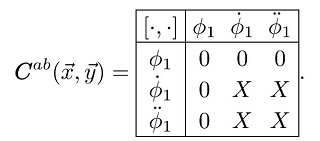 The consistency condition of ${\ddot{\phi }}_{1}$ yields
$\begin{eqnarray}\int {{\rm{d}}}^{3}y\,[{\phi }_{1}(\overrightarrow{x}),{\ddot{\phi }}_{1}(\overrightarrow{y})]\nu (\overrightarrow{y})\approx -[{\ddot{\phi }}_{1}(\overrightarrow{x}),{H}_{{\rm{C}}}].\end{eqnarray}$
Here $\nu (\overrightarrow{y})$ is the Lagrange multiplier associated with the primary constraint φ1 in the total Hamiltonian, which reads ${H}_{{\rm{T}}}={H}_{{\rm{C}}}+\int {{\rm{d}}}^{3}y\,\nu (\overrightarrow{y}){\phi }_{1}(\overrightarrow{y})$. We need to calculate the Poisson bracket $[{\ddot{\phi }}_{1}(\overrightarrow{x}),{H}_{{\rm{C}}}]$ with ${\ddot{\phi }}_{1}={{ \mathcal C }}_{k}^{* (0,i)}{{\rm{\Pi }}}^{k}+{{ \mathcal D }}^{* (0,i)}$. We find $\begin{eqnarray}\begin{array}{rc}[{\ddot{\phi }}_{1}(\overrightarrow{x}),{H}_{{\rm{C}}}] & ={{\rm{\Theta }}}_{m}^{(0,i)}{{\rm{\Pi }}}^{m}+{{\rm{\Delta }}}^{(0,i)},\end{array}\end{eqnarray}$
where $\begin{eqnarray*}\begin{array}{rcl}{{\rm{\Theta }}}^{m(0,i)} & = & { \mathcal A }{ \mathcal K }\left[\frac{1}{{ \mathcal A }}\frac{\partial {{ \mathcal D }}^{* (0,i)}}{\partial {A}_{m}}-{\partial }_{k}\left(\frac{{\partial }^{2}{{ \mathcal V }}^{(0,i)}}{\partial {A}_{m}\partial {A}_{k}}\right)\right.\\ & & +{\partial }^{m}\left(\frac{{\partial }^{2}{f}_{3,2}}{\partial {A}_{l}\partial {A}_{k}}\right){\partial }_{k}{A}_{l}\\ & & +2{\partial }^{m}\left(\frac{{\partial }^{2}{f}_{4,3}}{\partial {A}_{l}\partial {A}_{k}}\right){\partial }_{i}{A}^{i}{\partial }_{k}{A}_{l}\\ & & +2{\partial }_{i}\left(\frac{{\partial }^{2}{f}_{4,4}}{\partial {A}_{l}\partial {A}_{k}}\right){\partial }^{i}{A}^{m}{\partial }_{k}{A}_{l}\\ & & +2{\partial }^{m}\left(\frac{{\partial }^{2}{f}_{4,5}}{\partial {A}_{l}\partial {A}_{k}}\right){\partial }^{m}{A}^{i}{\partial }_{k}{A}_{l}\end{array}\end{eqnarray*}$
$\begin{eqnarray}\begin{array}{rcl} & & +{\partial }^{m}\left(\frac{{\partial }^{2}{f}_{4,3}}{\partial {A}_{i}\partial {A}_{l}}\right){\partial }^{k}{A}_{l}{\partial }_{k}{A}_{i}\\ & & +2{\partial }^{k}\left(\frac{{\partial }^{2}{f}_{4,3}}{\partial {A}_{l}\partial {A}_{m}}\right){\partial }_{i}{A}^{i}{\partial }_{k}{A}_{l}\\ & & +{\partial }^{i}\left(\frac{{\partial }^{2}{f}_{4,4}}{\partial {A}_{k}\partial {A}_{l}}\right){\partial }_{i}{A}_{l}{\partial }^{m}{A}_{k}\\ & & +{\partial }_{i}\left(\frac{{\partial }^{2}{f}_{4,4}}{\partial {A}_{l}\partial {A}_{m}}\right){\partial }^{i}{A}^{k}{\partial }_{k}{A}_{l}\\ & & +{\partial }_{k}\left(\frac{{\partial }^{2}{f}_{4,4}}{\partial {A}_{m}\partial {A}_{l}}\right){\partial }^{i}{A}^{k}{\partial }_{i}{A}_{l}\\ & & +{\partial }^{k}\left(\frac{{\partial }^{2}{f}_{4,5}}{\partial {A}_{i}\partial {A}_{l}}\right){\partial }^{m}{A}_{l}{\partial }_{k}{A}_{i}\\ & & +{\partial }_{i}\left(\frac{{\partial }^{2}{f}_{4,5}}{\partial {A}_{l}\partial {A}_{m}}\right){\partial }^{k}{A}^{i}{\partial }_{k}{A}_{l}\\ & & \left.+{\partial }_{k}\left(\frac{{\partial }^{2}{f}_{4,5}}{\partial {A}_{m}\partial {A}_{l}}\right){\partial }^{k}{A}^{i}{\partial }_{i}{A}_{l}\right],\end{array}\end{eqnarray}$
and $\begin{eqnarray}\begin{array}{rcl}{{\rm{\Delta }}}^{(0,i)} & = & { \mathcal A }{{ \mathcal W }}_{m}^{(0)}\left[\frac{1}{{ \mathcal A }}\frac{\partial {{ \mathcal D }}^{* (0,i)}}{\partial {A}_{m}}-{\partial }_{k}\left(\frac{{\partial }^{2}{{ \mathcal V }}^{(0,i)}}{\partial {A}_{m}\partial {A}_{k}}\right)\right.\\ & & +{\partial }^{m}\left(\frac{{\partial }^{2}{f}_{3,2}}{\partial {A}_{l}\partial {A}_{k}}\right){\partial }_{k}{A}_{l}\\ & & +2{\partial }^{m}\left(\frac{{\partial }^{2}{f}_{4,3}}{\partial {A}_{l}\partial {A}_{k}}\right){\partial }_{i}{A}^{i}{\partial }_{k}{A}_{l}\\ & & +2{\partial }_{i}\left(\frac{{\partial }^{2}{f}_{4,4}}{\partial {A}_{l}\partial {A}_{k}}\right){\partial }^{i}{A}^{m}{\partial }_{k}{A}_{l}\\ & & +2{\partial }^{m}\left(\frac{{\partial }^{2}{f}_{4,5}}{\partial {A}_{l}\partial {A}_{k}}\right){\partial }^{m}{A}^{i}{\partial }_{k}{A}_{l}\\ & & +{\partial }^{m}\left(\frac{{\partial }^{2}{f}_{4,3}}{\partial {A}_{i}\partial {A}_{l}}\right){\partial }^{k}{A}_{l}{\partial }_{k}{A}_{i}\\ & & +2{\partial }^{k}\left(\frac{{\partial }^{2}{f}_{4,3}}{\partial {A}_{l}\partial {A}_{m}}\right){\partial }_{i}{A}^{i}{\partial }_{k}{A}_{l}\\ & & +{\partial }^{i}\left(\frac{{\partial }^{2}{f}_{4,4}}{\partial {A}_{k}\partial {A}_{l}}\right){\partial }_{i}{A}_{l}{\partial }^{m}{A}_{k}\\ & & +{\partial }_{i}\left(\frac{{\partial }^{2}{f}_{4,4}}{\partial {A}_{l}\partial {A}_{m}}\right){\partial }^{i}{A}^{k}{\partial }_{k}{A}_{l}\\ & & +{\partial }_{k}\left(\frac{{\partial }^{2}{f}_{4,4}}{\partial {A}_{m}\partial {A}_{l}}\right){\partial }^{i}{A}^{k}{\partial }_{i}{A}_{l}\\ & & +{\partial }^{k}\left(\frac{{\partial }^{2}{f}_{4,5}}{\partial {A}_{i}\partial {A}_{l}}\right){\partial }^{m}{A}_{l}{\partial }_{k}{A}_{i}\\ & & +{\partial }_{i}\left(\frac{{\partial }^{2}{f}_{4,5}}{\partial {A}_{l}\partial {A}_{m}}\right){\partial }^{k}{A}^{i}{\partial }_{k}{A}_{l}\\ & & \left.+{\partial }_{k}\left(\frac{{\partial }^{2}{f}_{4,5}}{\partial {A}_{m}\partial {A}_{l}}\right){\partial }^{k}{A}^{i}{\partial }_{i}{A}_{l}\right].\end{array}\end{eqnarray}$
Note that the coefficients have been restricted by the condition $[{\phi }_{1},{\ddot{\phi }}_{1}]\approx 0$. In evaluating the spatial derivatives above, only spatial derivatives of Ai contribute. For example, $\begin{eqnarray*}{\partial }^{m}\left(\frac{{\partial }^{2}{f}_{3,2}}{\partial {A}_{l}\partial {A}_{k}}\right)=\frac{{\partial }^{3}{f}_{3,2}}{\partial {A}_{n}\partial {A}_{l}\partial {A}_{k}}{\partial }^{m}{A}_{n}.\end{eqnarray*}$
Depending on whether $[{\ddot{\phi }}_{1}(\overrightarrow{x}),{H}_{{\rm{C}}}]$ is vanishing weakly or not, we can further consider two sub-cases. In the special case where $[{\ddot{\phi }}_{1}(\overrightarrow{x}),{H}_{{\rm{C}}}]\approx 0$ on the constraint surface, no quaternary constraint arises. In this case, the Dirac matrix becomes 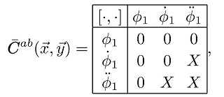 which indicates the emergence of a first-class constraint and thus the enhancement of the gauge symmetry. The resulting theory possesses one first-class constraint and two second-class constraints, and thus belongs to ‘type-I' theories. Comparing with the case in section
 5.1.2 , if the conditions discussed in section 5.1.2 are satisfied, the Poisson brackets $[{\phi }_{1},{\ddot{\phi }}_{1}]\approx 0$ and $[{\ddot{\phi }}_{1},{H}_{{\rm{C}}}]\approx 0$ will automatically be satisfied, but not vice versa. In other words, the case 2 of branch 1 discussed in section 5.1.2 is not independent in the sense that it can be viewed as the sub-case discussed here, i.e. as the special solution in case 1 of branch 2.
We then turn to the general case, where $[{\ddot{\phi }}_{1}(\overrightarrow{x}),{H}_{{\rm{C}}}]$ does not vanish weakly. This leads to a new quaternary constraint, yielding the Dirac matrix 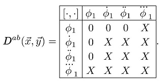 Generally, the Poisson bracket
$\begin{eqnarray}\begin{array}{rc}[{\phi }_{1}(\overrightarrow{x}),{\dddot{\phi }}_{1}(\overrightarrow{y})] & ={\tilde{{ \mathcal F }}}_{k}^{* }\frac{\partial }{\partial {y}_{k}}{\delta }^{(3)}(\overrightarrow{y}-\overrightarrow{x}),\end{array}\end{eqnarray}$
with $\begin{eqnarray}{\tilde{{ \mathcal F }}}_{k}^{* }=-{f}_{4,2}{{\rm{\Theta }}}_{k}^{(0,i)},\end{eqnarray}$
does not vanish weakly. Thus, in this case, the theory contains four second-class constraints, leading to the number of DOFs $\begin{eqnarray}{\#}_{{\rm{DOF}}}=\frac{2\times {4}_{{\rm{var}}}-1\times {4}_{2{\rm{nd}}}}{2}=2.\end{eqnarray}$
We refer to theories in this case as ‘type-II' theories. It is clear that this is a new situation different from the previous ones.In this case, we can determine the Lagrangians satisfying the second degeneracy condition. For ${{ \mathcal L }}_{2}={f}_{2}(\overline{X})$, we find that it must be nonlinear in $\overline{X}$. Hence, we may write
$\begin{eqnarray}{{ \mathcal L }}_{2}={f}_{2},\end{eqnarray}$
where f2 is a nonlinear polynomial of $\overline{X}$. For ${{ \mathcal L }}_{3}$, we find that f3,1 cannot depend on $\overline{X}$ but can be a general polynomial of A0, whereas f3,2 must be nonlinear in $\overline{X}$. Thus we can write $\begin{eqnarray}{{ \mathcal L }}_{3}={f}_{3,1}({A}_{0}){\dot{A}}_{0}+{\bar{f}}_{3,2}(\overline{X}){\partial }_{i}{A}^{i}\simeq {\bar{f}}_{3,2}(\overline{X}){\partial }_{i}{A}^{i},\end{eqnarray}$
where ${\bar{f}}_{3,2}$ is a nonlinear polynomial of $\overline{X}$. For ${{ \mathcal L }}_{4}$, we find that h4,1, h4,2, h4,3 and f4,2 must be constants satisfying $\begin{eqnarray}{f}_{4,2}({f}_{4,2}+{h}_{4,3})=4\left({h}_{4,2}{h}_{4,1}-\frac{{({h}_{4,3})}^{2}}{4}\right).\end{eqnarray}$
We therefore denote $\begin{eqnarray}\begin{array}{r}{h}_{4,1}={\alpha }_{2},\,{f}_{4,2}={\beta }_{2},\,{h}_{4,3}={\gamma }_{2},\end{array}\end{eqnarray}$
$\begin{eqnarray}\begin{array}{r}{h}_{4,2}=\frac{{({\beta }_{2}+{\gamma }_{2})}^{2}-{\beta }_{2}{\gamma }_{2}}{4{\alpha }_{2}}.\end{array}\end{eqnarray}$
We also find that f4,3, f4,4, and f4,5 are nonlinear in $\overline{X}$. Thus finally we have $\begin{eqnarray}\begin{array}{rcl}{{ \mathcal L }}_{4} & \simeq & \left({\beta }_{2}+{\gamma }_{2}\right){\dot{A}}_{i}{\partial }^{i}{A}_{0}+{\alpha }_{2}{\dot{A}}_{i}{\dot{A}}^{i}\\ & & +\frac{{({\beta }_{2}+{\gamma }_{2})}^{2}-{\beta }_{2}{\gamma }_{2}}{4{\alpha }_{2}}{\partial }_{i}{A}_{0}{\partial }^{i}{A}_{0}\\ & & +{f}_{4,3}{\left({\partial }_{i}{A}^{i}\right)}^{2}+{f}_{4,4}{\partial }_{i}{A}_{j}{\partial }^{i}{A}^{j}\\ & & +{f}_{4,5}{\partial }_{i}{A}_{j}{\partial }^{j}{A}^{i},\end{array}\end{eqnarray}$
where f4,3, f4,4, and f4,5 are nonlinear polynomials of $\overline{X}$.5.2.2. Case 2
Now let us turn to the other choice, given by
$\begin{eqnarray}\frac{\partial {f}_{2}}{\partial {A}_{k}}=0,\ \frac{\partial {f}_{m,n}}{\partial {A}_{k}}=0,\end{eqnarray}$
which indicates that all the coefficients depend only on A0. In this case, ${{ \mathcal C }}^{* k(0,i)}$ and ${{ \mathcal D }}^{* (0,i)}$ are greatly simplified as $\begin{eqnarray}{{ \mathcal C }}^{* k(0,i)}=0,\,{{ \mathcal D }}^{* (0,i)}=0.\end{eqnarray}$
Recalling that ${\dot{\phi }}_{1}={ \mathcal A }{\partial }_{i}{{\rm{\Pi }}}^{i}+{ \mathcal B }{({{\rm{\Pi }}}^{i})}^{2}+{{ \mathcal C }}_{i}^{(0,i)}{{\rm{\Pi }}}^{i}+{{ \mathcal D }}^{(0,i)}$ and $[{\dot{\phi }}_{1}(\overrightarrow{x}),{H}_{{\rm{C}}}]={{ \mathcal C }}_{k}^{* (0,i)}{{\rm{\Pi }}}^{k}+{{ \mathcal D }}^{* (0,i)}$, (5.51 ) implies that ${\ddot{\phi }}_{1}={{ \mathcal C }}_{k}^{* (0,i)}{{\rm{\Pi }}}^{k}+{{ \mathcal D }}^{* (0,i)}$ vanishes identically. Consequently, no additional constraints arise, and the Dirac matrix takes the form 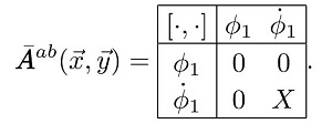 On the other hand, if $[{\dot{\phi }}_{1}(\overrightarrow{x}),{\dot{\phi }}_{1}(\overrightarrow{y})]$ given in (
5.1 ) does not vanish weakly, the number of DOFs is still 2.5 instead of 2. Therefore, we must further require that $[{\dot{\phi }}_{1}(\overrightarrow{x}),{\dot{\phi }}_{1}(\overrightarrow{y})]\approx 0$, which implies that 5.50 ), this result indicates that the coefficients fm,n must be constants.
$\begin{eqnarray*}\frac{\partial {f}_{m,n}}{\partial {A}_{0}}=0.\end{eqnarray*}$
Together with the assumption (Finally, the Dirac matrix becomes 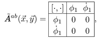 which indicates that the theory possesses two first-class constraints, with the number of DOFs given by
 Appendix for a brief reminder of the Hamiltonian formalism for Maxwell theory. However, due to the breaking of Lorentz invariance, the Lagrangians can be different from that of the Maxwell theory.
$\begin{eqnarray}{\#}_{{\rm{DOF}}}=\frac{2\times {4}_{{\rm{var}}}-2\times {2}_{1{\rm{st}}}}{2}=2.\end{eqnarray}$
We refer to theories in this case as ‘type-III' theories. The constraint structure in this case coincides exactly with that of the standard Maxwell theory. We refer to At this point, it is interesting to check the gauge transformation generated by the two first-class constraints φ1 and ${\dot{\phi }}_{1}$. Since all coefficients are constants in this case, ${\dot{\phi }}_{1}$ reduces to a Gauss-type constraint ${\dot{\phi }}_{1}={ \mathcal A }{\partial }_{i}{{\rm{\Pi }}}^{i}\approx $ with constant ${ \mathcal A }$. A convenient choice of the generator of gauge transformation is
$\begin{eqnarray*}\begin{array}{rcl}G[\epsilon ] & = & \displaystyle \int {{\rm{d}}}^{3}x\left(\Space{0ex}{3ex}{0ex}-\dot{\epsilon }(\overrightarrow{x}){\phi }_{1}(\overrightarrow{x})\right.\\ & & \left.+\frac{1}{{ \mathcal A }}\epsilon (\overrightarrow{x}){\dot{\phi }}_{1}(\overrightarrow{x})\right),\end{array}\end{eqnarray*}$
where $\epsilon (\overrightarrow{x})$ is the infinitesimal parameter. The transformations are thus given by $\begin{eqnarray*}\begin{array}{rcl}\delta {A}_{0}(\overrightarrow{x}) & = & \left[{A}_{0}(\overrightarrow{x}),G[\epsilon ]\right]=-\dot{\epsilon }(\overrightarrow{x}),\\ \delta {A}_{i}(\overrightarrow{x}) & = & \left[{A}_{i}(\overrightarrow{x}),G[\epsilon ]\right]={\partial }_{i}\epsilon (\overrightarrow{x}).\end{array}\end{eqnarray*}$
This makes explicit the close analogy to electromagnetism, where the Gauss-type constraint generates δAi = ∂iε.After some manipulations, we can determine the Lagrangians satisfying the second degeneracy condition. For ${{ \mathcal L }}_{2}={f}_{2}$, we find it must be a constant, namely,
$\begin{eqnarray}{{ \mathcal L }}_{2}={c}_{2},\end{eqnarray}$
which is thus trivial. For ${{ \mathcal L }}_{3}$, both f3,1 and f3,2 are constants, allowing us to write $\begin{eqnarray}{{ \mathcal L }}_{3}={c}_{3,1}{\dot{A}}_{0}+{c}_{3,2}{\partial }_{i}{A}^{i}\simeq 0,\end{eqnarray}$
where we denote f3,1 = c3,1 and f3,2 = c3,2. Clearly ${{ \mathcal L }}_{3}$ is also trivial since it is a sum of total derivatives. The only nontrivial Lagrangian is ${{ \mathcal L }}_{4}$. We find that h4,1, h4,2, h4,3 and f4,2 must be constants satisfying $\begin{eqnarray}{f}_{4,2}({f}_{4,2}+{h}_{4,3})=4\left({h}_{4,2}{h}_{4,1}-\frac{{({h}_{4,3})}^{2}}{4}\right).\end{eqnarray}$
We may denote $\begin{eqnarray}\begin{array}{rc}{h}_{4,1} & ={\alpha }_{3},\,{f}_{4,2}={\beta }_{3},\,{h}_{4,3}={\gamma }_{3},\end{array}\end{eqnarray}$
$\begin{eqnarray}\begin{array}{rc}{h}_{4,2} & =\frac{{({\beta }_{3}+{\gamma }_{3})}^{2}-{\beta }_{3}{\gamma }_{3}}{4{\alpha }_{3}}.\end{array}\end{eqnarray}$
We also find that f4,3, f4,4, and f4,5 are constants. Finally, we obtain $\begin{eqnarray}\begin{array}{rcl}{{ \mathcal L }}_{4} & \simeq & \left({\beta }_{3}+{\gamma }_{3}\right){\dot{A}}_{i}{\partial }^{i}{A}_{0}+{\alpha }_{3}{\dot{A}}_{i}{\dot{A}}^{i}\\ & & +\frac{{({\beta }_{3}+{\gamma }_{3})}^{2}-{\beta }_{3}{\gamma }_{3}}{4{\alpha }_{3}}{\partial }_{i}{A}_{0}{\partial }^{i}{A}_{0}\\ & & +\left({c}_{4,3}+{c}_{4,5}\right){\partial }_{i}{A}_{j}{\partial }^{j}{A}^{i}+{c}_{4,4}{\partial }_{i}{A}_{j}{\partial }^{i}{A}^{j},\end{array}\end{eqnarray}$
where we denote f4,3 = c4,3, f4,4 = c4,4 and f4,5 = c4,5.As a special case, when the system restores Lorentz invariance, the Lagrangian ${{ \mathcal L }}_{4}$ reduces to
$\begin{eqnarray*}\begin{array}{l}{{ \mathcal L }}_{4}\propto {\dot{A}}_{i}{\dot{A}}^{i}-{\partial }_{i}{A}_{j}{\partial }^{i}{A}^{j}+{\partial }_{i}{A}_{j}{\partial }^{j}{A}^{i}\\ +\,{\partial }_{i}{A}_{0}{\partial }^{i}{A}_{0}-2{\dot{A}}_{i}{\partial }^{i}{A}_{0},\end{array}\end{eqnarray*}$
which is nothing but the Maxwell theory.6. Conclusion
Recently, there has been growing interest in applying vector fields to cosmological and gravitational-wave model building. In general, breaking Lorentz symmetry and U(1) gauge invariance introduces an additional longitudinal mode, in addition to the two usual transverse modes of the vector field. In this work, we explored a class of spatially covariant vector field theories and investigated the conditions required to eliminate this extra DOF so that only two modes propagate.
In section 2 , we introduced the spatially covariant vector field theory. As a first attempt to construct a vector field theory with two DOFs, we turned off the effects of gravity and focused on a flat background. We assumed that the Lagrangians are polynomials built from the first derivatives of the vector field. We then performed a Hamiltonian analysis in section 3 , demonstrating that the theory generally propagates three DOFs unless specific conditions are imposed on the structure of the Lagrangian.
We found that the complete removal of the unwanted mode requires two degeneracy conditions. The first condition is derived in section 4 and given in (4.1 ), which identifies the Lagrangians in (4.10 ), (4.11 ) and (4.15 ). If only the first degeneracy condition is satisfied, the kernel ${B}_{ab}(\overrightarrow{x},\overrightarrow{y})$ defined in (4.18 ) is invertible, which means all three constraints $\{{\phi }_{1},{\dot{\phi }}_{1},{\ddot{\phi }}_{1}\}$ are second-class. As a result, the theory typically propagates 2.5 DOFs which is allowed in Lorentz-violating field theories. To fully eliminate the residual half DOF, the second degeneracy condition is necessary. This is given by (4.19 ), where the Dirac matrix Bab is defined in (4.18 ). There are two branches of solutions to (4.19 ), denoted as the first and second branches, expressed respectively in (4.20 ) and (4.21 ).
In section 5 , we analyzed both branches in detail, identifying three distinct types of consistent theories. For the first branch, we found two cases of solutions in section 5.1 . The corresponding Lagrangians are given in (5.7 ), (5.8 ) and (5.11 ) for the first case, and in (5.16 ), (5.17 ) and (5.21 ) for the second case. In both cases, the theories possess one first-class and two second-class constraints, which we refer to as ‘type-I' theories. For the second branch discussed in section 5.2 , we identified two special cases and thus two types of theories. The ‘type-II' theory has four second-class constraints, with nontrivial Lagrangians given in (5.45 ) and (5.49 ). The ‘type-III' theory admits two first-class constraints, and the only nontrivial Lagrangian is ${{ \mathcal L }}_{4}$ given in (5.60 ). Interestingly, the type-III theory encompasses the Maxwell theory as a special limit when Lorentz invariance is restored.
Our results show the possibility of constructing spatially covariant vector field theories that propagate only two DOFs, providing a foundation for future developments in Lorentz-violating field theories and their potential cosmological applications. In this work, we considered only first-order derivatives of the vector field and focused on a flat background. It will be interesting to extend the analysis by including higher-order derivatives of the vector field and incorporating the effects of gravity. Moreover, a systematic extension to curved backgrounds can be carried out by promoting the building blocks to a general foliated spacetime and replacing partial derivatives by spatially covariant derivatives. We will explore these issues in future work.
Appendix Hamiltonian formalism for Maxwell theory
Let us review the Hamiltonian formalism for Maxwell theory
$\begin{eqnarray*}{ \mathcal L }=-\frac{1}{4}{F}_{\mu \nu }{F}^{\mu \nu },\end{eqnarray*}$
where Fμν = 2∂[μAν].The momenta conjugate to Ai are ${{\rm{\Pi }}}^{i}={\dot{A}}^{i}-{\partial }^{i}{A}_{0}$. The absence of a kinetic term for the temporal component ${\dot{A}}_{0}$ leads to the primary constraint
$\begin{eqnarray*}{C}_{1}\equiv {{\rm{\Pi }}}^{0}\approx 0.\end{eqnarray*}$
The total Hamiltonian is $\begin{eqnarray*}{H}_{{\rm{T}}}=\int {{\rm{d}}}^{3}x({{ \mathcal H }}_{{\rm{C}}}+\lambda {C}_{1}),\end{eqnarray*}$
where $\begin{eqnarray*}{{ \mathcal H }}_{{\rm{C}}}=\frac{1}{2}{{\rm{\Pi }}}^{i}{{\rm{\Pi }}}_{i}+\frac{1}{2}{F}_{ij}{F}^{ij}-{A}_{0}{\partial }_{i}{{\rm{\Pi }}}^{i},\end{eqnarray*}$
and λ is an undetermined Lagrange multiplier.The consistency condition for ${\dot{C}}_{1}\approx 0$ gives
$\begin{eqnarray*}{\dot{C}}_{1}(\overrightarrow{x})=[{{\rm{\Pi }}}^{0}(\overrightarrow{x}),{H}_{C}]={\partial }_{i}{{\rm{\Pi }}}^{i}\equiv {C}_{2}(\overrightarrow{x})\approx 0,\end{eqnarray*}$
which yields the secondary constraint C2 ≈ 0. The consistency condition for C2 ≈ 0 is automatically satisfied, since $\begin{eqnarray*}{\dot{C}}_{2}(\overrightarrow{x})=\left[\frac{\partial {{\rm{\Pi }}}^{i}(\overrightarrow{x})}{\partial {x}^{i}},{H}_{{\rm{C}}}\right]=0.\end{eqnarray*}$
Therefore C1 ≈ 0 and C2 ≈ 0 are all the constraints in Maxwell theory.It is straightforward to calculate the Poisson brackets among these constraints, yielding the Dirac matrix for Maxwell theory: 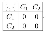 Thus, both constraints are first-class. The number of DOFs is thus given by
$\begin{eqnarray}{\#}_{{\rm{DOF}}}=\frac{2\times {4}_{{\rm{var}}}-2\times {2}_{1{\rm{st}}}}{2}=2,\end{eqnarray}$
which corresponds to the two transverse polarization modes of the photon.