


1. Introduction
2. Magnetically charged de-Sitter black holes
(i) In the regime where ε ≥ 0, the spacetime structure permits only two horizons: the black hole event horizon and the cosmological horizon.
(ii) In the regime where ε < 0, the spacetime horizon structure undergoes significant transformations, see the right panels in figure 2(a). For ε = −1, representing weak coupling strength, three distinct horizons emerge: the Cauchy horizon r−, black hole event horizon rh, and a cosmological horizon rc. As the coupling intensifies to εc ≈ −292.357, the system reaches a critical phase where the inner horizons merge into a single extremal black hole horizon rh, while the cosmological horizon rc persists. In the strong coupling limit (ε = −1000), only the cosmological horizon remains (r = rc), creating a causally connected region (r < rc and B(r) > 0) that exposes the central singularity—a clear violation of cosmic censorship resulting from the dominant coupling effects.
(iii) The behavior of the metric function B(r) with varying cosmological constant Λ is illustrated in figure 3.
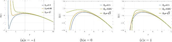
Figure 1. The metric function B(r) as a function of the radial coordinate r for different values of magnetic charge Qm with fixed M = 1 and Λ = 0.05. Panels (a)–(c) correspond to ε = −1, ε = 0, and ε = 1, respectively. The zeros of B(r) indicate horizons depending on parameters, there can be 0–3 horizons (cosmological horizon rc, event horizon rh, and possibly Cauchy horizon r−). |
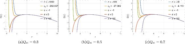
Figure 2. The metric function B(r) versus r for different values of the coupling parameter ε, with fixed M = 1 and Λ = 0.05. Panels (a)–(c) correspond to Qm = 0.3, Qm = 0.5, and Qm = 0.7, respectively. The zeros of B(r) indicate horizons depending on parameters, there can be 0–3 horizons (cosmological horizon rc, event horizon rh, and possibly Cauchy horizon r−). |
3. Wave equations and perturbations
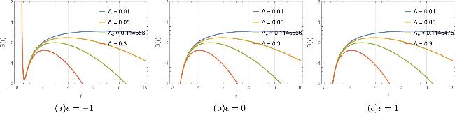
Figure 3. The metric function B(r) versus r for different values of the cosmological constant Λ, with fixed M = 1 and Qm = 0.3. Panels (a)–(c) correspond to ε = −1, ε = 0, and ε = 1, respectively. The zeros of B(r) indicate horizons depending on parameters, there can be 0–3 horizons (cosmological horizon rc, event horizon rh, and possibly Cauchy horizon r−). |
3.1. Scalar field perturbation
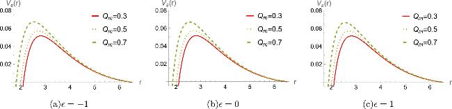
Figure 4. The effective potential Vs(r) for massless scalar field perturbation (l = 1) as a function of the radial coordinate r for different values of magnetic charge Qm. In all cases, we set M = 1 and Λ = 0.05. Panels (a)–(c) correspond to ε = −1, ε = 0, and ε = 1, respectively. As Qm decreases, the peak of the potential barrier shifts outward and its height is significantly suppressed. |
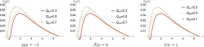
Figure 5. The effective potential Ve(r) for electromagnetic field perturbation (l = 1) as a function of the radial coordinate r for different values of magnetic charge Qm. In all cases, we set M = 1 and Λ = 0.05. Panels (a)–(c) correspond to ε = −1, ε = 0, and ε = 1, respectively. As Qm decreases, the peak of the potential barrier shifts outward and its height is significantly suppressed. |
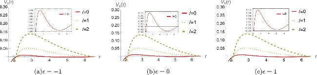
Figure 6. The effective potential Vs(r) for massless scalar field perturbations on black hole with fixed M = 1, Λ = 0.05 and Qm = 0.3. For these specific parameter values, the black hole event horizon is located at rh ≈ 2.115 26 and rc ≈ 6.442 26. Panels (a)–(c) correspond to ε = −1, ε = 0, and ε = 1, respectively. Each panel displays potentials for three values of the angular quantum number l = 0, 1, 2. Note the characteristic double-peak structure of the potential when l = 0. |
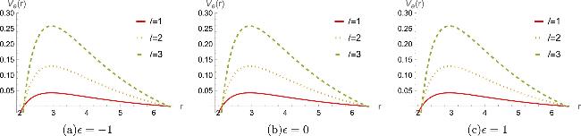
Figure 7. The effective potential Ve(r) for electromagnetic field perturbation on black hole with fixed M = 1, Λ = 0.05 and Qm = 0.3. Panels (a)–(c) correspond to ε = −1, ε = 0, and ε = 1, respectively. Each panel displays potentials for three values of the angular quantum number l = 1, 2, 3. The potential barrier height increases monotonically with both the multipole number l. |
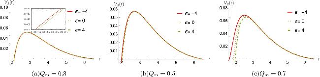
Figure 8. The effective potential Vs(r) for massless scalar field perturbation on black hole with fixed M = 1, Λ = 0.05 and l = 1. Panels (a)–(c) correspond to Qm = 0.3, Qm = 0.5, and Qm = 0.7, respectively. Each panel compares potentials for three coupling parameter values ε = −4, ε = 0, and ε = 4. The potential barrier height decreases monotonically with increasing ε. |
3.2. Electromagnetic field perturbation
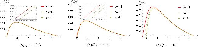
Figure 9. The effective potential Ve(r) for electromagnetic field perturbation on black hole with fixed M = 1, Λ = 0.05 and l = 1. Panels (a)–(c) correspond to Qm = 0.3, Qm = 0.5, and Qm = 0.7, respectively. Each panel compares potentials for three coupling parameter values ε = −4, ε = 0, and ε = 4. The potential barrier height decreases monotonically with increasing ε. |
4. Quasinormal mode frequencies
4.1. Asymptotic iteration method
4.2. 6th-order WKB method
4.3. Bernstein spectral method
5. Numerical results
5.1. Qm-dependence
Table 1. Comparison of fundamental QNFs (n = 0) for massless scalar field perturbations l = 0 obtained via the AIM, Bernstein spectral and WKB method. The parameters are fixed as M = 1, Λ = 0.05, ε = 0, ± 1 and Qm varies from 0.3 to 0.7. The parameter ϵ1 represents relative errors between AIM and Bernstein methods, ϵ2 represents relative errors between AIM and WKB methods. |
| ε | Qm | AIM | Bernstein spectral | ϵ1(%) | WKB | ϵ2(%) |
|---|---|---|---|---|---|---|
| 1 | 0.3 | 0.0755244 − 0.0996825i | 0.0754839 − 0.0996719i | 0.033532 | 0.0703929 − 0.0992877i | 4.1153 |
| 0.5 | 0.0799900 − 0.1015850i | 0.0799338 − 0.1015621i | 0.046942 | 0.0760739 − 0.0984478i | 3.8808 | |
| 0.7 | 0.0872094 − 0.1055948i | 0.0870846 − 0.1055414i | 0.099110 | 0.0927763 − 0.0944930i | 9.0684 | |
| | ||||||
| 0 | 0.3 | 0.0761242 − 0.0999622i | 0.0755935 − 0.099640i | 0.49392 | 0.0711911 − 0.0982916i | 4.1452 |
| 0.5 | 0.0803893 − 0.101386i | 0.0800 − 0.1013i | 0.46392 | 0.0762451 − 0.0995951i | 3.4893 | |
| 0.7 | 0.0874256 − 0.103788i | 0.0870 − 0.1040i | 0.35025 | 0.0840822 − 0.10198i | 2.8011 | |
| | ||||||
| −1 | 0.3 | 0.0755758 − 0.0996304i | 0.0755 − 0.0996i | 0.076028 | 0.0697726 − 0.100461i | 4.6880 |
| 0.5 | 0.0800608 − 0.100936i | 0.0800631 − 0.101291i | 0.27597 | 0.0768723 − 0.0999537i | 2.5896 | |
| 0.7 | 0.0874665 − 0.101225i | 0.0874479 − 0.101187i | 0.031672 | 0.0883847 − 0.0975922i | 2.8012 | |
Table 2. The fundamental QNFs (n = 0) of scalar perturbations and electromagnetic perturbations l = 1 for various ε and Qm. Other parameters are set to M = 1 and Λ = 0.05. The parameter ϵ2 represents relative errors between AIM and WKB methods. |
| Scalar perturbation | Electromagnetic perturbation | ||||||
|---|---|---|---|---|---|---|---|
| ε | Qm | AIM | WKB | ϵ2(%) | AIM | WKB | ϵ2(%) |
| 1 | 0.3 | 0.211816 − 0.0777350i | 0.211845 − 0.0777674i | 0.019117 | 0.191863 − 0.0707426i | 0.191835 − 0.0708107i | 0.036162 |
| 0.5 | 0.223456 − 0.0801152i | 0.0845594 − 0.109569i | 0.011044 | 0.201987 − 0.0731151i | 0.201913 − 0.0732115i | 0.056637 | |
| 0.7 | 0.242213 − 0.0845578i | 0.24207 − 0.084608i | 0.058903 | 0.218185 − 0.0775617i | 0.217855 − 0.0777876i | 0.17296 | |
| | |||||||
| 0 | 0.3 | 0.2118342 − 0.0777156i | 0.2118612 − 0.0777493i | 0.019140 | 0.1918838 − 0.0707257i | 0.191852 − 0.0707951i | 0.037424 |
| 0.5 | 0.2236277 − 0.0799076i | 0.2236487 − 0.0799311i | 0.013271 | 0.2021921 − 0.0729303i | 0.202161 − 0.0730071i | 0.038590 | |
| 0.7 | 0.2431877 − 0.0832337i | 0.2432030 − 0.0832420i | 0.0067756 | 0.2194009 − 0.0763619i | 0.219372 − 0.0764423i | 0.036808 | |
| | |||||||
| −1 | 0.3 | 0.211852 − 0.0776963i | 0.21188 − 0.0777303i | 0.019446 | 0.191904 − 0.0707087i | 0.191882 − 0.0707742i | 0.033769 |
| 0.5 | 0.22384 − 0.0797129i | 0.22384 − 0.0797129i | 0.018775 | 0.202397 − 0.0727402i | 0.20241 − 0.0727948i | 0.026132 | |
| 0.7 | 0.244093 − 0.0817178i | 0.244256 − 0.0815949i | 0.079390 | 0.220598 − 0.0749383i | 0.22087 − 0.0747863i | 0.13340 | |
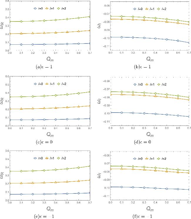
Figure 10. Variation of scalar fundamental QNFs (n = 0) with respect to the magnetic charge Qm for black hole with fixed mass M = 1 and cosmological constant Λ = 0.05. Panels (a), (b) correspond to coupling parameter ε = 1, (c), (d) to ε = 0, and (e), (f) to ε = −1. In each panel, curves for angular quantum numbers l = 0, 1, 2 are shown. For all coupling parameters considered, both Re(ω) and ∣Im(ω)∣ increase monotonically with growing magnetic charge Qm. |
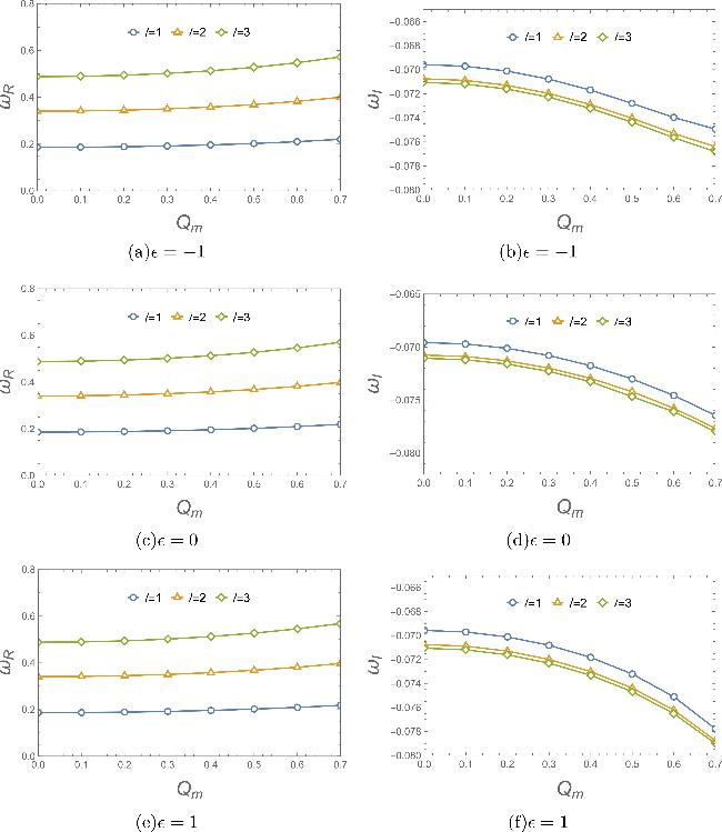
Figure 11. Variation of electromagnetic fundamental QNFs (n = 0) with respect to the magnetic charge Qm for black hole with fixed mass M = 1 and cosmological constant Λ = 0.05. Panels (a), (b) correspond to coupling parameter ε = −1, (c), (d) to ε = 0, and (e), (f) to ε = 1. In each panel, curves for angular quantum numbers l = 1, 2, 3 are shown. For all coupling parameters considered, both Re(ω) and ∣Im(ω)∣ increase monotonically with growing magnetic charge Qm. |
5.2. Λ-dependence
Table 3. The fundamental QNFs (n = 0) of scalar perturbations and electromagnetic perturbations l = 1 for various ε and Λ. Other parameters are set to M = 1 and Qm = 0.3. The parameter ϵ2 represents relative errors between AIM and WKB methods. |
| Scalar field perturbation | Electromagnetic field perturbation | ||||||
|---|---|---|---|---|---|---|---|
| ε | Λ | AIM | WKB | ϵ2(%) | AIM | WKB | ϵ2(%) |
| 1 | 0.01 | 0.281768 − 0.0951460i | 0.281735 − 0.0952336i | 0.031390 | 0.241923 − 0.0891115i | 0.24182 − 0.0892346i | 0.062358 |
| 0.05 | 0.211816 − 0.07773500i | 0.211845 − 0.0777674i | 0.019121 | 0.191863 − 0.0707426i | 0.191835 − 0.0708107i | 0.036163 | |
| 0.07 | 0.171217 − 0.0645797i | 0.171236 − 0.0646951i | 0.063913 | 0.160089 − 0.0591985i | 0.160138 − 0.059216i | 0.030115 | |
| | |||||||
| 0 | 0.01 | 0.281779 − 0.0951194i | 0.281753 − 0.095204i | 0.029778 | 0.241944 − 0.0890852i | 0.241854 − 0.0892002i | 0.056664 |
| 0.05 | 0.211834 − 0.0777157i | 0.211861 − 0.0777493i | 0.019143 | 0.191884 − 0.0707257i | 0.191852 − 0.0707951i | 0.037424 | |
| 0.07 | 0.171239 − 0.0645665i | 0.171249 − 0.0646861i | 0.065575 | 0.160111 − 0.0591870i | 0.160065 − 0.05924i | 0.041105 | |
| | |||||||
| −1 | 0.01 | 0.281791 − 0.0950926i | 0.281771 − 0.0951741i | 0.028222 | 0.241966 − 0.0890587i | 0.24189 − 0.0891654i | 0.050760 |
| 0.05 | 0.211852 − 0.0776963i | 0.21188 − 0.0777303i | 0.019450 | 0.191904 − 0.0707087i | 0.191879 − 0.0707755i | 0.034891 | |
| 0.07 | 0.171260 − 0.0645533i | 0.171295 − 0.0646648i | 0.063687 | 0.160132 − 0.0591754i | 0.160085 − 0.0592292i | 0.041846 | |
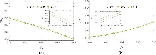
Figure 12. Variation of scalar fundamental QNFs, (n = 0) with respect to the cosmological constant Λ for black hole with fixed M = 1, Qm = 0.3 and l = 1. Panels (a) and (b) display Re(ω) and ∣Im(ω)∣, respectively. The curves correspond to different coupling parameters: ε = 1 (blue), ε = 0 (orange), and ε = −1 (green). As Λ increases, both Re(ω) and ∣Im(ω)∣ decrease monotonically. |
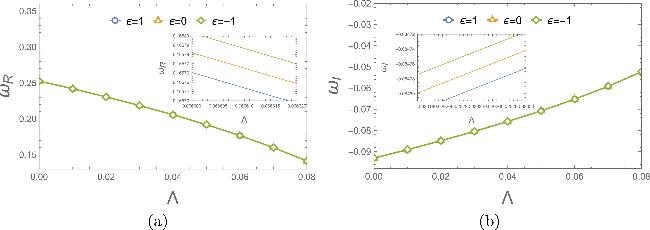
Figure 13. Variation of electromagnetic fundamental QNFs, (n = 0) with respect to the cosmological constant Λ for black hole with fixed M = 1, Qm = 0.3 and l = 1. Panels (a) and (b) display Re(ω) and ∣Im(ω)∣, respectively. The curves correspond to different coupling parameters: ε = 1 (blue), ε = 0 (orange), and ε = −1 (green). As Λ increases, both Re(ω) and ∣Im(ω)∣ decrease monotonically. |
5.3. ε-dependence
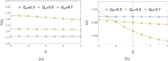
Figure 14. Variation of scalar fundamental QNFs (n = 0) with respect to the nonlinear coupling parameter ε for black hole with fixed M = 1, Λ = 0.05 and l = 1. Panel (a) displays Re(ω) and panel (b) shows Im(ω). Each panel compares results for three different magnetic charges: Qm = 0.3 (blue), Qm = 0.5 (orange), and Qm = 0.7 (green). For smaller magnetic charges (Qm = 0.3, 0.5), both Re(ω) and ∣Im(ω)∣ exhibit minimal dependence on ε. However, for the larger magnetic charge (Qm = 0.7), increasing ε leads to a moderate decrease in both oscillation frequency and damping rate. |
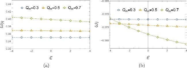
Figure 15. Variation of electromagnetic fundamental QNFs (n = 0) with respect to the nonlinear coupling parameter ε for black hole with fixed M = 1, Λ = 0.05 and l = 1. Panel (a) displays Re(ω) and panel (b) shows Im(ω). Each panel compares results for three different magnetic charges: Qm = 0.3 (blue), Qm = 0.5 (orange), and Qm = 0.7 (green). For smaller magnetic charges (Qm = 0.3, 0.5), both Re(ω) and ∣Im(ω)∣ exhibit minimal dependence on ε. However, for the larger magnetic charge (Qm = 0.7), increasing ε leads to a moderate decrease in both oscillation frequency and damping rate. |
6. The greybody factor
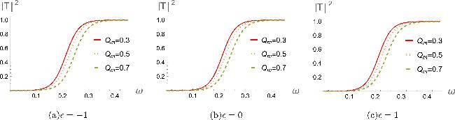
Figure 16. Greybody factors ∥T(ω)∥2 for massless scalar field perturbations on black hole with fixed M = 1, Λ = 0.05, and l = 1. The three panels display results for different coupling parameters ε = −1, 0, +1. Each panel compares the transmission probabilities for three values of magnetic charge Qm = 0.3 (red), Qm = 0.5 (orange), and Qm = 0.7 (green). Notably, the greybody factor decreases monotonically with increasing magnetic charge Qm for all coupling parameters. |
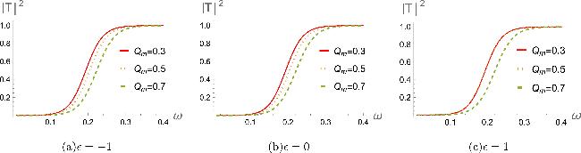
Figure 17. Greybody factors ∥T(ω)∥2 for electromagnetic field perturbations on black hole with fixed M = 1, Λ = 0.05, and l = 1. The three panels display results for different coupling parameters ε = −1, 0, +1. Each panel compares the transmission probabilities for three values of magnetic charge Qm = 0.3 (red), Qm = 0.5 (orange), and Qm = 0.7 (green). Notably, the greybody factor decreases monotonically with increasing magnetic charge Qm for all coupling parameters. |
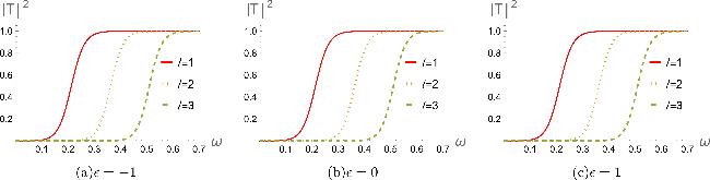
Figure 18. Greybody factors ∥T(ω)∥2 for massless scalar field perturbations on black hole with fixed M = 1, Λ = 0.05, and Qm = 0.3. The three panels display results for different coupling parameters ε = −1, 0, +1. Each panel compares the transmission probabilities for three values of l = 1 (red), l = 2 (orange), and l = 3 (green). Notably, the greybody factor decreases monotonically with increasing l for all coupling parameters. |
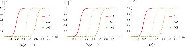
Figure 19. Greybody factors ∥T(ω)∥2 for electromagnetic field perturbations on black hole with fixed M = 1, Λ = 0.05, and Qm = 0.3. The three panels display results for different coupling parameters ε = −1, 0, +1. Each panel compares the transmission probabilities for three values of l = 1 (red), l = 2 (orange), and l = 3 (green). Notably, the greybody factor decreases monotonically with increasing l for all coupling parameters. |
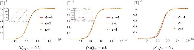
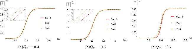
Figure 20. Greybody factors ∥T(ω)∥2 for massless scalar field perturbations on black hole with fixed M = 1, Λ = 0.05, and l = 1. The three panels display results for different magnetic charges Qm = 0.3, 0.5, 0.7. Each panel compares the transmission probabilities for three values of coupling parameters ε = −4 (red), ε = 0 (orange), and ε = 4 (green). Notably, the greybody factor increases monotonically with increasing ε for all magnetic charges. |
Figure 21. Greybody factors ∥T(ω)∥2 for electromagnetic field perturbations on black hole with fixed M = 1, Λ = 0.05, and l = 1. The three panels display results for different magnetic charges Qm = 0.3, 0.5, 0.7. Each panel compares the transmission probabilities for three values of coupling parameters ε = −4 (red), ε = 0 (orange), and ε = 4 (green). Notably, the greybody factor increases monotonically with increasing ε for all magnetic charges. |