


1. Introduction
Bosonic particles with significant beyond mean-field interaction can undergo a phase transition to a Bose–Einstein condensate (BEC) at an extremely low temperature [1]. This BEC provides a platform to realize a special phase, called quantum droplet (QD) [2, 3]. The QDs are self-bound states that occur in BECs due to the balance between quantum fluctuation (Lee–Huang–Yang correction) and mean-field interaction. The effect of quantum fluctuation is enhanced by the dipole-dipole interaction (DDI). QDs have been experimentally realized both in non-dipolar BECs and dipolar BECs of dysprosium (Dy), chromium (Cr) and erbium (Er) atoms [4–10]. In the latter case, large magnetic dipole moments of the atoms play prominent roles in the formation of QDs.
A variety of interesting phenomena has come into existence due to the interplay between long-range anistropic dipole-dipole interaction (DDI) and contact interactions. This includes anisotropic superfluidity [11–13], supersolid states [14, 15] and appearance of roton excitation [16–19]. Due to the presence of the roton excitation, a dipolar BEC gives rise to distinct phases, namely, vortices and supersolid [20–23]. Dipolar ground state of molecules are also realized experimentally by Ni et al [24].
In the quantum droplet, matter density is high and thus one of the possible effects that comes into play is the three-body recombination. The inclusion of three-body loss induces dissipative dynamics that crucially affects the droplet's behavior [25]. More specifically, as atoms are lost due to three-body recombination, an imbalance between the quantum fluctuation and mean-field interaction occurs. This results in an expansion of droplets and eventually destabilizes if the number of atoms drops below a critical value. This recombination process leads to a density-dependent loss of atoms and renders the droplets intrinsically finite-lived. To compensate this dissipation, one may introduce external atomic feeding, representing a continuous supply of atoms into the system. Thus the stability of a quantum droplet (QD) is achieved when the gain from feeding precisely counterbalances the density-dependent loss. The dissipation-managed dynamics of the QDs in optical lattices are independent of the initial norm of the condensate but depends on loss and gain parameters [26]. There are several attempts to understand the properties of Bose–Einstein condensates with two- and three-body inelastic processes in the absence of quantum fluctuations [27, 28].
Our objective in this paper is to study static and dynamical properties of QDs in the presence of three-body loss and external feeding in harmonically trapped Bose–Einstein condensation. More specifically, we consider a spherically symmetric trap and find an effective potential for the width of the QDs. It is seen that the width of a droplet corresponding to the potential minimum is significantly affected in the presence of three-body losses. Particularly, the width of a QD at the potential minimum is larger for stronger values of three-body loss. The time evolution of the density profile of a QD shows that the amplitude of oscillation of the width of a droplet decreases with time due to the loss of atoms. However, the width of a droplet is augmented if the condensate is continuously fed by an external source. The stability of a QD is found to depend sensitively on the relative strength of the three-body recombination and external feeding. In the context of a matter-wave soliton, the effects of a three-body loss on the dynamics of a soliton have been studied by several authors and examined the region of stability in the presence of external feeding [28, 29]. The alimentation of atoms from an external source compensates for the loss and results in dynamically-stabilized solitons [30].
In section 2 , we present a theoretical model to describe the dynamics of a quantum droplet in BECs with a view to examine the effects of a three-body loss and external feeding. Particularly, we present a variational model for dissipative systems and construct an effective potential for the droplet. In section 3 , we study the dynamics of both sharp- and flat-top QDs in the absence of a three-body loss. In section 4 , we consider the effects of the loss of atoms due to the three-body recombination and show that the dissemination of the density profile of the droplet can be arrested by feeding the condensates from an external source. In section 5 , we present the fixed point analysis to check the linear stability of the droplet. In section 6 , we make some concluding remarks.
2. Theoretical formulation for QD dynamics
We consider the dynamics of QDs in BECs with three-body loss and external feeding by the following Gross–Pitaevskii equation (GPE) [29, 31–38].1 ), Vext(r) represents trapping potential.
$\begin{eqnarray}\begin{array}{rc}{\rm{i}}\hslash \frac{\partial {\rm{\Psi }}}{\partial t} & =-\frac{{\hslash }^{2}}{2m}{{\rm{\nabla }}}^{2}{\rm{\Psi }}+g| {\rm{\Psi }}{| }^{2}{\rm{\Psi }}-{g}_{1}| {\rm{\Psi }}{| }^{3}{\rm{\Psi }}\\ & +{V}_{{\rm{ext}}}({\boldsymbol{r}}){\rm{\Psi }}-\frac{{\rm{i}}\hslash {L}_{3}}{2}| {\rm{\Psi }}{| }^{4}{\rm{\Psi }}+\frac{{\rm{i}}\gamma }{2}{\rm{\Psi }},\end{array}\end{eqnarray}$
with ${g}_{1}=\frac{128\sqrt{\pi }{\hslash }^{2}}{3m}{a}_{s}^{\frac{5}{2}}$. Here, ${\rm{\Psi }}\left({\boldsymbol{r}},t\right)$ is the order parameter of the condensate and as is the atomic scattering length. The parameters g, g1, L3 and γ stand for the strengths of mean-field interaction, quantum fluctuation, coefficient of three-body recombination, and external feeding coefficient respectively. In equation (We take spherically symmetric $\left(l=0\right)$ trap with ${V}_{{\rm{ext}}}({\boldsymbol{r}})=\frac{1}{2}m{\omega }^{2}{r}^{2}$ and rewrite equation (1 ) using ${\rm{\Psi }}\left({\boldsymbol{r}},t\right)\,=\psi \left(r,t\right){Y}_{l}^{{m}^{{\prime} }}\left(\theta ,\phi \right)$ as 2 ) becomes dimensionless. Here ω, l0 are the frequency and characteristic length of transverse harmonic trap. In terms of these variables, equation (2 ) is given by 3 ) are given by 3 ).
$\begin{eqnarray}\begin{array}{rc}{\rm{i}}\hslash \frac{\partial \psi }{\partial t} & =-\frac{{\hslash }^{2}}{2m}\left(\frac{{\partial }^{2}}{\partial {r}^{2}}+\frac{2}{r}\frac{\partial }{\partial r}\right)\psi +g| \psi {| }^{2}\psi -{g}_{1}| \psi {| }^{3}\psi \\ & +\frac{1}{2}m{\omega }^{2}{r}^{2}\psi -\frac{{\rm{i}}\hslash {L}_{3}}{2}| \psi {| }^{4}\psi +\frac{{\rm{i}}\gamma }{2}\psi .\end{array}\end{eqnarray}$
We defined the following variables, $\begin{eqnarray*}{l}_{0}=\sqrt{\frac{\hslash }{m\omega }},\,\,\tilde{r}=\frac{r}{{l}_{0}},\,\,\,\tilde{t}=\omega t\,\,{\rm{and}}\,\,\tilde{\psi }=\psi {l}_{0}^{\frac{3}{2}},\end{eqnarray*}$
such that equation ( $\begin{eqnarray}\begin{array}{rc}{\rm{i}}\frac{\partial \psi }{\partial t} & +\frac{1}{2}\left(\frac{{\partial }^{2}}{\partial {r}^{2}}+\frac{2}{r}\frac{\partial }{\partial r}\right)\psi -g| \psi {| }^{2}\psi +{g}_{1}| \psi {| }^{3}\psi \\ & -\frac{1}{2}{r}^{2}\psi +\frac{{\rm{i}}{L}_{3}}{2}| \psi {| }^{4}\psi -\frac{{\rm{i}}\gamma }{2}\psi =0.\end{array}\end{eqnarray}$
The parameters in equation ( $\begin{eqnarray*}\begin{array}{r}\tilde{g}=\frac{g}{\hslash \omega {l}_{0}^{3}},\,\,\,\,\,\,{\tilde{g}}_{1}=\frac{{g}_{1}}{\hslash \omega {l}_{0}^{9/2}},\\ \,\,\,{\tilde{L}}_{3}=\frac{{L}_{3}}{\omega {l}_{0}^{15/2}},\,\,\,{\tilde{V}}_{{\rm{ext}}}=\frac{{V}_{{\rm{ext}}}}{\hslash \omega },\tilde{\gamma }=\frac{\gamma }{\hslash \omega }.\end{array}\end{eqnarray*}$
Note that we have omitted tildes for convenience of presentation in equation (The Lagrangian density corresponding to equation (3 ) is given by 3 ) for$\frac{\delta {{ \mathcal L }}_{{ \mathcal R }}}{\delta {\psi }^{* }}={\rm{i}}\left(\frac{{L}_{3}}{2}| \psi {| }^{4}\psi -\frac{\gamma }{2}\psi \right)$.
$\begin{eqnarray}\begin{array}{rc}{ \mathcal L } & =\frac{{\rm{i}}}{2}\left(\psi \frac{\partial {\psi }^{\star }}{\partial t}-{\psi }^{\star }\frac{\partial \psi }{\partial t}\right)+\frac{1}{2}{\left|\frac{\partial \psi }{\partial r}\right|}^{2}+\frac{g}{2}{\left|\psi \right|}^{4}\\ & -\frac{2{g}_{1}}{5}{\left|\psi \right|}^{5}+\frac{1}{2}{r}^{2}{\left|\psi \right|}^{2},\end{array}\end{eqnarray}$
and $\begin{eqnarray}{{ \mathcal L }}_{{ \mathcal R }}=-\frac{{\rm{i}}{L}_{3}}{6}{\left|\psi \left(r,t\right)\right|}^{6}+\frac{{\rm{i}}\gamma }{2}| \psi {| }^{2}.\end{eqnarray}$
Here ${ \mathcal L }$ and ${{ \mathcal L }}_{{ \mathcal R }}$ represent respectively Lagrangian densities for conservative and dissipative parts of the system. One can check that $\frac{\delta }{\delta {\psi }^{* }}\left({ \mathcal L }+{{ \mathcal L }}_{{ \mathcal R }}\right)=0$ gives equation (We know that BECs in presence of quantum fluctuation permit both sharp- and flat-top bell-shaped QD solutions [39–41]. Particularly, equation (1 ) in the limits of γ → 0 and L3 → 0 gives exact bell-shaped solution. Thus we employ the following super-Gaussian trial function [42, 43],
$\begin{eqnarray}\psi (r,t)=A{{\rm{e}}}^{\left(-\frac{1}{2}{\left(\frac{r}{w}\right)}^{2\eta }+ib{r}^{2}+{\rm{i}}\phi \right)},\end{eqnarray}$
which gives sharp- and flat- top QDs for the smaller and larger values of η. Here A(t), b(t), w(t) and φ(t) are the variational parameters denoting the amplitude, chirp, width and initial phase, respectively. Understandably, the effects of the three-body recombination and external feeding come through variational parameters. The norm of the system is given by $\begin{eqnarray}N=4\pi {\int }_{0}^{\infty }{r}^{2}{\left|\psi \right|}^{2}{\rm{d}}r=\frac{4\pi {A}^{2}{w}^{3}}{2\eta }{\rm{\Gamma }}\left(\frac{3}{2\eta }\right),\end{eqnarray}$
is a conserved quantity which is related to the actual number of atoms in a droplet.In order to find the values of variational parameters for the dissipative system, we first write the averaged Lagrangian using $L=4\pi {\int }_{0}^{\infty }{r}^{2}{ \mathcal L }{\rm{d}}r$ for the conservative part 9 ), we use equation (7 ) to replace A by w and N. The equations for the variational parameter yj can be derived by the use of the following Euler-Lagrangian equation [44–46].6 ) and (9 ) in equation (10 ), yield the following equations of variational parameters. For yj = w, we get 10 ) gives 11 ) and (12 ), we get 15 ).
$\begin{eqnarray}L=N\dot{\phi }+\frac{N{\rm{\Gamma }}\left(\frac{5}{2\eta }\right)}{{\rm{\Gamma }}\left(\frac{3}{2\eta }\right)}{w}^{2}\left(\dot{b}+2{b}^{2}\right)+G\left(\eta ,w,N\right),\end{eqnarray}$
where $\begin{eqnarray}G\left(\eta ,w,N\right)=\frac{{G}_{0}}{{w}^{2}}+\frac{g{G}_{1}}{{w}^{3}}-\frac{{g}_{1}{G}_{2}}{{w}^{\frac{9}{2}}}+{G}_{3}{w}^{2},\end{eqnarray}$
with $\begin{eqnarray*}\begin{array}{r}{G}_{0}=\frac{{\eta }^{2}N{\rm{\Gamma }}\left(2+\frac{1}{2\eta }\right)}{2{\rm{\Gamma }}\left(\frac{3}{2\eta }\right)},\,\,\,{G}_{1}=\frac{\eta {N}^{2}}{4\pi {2}^{3/2\eta }{\rm{\Gamma }}\left(\frac{3}{2\eta }\right)},\\ {G}_{2}=\frac{2{N}^{5/2}}{5{\left(\frac{5}{2}\right)}^{\frac{3}{2\eta }}}{\left(\frac{2\eta }{4\pi {\rm{\Gamma }}\left(\frac{3}{2\eta }\right)}\right)}^{3/2},{G}_{3}=\frac{N{\rm{\Gamma }}\left(\frac{5}{2\eta }\right)}{2{\rm{\Gamma }}\left(\frac{3}{2\eta }\right)}.\end{array}\end{eqnarray*}$
In writing equation ( $\begin{eqnarray}\frac{\partial L}{\partial {y}_{j}}-\frac{{\rm{d}}}{{\rm{d}}t}\left(\frac{\partial L}{\partial {y}_{j}^{{\prime} }}\right)=4\pi \int {r}^{2}\left[R\frac{\partial {\psi }^{* }}{\partial {y}_{j}}+{R}^{* }\frac{\partial \psi }{\partial {y}_{j}}\right]{\rm{d}}r,\end{eqnarray}$
with $R=-\frac{\delta {{ \mathcal L }}_{{ \mathcal R }}}{\delta {\psi }^{* }}$, the Rayleigh dissipative function. Here, yj = A, w, b, φ while ${y}_{j}^{{\prime} }$ stands for their time derivatives. Substitutions of equations ( $\begin{eqnarray}\dot{b}=-2{b}^{2}-\frac{{\rm{\Gamma }}\left(\frac{3}{2\eta }\right)}{2N{\rm{\Gamma }}\left(\frac{5}{2\eta }\right)w}\frac{\partial G}{\partial w}.\end{eqnarray}$
For yj = b, equation ( $\begin{eqnarray}\dot{w}=2bw-\alpha \left(\frac{{N}^{2}}{{w}^{5}}\right),\end{eqnarray}$
where $\alpha =\frac{{L}_{3}{\eta }^{2}}{8{\pi }^{2}\,\,{3}^{\left(\frac{5}{2\eta }\right)}{\rm{\Gamma }}{\left(\frac{3}{2\eta }\right)}^{2}}$. Similarly, for yj = φ, the evolution of φ gives rise to $\begin{eqnarray}\frac{{\rm{d}}N}{{\rm{d}}t}=-K{N}^{3}+\gamma N.\end{eqnarray}$
Here, $K=\frac{{\eta }^{2}{L}_{3}}{4{\pi }^{2}{w}^{6}{3}^{\frac{3}{2\eta }}{\left({\rm{\Gamma }}\left(\frac{3}{2\eta }\right)\right)}^{2}}=\frac{2\alpha {3}^{1/\eta }}{{w}^{6}}$. Combining equations ( $\begin{eqnarray}\ddot{w}=-\frac{{\rm{\Gamma }}\left(\frac{3}{2\eta }\right)}{N{\rm{\Gamma }}\left(\frac{5}{2\eta }\right)}\frac{\partial G}{\partial w}-\alpha \left[\frac{2{N}^{2}}{{w}^{5}}\left(\gamma -K{N}^{2}-4b\right)+\frac{5\alpha {N}^{4}}{{w}^{11}}\right].\end{eqnarray}$
This is a second-order nonlinear differential equation of width. Using $\ddot{w}=-\frac{{\rm{d}}U}{{\rm{d}}w}$, we find the following effective potential for a QD. $\begin{eqnarray}U=\frac{{\rm{\Gamma }}\left(\frac{3}{2\eta }\right)}{N{\rm{\Gamma }}\left(\frac{5}{2\eta }\right)}G+\zeta ,\end{eqnarray}$
with $\zeta =\alpha \left[\frac{{N}^{2}}{2{w}^{4}}\left(K{N}^{2}+4b-\gamma \right)-\frac{\alpha {N}^{4}}{2{w}^{10}}\right]$. Understandably, U gives an effective potential for a droplet in the presence of a three-body recombination and atomic feeding. In the following, we analyze the effective potential and study the dynamics of QDs with the help of equation (3. Dynamics of QDs without three-body loss
In the absence of three-body loss (i,e., L3 = 0) and atomic feeding (i,e.,γ = 0), the number of particles in the system is strictly conserved. One can verify from equation (13 ) that N is constant for K = γ = 0. Under this circumstance, equation (14 ) turns out to be
$\begin{eqnarray}\ddot{w}=-\frac{{\rm{\Gamma }}\left(\frac{3}{2\eta }\right)}{{\rm{\Gamma }}\left(\frac{5}{2\eta }\right)}\frac{\partial G}{\partial w}=-\frac{{\rm{d}}U\left(w\right)}{{\rm{d}}w},\end{eqnarray}$
and the corresponding effective potential is obtained as $\begin{eqnarray}U\left(w\right)=\frac{{\rm{\Gamma }}\left(\frac{3}{2\eta }\right)}{N{\rm{\Gamma }}\left(\frac{5}{2\eta }\right)}G.\end{eqnarray}$
This gives effective potentials for both sharp- and flat-top QDs in the absence of a three-body recombination and external feeding.Figure 1 portrays an effective potential of width and density profile for a flat-top QD (left and right panels). It shows that, due to the competition between quantum fluctuations (LHY correction) and mean-field interactions, a minimum appears at w = wm in the effective potential indicating a possibility for the existence of a stable quantum droplet of width wm. For a sharp-top QD, we observe a similar behavior (figure 2). However, the width of a sharp-top QD is relatively smaller than that of a flat-top QD.
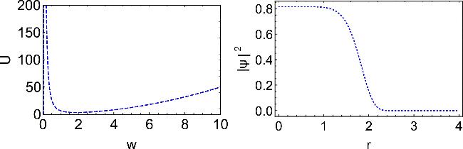
Figure 1. Left panel: U versus w curves of a flat-top QD for b = 1, g = 0.1, g1 = 0.5. U is minimum at wm = 1.87507. Right panel: it gives density profiles of a QD with a width corresponding to the minimum of the effective potential. In both the panels, we take η = 4 and N = 20. |
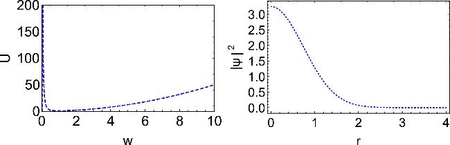
Figure 2. Left panel: U versus w curves of a sharp-top QD for b = 1, g = 0.1, g1 = 0.5, potential minimum occurs at wm = 1.03787. Right panel: it gives the density profile of a QD with a width corresponding to minimum of the effective potential. In both the panels, we take η = 1.01 and N = 20. |
With a view to get the dynamics of the width of a flat-top QD, we solve equation (16 ) and use equations (6 ) and (7 ) to investigate the dynamics of the density profile. The time evolution of the width of the flat-top QDs displayed in figure 3 shows that the values of the width oscillates below wm periodically with time if the initial width (wi) is taken greater than wm which corresponds to the potential minimum (top-left panel). We observe an opposite behavior if the initial width (wi) is taken relatively smaller than that of wm (top-right panel). The time variations of the density profiles of QDs for wi > wm and wi < wm are given in the bottom panel. It shows that the amplitude of the density profiles of QDs oscillate periodically in both the cases. We observe a similar variation of the width and density profile of a sharp-top QD for both wi > wm and wi < wm (figure 4).
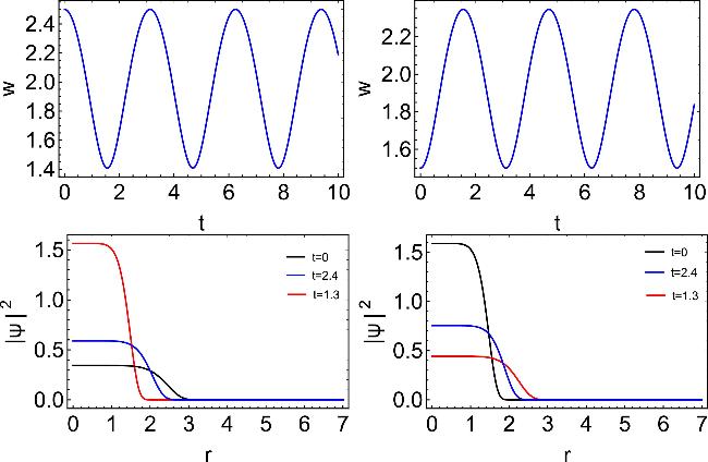
Figure 3. Top panel: variation of width with time of a flat-top QD for wi > wm (left panel) and wi < wm (right panel). For each case, we take b = 1, g = 0.1, g1 = 0.0005, N = 20 and η = 4. Bottom panel: density profiles of QD at different times. |
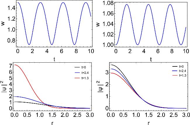
Figure 4. Top panel: variation of width of a sharp-top QD for wi > wm (left panel) and wi < wm (right panel). For each case, we take b = 1, g = 0.1, g1 = 0.0005 and η = 1.01. Bottom panel: the evolution of the density profile of a sharp-top QD at different times. |
4. Effects of three-body loss and external feeding on QDs
A Bose–Einstein condensate in the QD phase may suffer from the loss of atoms due to three-body inelastic collision since the atom density in this phase is relatively high. Therefore, it is quite important to incorporate three-body loss to find the effect of dissipation on the dynamical behavior of QDs. We note that the interplay between the contact interaction and LHY correction determines the stability of a QD. The three-body loss causes an imbalance and can result in changes in the dynamics of QDs. More specifically, it can significantly influence the condensate's evolution, potentially leading to density depletion and causing shape modifications, or can even result in a collapse in certain regimes.
In the presence of three-body loss, the variation of the number of atoms obtained from equation (13 ) with γ = 0 is given by 18 ) that the total number of atoms in the condensate decreases with time, and thus it can affect the overall properties and stability of the quantum droplets (blue curve, figure 5).
$\begin{eqnarray}N\left(t\right)=\frac{{N}_{0}}{\sqrt{\left(1+2{N}_{0}\int K(t)dt\right)}}.\end{eqnarray}$
Here, N0 is the number of particles of the system at t = 0. It is obvious from equation (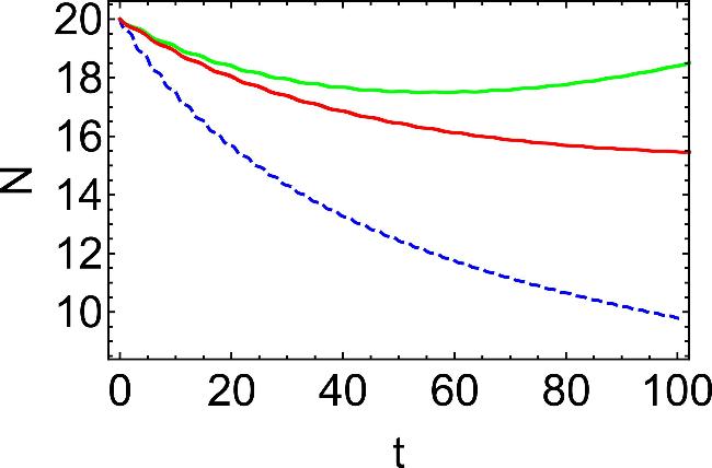
Figure 5. Variation of number of particles in presence of both three-body loss and external feeding of a flat for η = 4 and L3 = 25. Here, the blue, red and green curves are drawn for γ = 0, γ = 0.008 and γ = 0.016 respectively. For each curve, we take b = 1, g = 0.1, g1 = 0.0005 and N = 20. |
The effective potential in presence of three-body loss is shown in figure 6. Here, the potential becomes minimum at a particular value of width (wm) for a chosen value of three-body loss (L3). However, the value of wm increases as L3 increases. This clearly indicates that, as the mean-field interaction decreases with the loss of atoms, an imbalance occurs leading to the increase of width. More specifically, the interplay between the repulsive interaction due to LHY correction and attractive mean-field interaction results in a QD with relatively larger width.
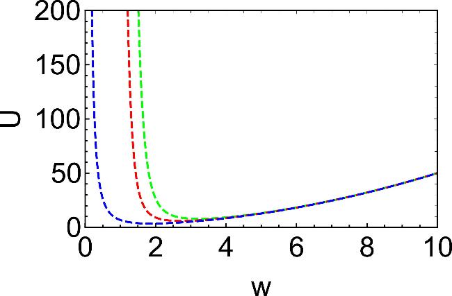
Figure 6. U versus w curves of a flat-top for different values of three-body loss coefficient. Here, blue, red and green curves are drawn for L3 = 0.00001 (wm = 1.87508), L3 = 5 (wm = 2.72248), and L3 = 15 (wm = 3.20561) respectively. For each curve, we take b = 1, g = 0.1, g1 = 0.0005, η = 4 and N0 = 20. |
The time evolution of width (w) displayed in figure 7 clearly shows that the value of the width of a QD oscillates and the amplitude of oscillation decreases with time due to the loss of atoms. This causes temporal variations of amplitude of the density profile (∣ψ∣2). Particularly, the top of the QD becomes gradually flat and the amplitude of ∣ψ∣2 diminishes with time (right panel). Thus the three-body loss can result in the disappearance of the droplet from the trap. However, the droplet can persist in a trap if it is properly fed from an external source. Particularly, we can add atoms externally by linear feeding such that the loss of atoms due to three-body recombination is compensated.
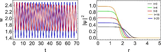
Figure 7. Left panel: the variation of the width with the time of the flat-top for η = 4 and γ = 0. Here, blue and red curves are drawn for L3 = 0 and L3 = 0.3 respectively. For each case, we take b = 1, g = 0.1, g1 = 0.0005 and N = 20. Right panel: the variation of the density profile at different times corresponding to the red curve. |
In figure 5, we illustrate the interplay between the three-body loss and external feeding for a fixed value of quantum fluctuation. In the absence of external feeding (blue curve), the number of particles decreases over time due to the three-body recombination. When external feeding is introduced, these losses are partially or fully compensated. The green curve associated with a higher value of the feeding parameter(γ) shows a more effective compensation compared to the red curve where γ is relatively small. For an appropriate larger value of γ, the external feeding can counterbalance the loss induced by the three-body interactions.
The time evolution of width in presence of the three-body loss and external feeding shown in the left panel of figure 8, clearly reflect the fact that the decrease of maximum amplitude of width with time is arrested in the presence of external feeding and results in periodic variation of width without any attenuation for a relatively larger value of feeding. The effect of feeding on the density profile of a QD at a particular time confirms that the amplitude of the density profile increases as feeding increases.
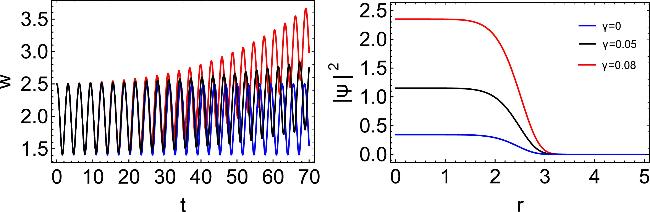
Figure 8. Left panel: the variation of width with time of flat-top for η = 4. Here, blue, black, and red curves are drawn for γ = 0, γ = 0.05 and γ = 0.08 respectively. For each curve, we take L3 = 0.000001, b = 1, g = 0.1, g1 = 0.0005 and N0 = 20. Right panel: the density profiles corresponding to each curve shown in the left panel at t = 25. |
5. Linear stability analysis of QD
We have seen that the loss of atoms from a QD can be compensated by externally feeding the condensate. However, this type of non-conservative contribution to the condensate can significantly affect the stability of a QD. Here, we consider a fixed point analysis to examine the linear stability of a QD. In order of this, we rewrite equations (11 ), (12 ), and (13 ) in terms of w and A as follows [28].
$\begin{eqnarray}\frac{{\rm{d}}}{{\rm{d}}t}\left({A}^{2}{w}^{3}\right)=-{c}_{00}{L}_{3}{A}^{6}{w}^{3}+\gamma {A}^{2}{w}^{3},\end{eqnarray}$
$\begin{eqnarray}\frac{{\rm{d}}w}{{\rm{d}}t}=2bw-{c}_{01}{L}_{3}{A}^{4}w,\end{eqnarray}$
$\begin{eqnarray}\frac{{\rm{d}}b}{{\rm{d}}t}=-2{b}^{2}+\frac{{c}_{0}}{{w}^{4}}-{c}_{1}\frac{{A}^{2}}{{w}^{2}}+{c}_{2}\frac{{A}^{3}}{{w}^{2}}-\frac{5}{4},\end{eqnarray}$
with $\begin{eqnarray*}{c}_{00}=\frac{1}{{3}^{\frac{3}{2\eta }}},\,\,\,{c}_{1}=\frac{3\eta g{\rm{\Gamma }}\left(\frac{3}{2\eta }\right)}{4{\rm{\Gamma }}\left(\frac{5}{2\eta }\right){2}^{\frac{3}{2\eta }}},\,\,\,\end{eqnarray*}$
$\begin{eqnarray*}{c}_{01}=\frac{0.5}{{3}^{\frac{5}{2\eta }}},\,\,\,\,{c}_{2}=\frac{3{g}_{1}{\rm{\Gamma }}\left(\frac{3}{2\eta }\right)}{5{\rm{\Gamma }}\left(\frac{5}{2\eta }\right){\left(\frac{5}{2}\right)}^{\frac{3}{2\eta }}}.\end{eqnarray*}$
It is now convenient to introduce new variables x = w2 and y = A2 and express equations (19 ) to (21 ) in terms of them. The above equations thus turn out to be 22 ) to (24 ) about the fixed point using transformation 32 ) is negative [28]. In figure 9, we take three different values of L3, (left panel) and plot the variation of real parts of root of equation (32 ) for different values of γ. It is seen that, for a given value of quantum fluctuation, the highest value of γ for the stability of a QD increases with the increase of L3 (left panel). For a given value of L3, the highest value of γ also increases with the increase of g1 (right panel). We see that the highest value of γ for a stable quantum droplet decreases as the quantum fluctuation decreases. Therefore, quantum fluctuation can oppose the loss due to the three-body recombination during the formation of stable QDs.
$\begin{eqnarray}{x}_{t}=4bx-2{C}_{01}{L}_{3}{y}^{2}x,\end{eqnarray}$
$\begin{eqnarray}{y}_{t}=-6by+{C}_{s}{L}_{3}{y}^{3}+\gamma y,\end{eqnarray}$
$\begin{eqnarray}{b}_{t}=-2{b}^{2}-\frac{{c}_{0}}{{x}^{2}}-\frac{{c}_{1}y}{x}+\frac{{c}_{2}{y}^{\frac{3}{2}}}{x}-\frac{5}{4}.\end{eqnarray}$
With a view to consider fixed point analysis, we set the time derivatives of xt, yt and bt equal to zero and obtain the following stable points of the system $\begin{eqnarray}{y}_{1s}=\pm \sqrt{\frac{\gamma }{{L}_{3}\left(3{c}_{01}-{c}_{s}\right)}},\end{eqnarray}$
$\begin{eqnarray}{b}_{1s}=\frac{{c}_{01}{L}_{3}{y}_{1s}^{2}}{2},\end{eqnarray}$
$\begin{eqnarray}{x}_{1s}=\frac{{c}_{2}{y}_{1s}^{\frac{3}{2}}-{c}_{1}{y}_{1s}\pm \sqrt{{\left({c}_{1}{y}_{1s}-{c}_{2}{y}_{1s}^{\frac{3}{2}}\right)}^{2}-{c}_{0}\left(8{b}_{1s}^{2}+5\right)}}{\left(4{b}_{1s}^{2}+2.5\right)}.\end{eqnarray}$
We linearize equations ( $\begin{eqnarray}x={x}_{1s}+{x}_{1},\,\,y={y}_{1s}+{y}_{1},\,\,\,b={b}_{1s}+{b}_{1},\end{eqnarray}$
taking x1, y1, b1 as much smaller than x1s, y1s, b1s respectively. The linearized equations are given by $\begin{eqnarray}\frac{{\rm{d}}{x}_{1}}{{\rm{d}}t}={a}_{1}{x}_{1}+{a}_{2}{y}_{1}+{a}_{3}{b}_{1},\end{eqnarray}$
$\begin{eqnarray}\frac{{\rm{d}}{y}_{1}}{{\rm{d}}t}={d}_{2}{y}_{1}+{d}_{3}{b}_{1},\end{eqnarray}$
and $\begin{eqnarray}\frac{{\rm{d}}{b}_{1}}{{\rm{d}}t}={e}_{1}{x}_{1}+{e}_{2}{y}_{1}+{e}_{3}{b}_{1}.\end{eqnarray}$
Here ${a}_{1}=\,4{b}_{1s}-2{c}_{01}{L}_{3}{y}_{1s}^{2},$ ${a}_{2}=-4{c}_{01}{L}_{3}{y}_{1s}{x}_{1s},$ ${a}_{3}=4{x}_{1s},$ ${d}_{2}=-6{b}_{1s}+3{y}_{1s}^{2}{c}_{s}{L}_{3}+\gamma ,$ ${d}_{3}=-6{y}_{1s},$ ${e}_{1}=\frac{2{c}_{0}}{{x}_{1s}^{3}}+\frac{{c}_{1}{y}_{1s}}{{x}_{1s}^{2}}\,-\frac{{c}_{2}{y}_{1s}^{\frac{3}{2}}}{{x}_{1s}},$ ${e}_{2}=-\frac{{c}_{1}}{{x}_{1s}}+\frac{3{c}_{2}{y}_{1s}^{\frac{1}{2}}}{2{x}_{1s}},$ ${e}_{3}=-4{b}_{1s}$. Understandably, x1, y1, and b1 give the solution of linearized system of equations. Taking these solutions of the form ≈ert, we get the characteristic equation [28] $\begin{eqnarray}{r}^{3}-{\alpha }_{1}{r}^{2}+{\alpha }_{2}r+{\alpha }_{3}=0,\end{eqnarray}$
where $\begin{eqnarray*}{\alpha }_{1}=\left({a}_{1}+{d}_{2}+{e}_{3}\right)\mathrm{,}\end{eqnarray*}$
$\begin{eqnarray*}{\alpha }_{2}={a}_{1}{d}_{2}+{a}_{1}{e}_{3}+{d}_{2}{e}_{3}-{d}_{3}{e}_{2}-{a}_{3}{e}_{1}\end{eqnarray*}$
and $\begin{eqnarray*}{\alpha }_{3}=-{a}_{1}\left({d}_{2}{e}_{3}-{d}_{3}{e}_{2}\right)-{a}_{2}{d}_{3}{e}_{1}+{a}_{3}{d}_{2}{e}_{1}.\end{eqnarray*}$
For the chosen values of the parameters, a solution of the system can be stable if the real part of the root of equation (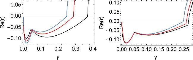
Figure 9. Left panel: the variation of feeding coefficient with real root of a flat-top QD. Blue, red and black curves are drawn for L3 = 0.1, L3 = 0.11 and L3 = 0.125 respectively. For each curve, we take η = 4, g = 0.1, g1 = 0.0005. Right panel: we have drawn the same curves for different values of quantum fluctuation, namely g1 = 0.0005 (blue), g1 = 0.004 (red) and g1 = 0.006(black) respectively at the particular value of L3 = 0.1. |
6. Conclusion
We have studied the dynamics of QDs in BEC both in the absence and presence of three-body recombination. For the case of negligible three-body recombination, we have systematically investigated the properties of sharp- and flat-top quantum droplets using effective potential model. Particularly, we show that the width of a flat-top QD is larger than that of a sharp-top QD for the given value of the number of atoms. We have also studied the time evolution of the width and density profile, and shown that both the width and density profile oscillate with time. However, the amplitude of the oscillation sensitively depends on the initial value of the width around the minimum value of the effective potential.
For a given value of quantum fluctuation, we have shown that the effective width of a droplet increases and the amplitude of its density profile decreases in the presence of three-body loss. The three-body recombination causes the loss of atoms and thus the droplet becomes unstable. Particularly, the width of the density profile of a QD oscillate with the time and the amplitude of the oscillation diminishes as time increases. We have shown that this loss of atoms can, however, be compensated by feeding the droplet from an external source. Thus, it is possible to stabilize the QD for lossless propagation. We also find the stability region using fixed point analysis and show that the stability of a QD depends crucially on the relative strength of three-body loss and external feeding.