


1. Introduction
The transmission of envelope solitons in waveguiding media has been the focus of continuing interest, stimulated by their important potential applications in optical communication systems and optical switching devices [1]. The formation of such wave packets in a monomode optical fiber results from an interplay between nonlinear self-phase modulation and group-velocity dispersion effects [2]. One notes that the experimental observation of solitons has been demonstrated in diverse optical systems, including nonlinear optical fibers [3], glass waveguides [4] and femtosecond ring lasers [5]. Recently, the properties of soliton pulses have been studied extensively due to their important applications for optical transmission and information processing [6].
Usually, the evolution of picosecond light pulses inside a monomode fiber has been more generally governed by the nonlinear Schrödinger equation (NLSE) that is commonly derived with use of the slowly varying envelope approximation [7]. Such a pertinent model has admitted the bright pulse soliton solution in the anomalous dispersion regime while in the normal dispersion region of the fiber it has exhibited the dark-type soliton solution [8]. However, when much shorter optical pulses have to be injected in the fiber, many higher-order dispersive and nonlinear effects have become significant and should have been taken into consideration [9]. For example, the third-order dispersion has considerably influenced the short pulses whose widths are about 50 femtoseconds as they propagate through the nonlinear medium [10, 11]. The quartic dispersion has been also found to be significant when the light pulses are shorter than 10 femtoseconds [10, 11]. In such a case, extensions of the cubic model taking into account the specific contributions of various higher-order effects on the light propagation have been therefore essential to describe the wave dynamics accurately [12]. It has been worth to noting that the occurrence of higher-order processes give rise to a multitude of novel phenomena which are not found in the case of the pure Kerr media [13]. One notes that besides the NLSE and its variants, important results have been also obtained with recent studies discussing diverse nonlinear models which find applications in various sciences and engineering fields, including magnetic fields [14], fluid dynamics [15, 16], magneto-optics [17], quantum mechanics [18], and plasma physics [19]. These models have been used to understand and simulate complex phenomena like solitons in magnetic materials, shallow-water waves in oceans, and the propagation of nonlinear waves in various media. We also note that significant results have been recently obtained by studying the existence and dynamics of various new soliton structures in nonlinear physical systems governed by the NLS-type equations, thus illustrating their significance in fields like optics and Bose–Einstein condensates [20–22]. Techniques like bilinear auto-Bäcklund transformations and similarity reductions have been found to be crucial for finding solutions for such models and understanding system behaviors.
Nowadays, a great interest has been given to the generation of pulse-trains in various physical systems, including birefringent optical fibers [23–27], negative-index materials [28], Bose–Einstein condensates [29], etc. It can be relevant to note that such a type of pulse shape is attracting in itself as another kind of physically relevant nonlinear waves in optical fibers besides the soliton waveforms. These structures exhibit many interesting properties that make them potentially in problems of signal propagation in nonlinear fibers [30]. It is worth mentioning that pulse-trains can be produced experimentally. For example, the formation of cnoidal waves has been recently demonstrated in a fiber laser either in the net anomalous or net normal cavity dispersion regime [31]. Importantly, such pulse-trains may be created from a dual-frequency pump [32] or by the modulational instability of the continuous-wave signal [33]. In optics, such nonlinear structures play a pivotal role in analyzing the data transmission in optical communication links [34].
Recently, a kind of extended NLSE with second-, third-, and fourth-order dispersion terms has been shown to support a stable solitary wave solution with a ${{\rm{{\rm{sech}} }}}^{2}$ shape which is also called quartic soliton [35]. Such kind of stable localized pulses could find practical applications in communications, ultrafast lasers, and slow-light devices [35]. Due to its physical importance in describing femtosecond pulse propagation in highly dispersive optical fibers, such equation has been analyzed from different points of view [35–37]. With regards to the periodic waves, one of the present authors [37] has analytically solved this model and obtained results for periodic wave solutions of the ${{\rm{cn}}}^{2}$ type. However, analytical pulse-train solutions of this extended NLSE that are expressed in terms of products of two different Jacobi elliptic functions have not been reported yet.
Identification of new kinds of pulse-trains in optical systems is an issue worth considering. It is pertinent to mention that the finding of such structures may lead to novel dynamical behaviors of waves and opens the possibility for experimental investigations of various wave phenomena. In this study, we show for the first time that an optical Kerr nonlinear system displaying dispersion effects up to the fourth order supports the existence of three novel classes of pulse-trains which take either single- or double-hump forms The main novelty of these solutions is that the periodic pulse-trains that are composed of products of Jacobian elliptic functions are firstly reported for the extended NLSE with third- and fourth-order dispersions, the interesting amplitude-duration relationship for these structures is found, and the propagation of pulse-train solutions is firstly represented by numerical simulations. In particular, the outcomes presented below constitute the first analytical demonstration of possible pulse-train generation in highly dispersive optical fibers, which may have potential application for the further experiments and research in nonlinear optics. These results will be helpful to nonlinear optics since this kind of nonlinear waves serves as a model of pulse train propagation in optics fibers [34] due to their structural stability with respect to the small input profile perturbations and collisions [38].
The rest of paper is structured as follows. In section 2 , we present the analytic framework necessary to find the traveling wave solutions of the extended NLSE model which governs the transmission of extremely short light pulses through a fiber system depicting higher-order dispersion effects. In section 3 , we derive three different analytic pulse-train solutions of the governing equation and their characteristics. We also discuss here the propagation properties of obtained pulse-trains in the fiber medium. In section 4 , we numerically simulate the propagation of the obtained pulse-train solutions. The stability of the solutions is discussed numerically in section 5 . The conclusions of this paper will be then summarized in section 6 .
2. Model and traveling waves
We consider the propagation of ultrashort light pulses through a nonlinear fiber medium exhibiting the effects of higher-order dispersions as well as self-phase modulation nonlinearity. The governing model for the slowly varying envelope ψ of the light pulse can be described by the extended NLSE [35, 36],
$\begin{eqnarray}{\rm{i}}\frac{\partial \psi }{\partial z}=\alpha \frac{{\partial }^{2}\psi }{\partial {\tau }^{2}}+{\rm{i}}\rm{}\sigma \frac{{\partial }^{3}\psi }{\partial {\tau }^{3}}-\epsilon \frac{{\partial }^{4}\psi }{\partial {\tau }^{4}}-\gamma {\left|\psi \right|}^{2}\psi ,\end{eqnarray}$
where z is the longitudinal coordinate, τ = t − β1z is the retarded time, α = β2/2, σ = β3/6, ε = β4/24, while γ is the fiber nonlinearity coefficient that results in self-phase modulation. Here βj (j = 1, 2, 3, 4) represent, respectively, the dispersion coefficients of the first, second, third, and fourth order.As an important generalization, the extended NLSE (1 ) includes, besides the group-velocity dispersion and self-phase modulation terms that constitute the cubic NLS model, the effects of third- and fourth-order dispersions. These higher-order effects arise in highly dispersive optical systems including dispersion-shifted fibers [39], photonic crystal waveguides (PhCWs) [40], and silicon-based waveguides [41]. It is relevant to note here that the third- and fourth-order dispersions occur in the region of minimum group-velocity dispersion [42], in which they become crucial for describing femtosecond pulse behavior.
Theoretical investigations based on equation (1 ) are mainly concentrated on the existence and propagation properties of localized pulses due to their fundamental importance in the understanding of various physical phenomena in the system. As previously mentioned, Kruglov and Harvey [35] demonstrated the existence of stable solitary waves with a ${{\rm{{\rm{sech}} }}}^{2}$ shape for this model. Triki and Kruglov [36] discussed the dynamics of dipole soliton waveforms of equation (1 ) in the presence the inhomogeneities of media. Kruglov [37] obtained the periodic wave solutions that take the ${{\rm{cn}}}^{2}$ shape for this underlying equation [37]. Cavalcanti et al [42] analyzed the modulation instability of the model (1 ) in the region near the zero-dispersion wavelength. Karpman et al [43, 44] investigated the resonant radiation and evolution of a soliton described by the model (1 ). Shagalov [45] studied the influence of high dispersion terms in the governing equation (1 ) on the modulational instability of nonlinear waves. Roy et al [46] discussed the roles of high-order dispersions in the generation and control of dispersive waves. In what follows, we present three novel analytic pulse-train solutions with interesting properties for the extended NLSE (1 ), which are obtained without necessarily assuming a specified condition on the fiber parameters. Here, the ansatz method which is one of the effective and powerful techniques for finding analytic localized and periodic wave solutions of nonlinear evolution equations [14–16], is used to obtain various types of pulse-trains solutions for the studied model.
In order to find some interesting analytical solutions of the model (1 ), we make the transformation [35, 36],
$\begin{eqnarray}\psi (z,\tau )=\rho (\xi )\exp [{\rm{i}}(\kappa z-\delta \tau +\theta )],\end{eqnarray}$
with ρ(ξ) is the real amplitude and ξ = τ − qz is the traveling coordinate. Here the inverse velocity q = v−1, the frequency shift δ, the wave number κ, and the phase constant θ (at z = 0) are all real parameters to be determined.Inserting equation (2 ) into the extended NLSE (1 ), we get the differential equations: 2 ) with $\rho (\xi )\ne {\rm{constant}}$ as traveling wave or non-plain wave solution.
$\begin{eqnarray}(\sigma +4\epsilon \delta )\frac{{{\rm{d}}}^{3}\rho }{{\rm{d}}{\xi }^{3}}+(q-2\alpha \delta -3\sigma {\delta }^{2}-4\epsilon {\delta }^{3})\frac{{\rm{d}}\rho }{{\rm{d}}\xi }=0,\end{eqnarray}$
$\begin{eqnarray}\begin{array}{l}\epsilon \frac{{{\rm{d}}}^{4}\rho }{{\rm{d}}{\xi }^{4}}-(\alpha +3\sigma \delta +6\epsilon {\delta }^{2})\frac{{{\rm{d}}}^{2}\rho }{{\rm{d}}{\xi }^{2}}\\ +\gamma {\rho }^{3}-(\kappa -\alpha {\delta }^{2}-\sigma {\delta }^{3}-\epsilon {\delta }^{4})\rho =0.\end{array}\end{eqnarray}$
Here, one refers the waveform solution of the model under consideration where the envelope function ψ(z, τ) is defined by the representation (Equations (3 ) and (4 ) with non-zero quartic dispersion coefficient (i.e. ε ≠ 0) give the non-plain wave solutions when the following relations are fulfilled: 3 ) is fulfilled for an arbitrary amplitude function ρ(ξ) in accordance with the conditions in equation (5 ) with ε ≠ 0. Additionally, equation (5 ) allows us to obtain the following expression for the wave velocity v = 1/q,
$\begin{eqnarray}q=2\alpha \delta +3\sigma {\delta }^{2}+4\epsilon {\delta }^{3},\,\,\,\,\delta =-\frac{\sigma }{4\epsilon }.\end{eqnarray}$
Notice that the differential equation ( $\begin{eqnarray}v=\frac{8{\epsilon }^{2}}{\sigma ({\sigma }^{2}-4\alpha \epsilon )}.\end{eqnarray}$
The latter relation shows that the dispersion parameters βi (i = 2, 3, 4) included in the parameters α, σ and ε have a major influence on the wave velocity. This implies that the velocity of the pulse can be efficiently controlled by varying these parameters.
Now using equations (4 ) and (5 ), one can find an equation for ρ as
$\begin{eqnarray}\epsilon \frac{{{\rm{d}}}^{4}\rho }{{\rm{d}}{\xi }^{4}}+b\frac{{{\rm{d}}}^{2}\rho }{{\rm{d}}{\xi }^{2}}-c\rho +\gamma {\rho }^{3}=0,\,\,\,\,\,\,\,\end{eqnarray}$
with $\begin{eqnarray}b=\frac{3{\sigma }^{2}}{8\epsilon }-\alpha ,\,\,\,\,c=\kappa +\frac{{\sigma }^{2}}{16{\epsilon }^{2}}\left(\frac{3{\sigma }^{2}}{16\epsilon }-\alpha \right).\end{eqnarray}$
Equation (7 ) describes the evolution of the wave amplitude in the highly dispersive nonlinear fiber. Now the natural question is whether the amplitude equation (7 ) possesses analytic pulse-train solutions without any specified condition on the coefficients or not. In following, we have identified novel families of pulse-train solutions with some interesting properties for this evolution equation taking into account the influence of all linear and nonlinear processes on pulse propagation.
3. Results and discussion
In this section, we demonstrate that new kinds of pulse-trains can exist in the fiber system governed by equation (1 ). Remarkably, we find that these propagating waves possess distinct amplitudes and consequently different powers, which is highly desired from a practical point of view.
3.1. Pulse-train solutions
Here we show for the first time that equation (7 ) allows for analytic pulse-train solutions which are expressed in terms of the product of different elliptic functions. We find that this type of pulse shape can exist for equation (1 ) in three different classes.
1. Pulse-trains of the ${\rm{cn}}\,\left(x,k\right){\rm{dn}}\,\left(x,k\right)$ -type
We introduce an appropriate ansatz for the propagating waveform solution of equation (7 ) as
$\begin{eqnarray}\rho (\xi )=P\,{\rm{dn}}\left(w(\xi -{\xi }_{0}),k\right){\rm{cn}}\left(w(\xi -{\xi }_{0}),k\right),\end{eqnarray}$
with cosine and the third kind of Jacobian elliptic functions ${\rm{cn}}\left(w(\xi -{\xi }_{0}),k\right)$ and ${\rm{dn}}\left(w(\xi -{\xi }_{0}),k\right)$ of the modulus number k (0 < k < 1). Here P is the amplitude of the wave to be determined and ξ0 is its initial position (at z = 0).Substituting the ansatz (9 ) into equation (7 ) and setting the coefficients of ${{\rm{dn}}}^{j}\left(w(\xi -{\xi }_{0}),k\right){\rm{cn}}\left(w(\xi -{\xi }_{0}),k\right)$ functions (where j = 1, 3, 5) equal to zero, one gets the algebraic equations: 11 ) and (12 ), we get 13 ) into (10 ) yields the parameter c as 8 ) and (14 ), we can obtain the expression for the wave number κ:
$\begin{eqnarray}\epsilon {w}^{4}({k}^{4}-46{k}^{2}+61)-b{w}^{2}({k}^{2}-5)=c,\end{eqnarray}$
$\begin{eqnarray}60\epsilon {w}^{4}{k}^{2}({k}^{2}-3)-6b{w}^{2}{k}^{2}+\gamma ({k}^{2}-1){P}^{2}=0,\end{eqnarray}$
$\begin{eqnarray}120\epsilon {w}^{4}{k}^{2}+\gamma {P}^{2}=0.\end{eqnarray}$
By solving the parametric equations ( $\begin{eqnarray}w=\frac{1}{4}\sqrt{\frac{8\alpha \epsilon -3{\sigma }^{2}}{5{\epsilon }^{2}({k}^{2}+1)}},\,\,\,\,P=\pm \frac{k}{{k}^{2}+1}\sqrt{\frac{-6}{5\gamma \epsilon }}\left(\frac{3{\sigma }^{2}}{8\epsilon }-\alpha \right),\end{eqnarray}$
with γε < 0 and 8αε > 3σ2. Further substitution of equation ( $\begin{eqnarray}c=\frac{(11{k}^{4}-86{k}^{2}+11)}{100\epsilon {({k}^{2}+1)}^{2}}{\left(\frac{3{\sigma }^{2}}{8\epsilon }-\alpha \right)}^{2}.\end{eqnarray}$
Then using equations ( $\begin{eqnarray}\begin{array}{rcl}\kappa & = & \frac{(11{k}^{4}-86{k}^{2}+11)}{100{\epsilon }^{3}{({k}^{2}+1)}^{2}}{\left(\frac{3{\sigma }^{2}}{8}-\alpha \epsilon \right)}^{2}\\ & & -\frac{{\sigma }^{2}}{16{\epsilon }^{3}}\left(\frac{3{\sigma }^{2}}{16}-\alpha \epsilon \right).\end{array}\end{eqnarray}$
Based on these findings, we get a novel periodic wave solution for the model (1 ) as 5 ) and (6 ), respectively.
$\begin{eqnarray}\psi (z,\tau )=P\,{\rm{dn}}\left(w\zeta ,k\right){\rm{cn}}\,\left(w\zeta ,k\right)\exp [{\rm{i}}(\kappa z-\delta \tau +\theta )],\end{eqnarray}$
where ζ = τ − v−1z − ξ0. Note that the frequency shift δ and velocity v of this periodic waveform are defined by the relations (From equation (13 ), one can see that the amplitude P and inverse temporal width w of this periodic wave crucially depend on various dispersion effects as well as nonlinearity. This result indicates that the contributions of dispersions and self-phase modulation processes are essential for this newly found pulse-train to be formed in the optical fiber medium.
We now introduce the quantity τ0 = 1/w which represents the duration of the pulse [47]. Hence, we find that the relation between the pulse amplitude and duration is given by
$\begin{eqnarray}P{\tau }_{0}^{2}=-2k{\left(-{\rm{\Omega }}\right)}^{1/2},\end{eqnarray}$
where the parameter Ω = 30ε/γ has been introduced for brevity. Note that here, we considered the + sign in all the expressions of the wave amplitude.2. Pulse-trains of the ${\rm{cn}}\,\left(x,k\right){\rm{sn}}\,\left(x,k\right)$ -type
We now make an ansatz for equation (7 ) as
$\begin{eqnarray}\rho (\xi )=P\,{\rm{cn}}\,\left(w(\xi -{\xi }_{0}),k\right){\rm{sn}}\,\left(w(\xi -{\xi }_{0}),k\right),\end{eqnarray}$
with cosine and sine Jacobian elliptic functions ${\rm{cn}}\,\left(w(\xi -{\xi }_{0}),k\right)$ and ${\rm{sn}}\,\left(w(\xi -{\xi }_{0}),k\right)$ of the modulus number k (0 < k < 1).Upon substituting of this ansatz into equation (7 ) and then setting the coefficients of $\,{{\rm{cn}}}^{j}\left(w(\xi -{\xi }_{0}),k\right){\rm{sn}}\left(w(\xi -{\xi }_{0}),k\right)$ functions (where j = 1, 3, 5) equal to zero, we obtain the algebraic equations: 19 ) and (22 ), we have the expression:
$\begin{eqnarray}\epsilon {w}^{4}(61{k}^{4}-76{k}^{2}+16)+b{w}^{2}(5{k}^{2}-4)=c,\end{eqnarray}$
$\begin{eqnarray}60\epsilon {w}^{4}{k}^{2}(3{k}^{2}-2)+6b{w}^{2}{k}^{2}+\gamma {P}^{2}=0,\end{eqnarray}$
$\begin{eqnarray}120\epsilon {\eta }^{4}{k}^{2}-\gamma {P}^{2}=0.\end{eqnarray}$
Based on these equations, one obtains the relations for the inverse width w of the wave and its amplitude P as $\begin{eqnarray}\begin{array}{rcl}w & = & \frac{1}{4}\sqrt{\frac{3{\sigma }^{2}-8\alpha \epsilon }{5{\epsilon }^{2}(4-3{k}^{2})}},\\ P & = & \pm \frac{k}{4-3{k}^{2}}\sqrt{\frac{6}{5\gamma \epsilon }}\left(\frac{3{\sigma }^{2}}{8\epsilon }-\alpha \right),\end{array}\end{eqnarray}$
with γε > 0 and 3σ2 > 8αε. Additionally, by using equations ( $\begin{eqnarray}c=\frac{{b}^{2}(244{k}^{2}-89{k}^{4}-144)}{100\epsilon {(4-3{k}^{2})}^{2}}.\end{eqnarray}$
Then from equations (8 ) and (23 ), we find that the wave number κ of the periodic wave solution takes the form as 1 ) as 5 ) and (6 ), respectively.
$\begin{eqnarray}\begin{array}{rcl}\kappa & = & \frac{(244{k}^{2}-89{k}^{4}-144)}{100{\epsilon }^{3}{(4-3{k}^{2})}^{2}}{\left(\frac{3{\sigma }^{2}}{8}-\alpha \epsilon \right)}^{2}\\ & & -\frac{{\sigma }^{2}}{16{\epsilon }^{3}}\left(\frac{3{\sigma }^{2}}{16}-\alpha \epsilon \right).\end{array}\end{eqnarray}$
These results yield a new kind of pulse-train solution for the NLSE model ( $\begin{eqnarray}\psi (z,\tau )=P\,{\rm{cn}}\,\left(w\zeta ,k\right){\rm{sn}}\,\left(w\zeta ,k\right)\exp [{\rm{i}}(\kappa z-\delta \tau +\theta )],\end{eqnarray}$
where ξ = τ − v−1z − ξ0. Noting that the frequency shift δ and velocity v in this periodic structure are defined by the relations (For this solution, we find that the relation between the pulse amplitude and duration takes the form,
$\begin{eqnarray}P{\tau }_{0}^{2}=2k{\left({\rm{\Omega }}\right)}^{1/2}.\end{eqnarray}$
3. Pulse-trains of the ${\rm{dn}}\left(x,k\right){\rm{sn}}\left(x,k\right)$ -type
Next we make an ansatz for equation (7 ) as
$\begin{eqnarray}\rho (\xi )=P\,{\rm{dn}}\left(w(\xi -{\xi }_{0}),k\right){\rm{sn}}\left(w(\xi -{\xi }_{0}),k\right).\end{eqnarray}$
Substituting this ansatz into the amplitude equation (7 ) and then setting the coefficients of $\,{{\rm{dn}}}^{j}\left(w(\xi -{\xi }_{0}),k\right){\rm{sn}}\left(w(\xi -{\xi }_{0}),k\right)$ functions (where j = 1, 3, 5) equal to zero, one finds the algebraic equations:
$\begin{eqnarray}\epsilon {w}^{4}(16{k}^{4}-76{k}^{2}+61)+b{w}^{2}(5{k}^{2}-4)=c,\end{eqnarray}$
$\begin{eqnarray}60\epsilon {w}^{4}{k}^{2}(2{k}^{2}-3)-6b{w}^{2}{k}^{2}+\gamma {P}^{2}=0,\end{eqnarray}$
$\begin{eqnarray}120\epsilon {w}^{4}{k}^{2}-\gamma {P}^{2}=0.\end{eqnarray}$
Solving these equations, one can get the pulse parameters w and P as $\begin{eqnarray}\begin{array}{rcl}w & = & \frac{1}{4}\sqrt{\frac{3{\sigma }^{2}-8\alpha \epsilon }{5{\epsilon }^{2}(2{k}^{2}-1)}},\\ P & = & \pm \frac{k}{2{k}^{2}-1}\sqrt{\frac{6}{5\gamma \epsilon }}\left(\frac{3{\sigma }^{2}}{8\epsilon }-\alpha \right),\end{array}\end{eqnarray}$
with γε > 0 and 8αε < 3σ2 when $1/\sqrt{2}\lt k\lt 1$ and 8αε > 3σ2 when $0\lt k\lt 1/\sqrt{2}$.Moreover, the use of equations (28 ) and (31 ) lead to an expression for the parameter c as
$\begin{eqnarray}c=\frac{{b}^{2}(64{k}^{2}-64{k}^{4}+11)}{100\epsilon {(2{k}^{2}-1)}^{2}}.\end{eqnarray}$
Now using equations (8 ) and (32 ), we can determine the wave number κ as 1 ) as 5 ) and (6 ), respectively.
$\begin{eqnarray}\begin{array}{c}\kappa \,=\,\frac{(64{k}^{2}-64{k}^{4}+11)}{100{\epsilon }^{3}{(2{k}^{2}-1)}^{2}}{\left(\frac{3{\sigma }^{2}}{8}-\alpha \epsilon \right)}^{2}-\frac{{\sigma }^{2}}{16{\epsilon }^{3}}\left(\frac{3{\sigma }^{2}}{16}-\alpha \epsilon \right).\end{array}\end{eqnarray}$
Thus, we find a novel pulse-train solution for the NLSE model ( $\begin{eqnarray}\psi (z,\tau )=P\,{\rm{dn}}\left(w\zeta ,k\right){\rm{sn}}\left(w\zeta ,k\right)\exp [{\rm{i}}(\kappa z-\delta \tau +\theta )],\end{eqnarray}$
where ξ = τ − v−1z − ξ0. Here δ and v can be worked out by using the relations (For this solution, we find that the relation between the pulse amplitude and duration takes the form,
$\begin{eqnarray}P{\tau }_{0}^{2}=2k{\left({\rm{\Omega }}\right)}^{1/2}.\end{eqnarray}$
On comparing equations (17 ), (26 ) and (35 ), we infer that under the effects of quadratic, cubic and quartic dispersions and self-phase modulation nonlinearity, the fiber system allows the propagation of distinct types of pulse-trains which present a relation between the pulse amplitude and duration determined by the sign of the joint parameter Ω = 30ε/γ only. To our knowledge, the pulse-trains derived above for equation (1 ) are firstly presented in this work.
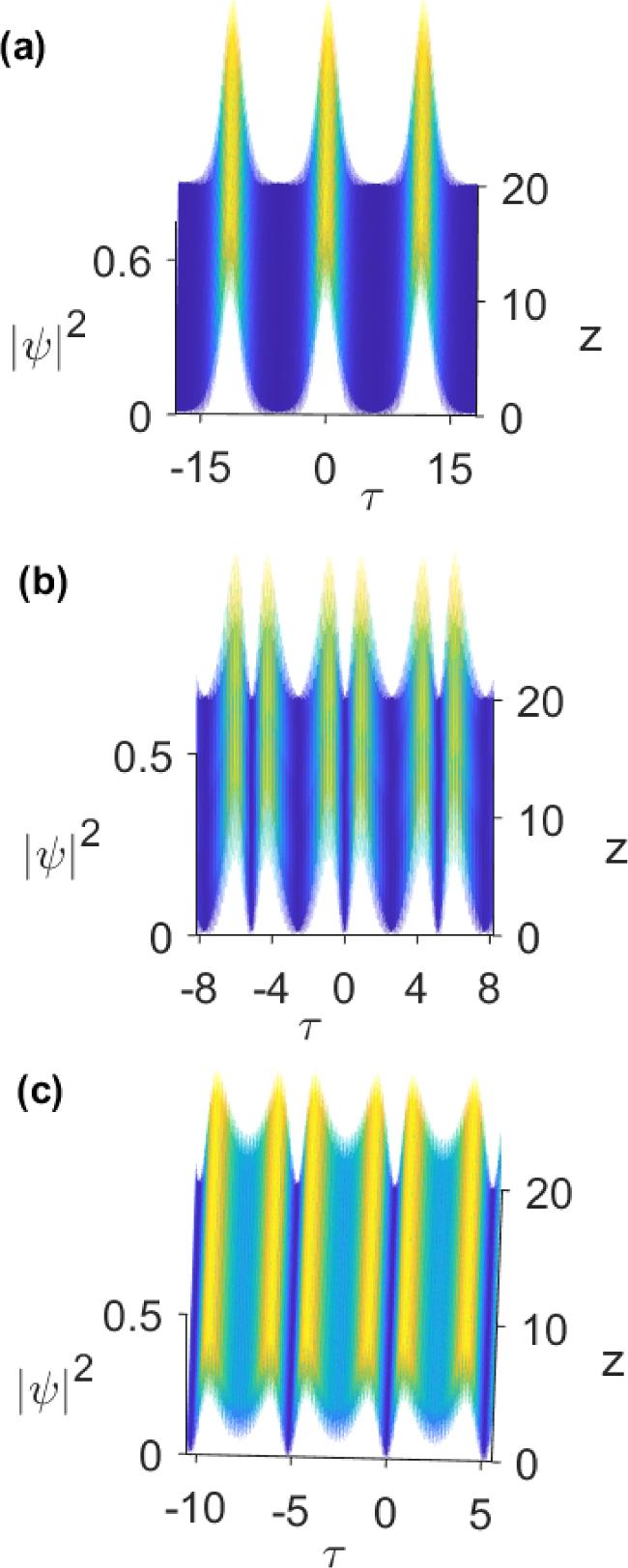
Figure 1(a) depicts the intensity profile of the pulse-train solution (16 ) of the model (1 ) for the parameters values: α = −1, γ = 2, σ = −0.25, and ε = −0.25. The results for the pulse-train solutions (25 ) and (34 ) are shown in figures 1(b) and (c) for the values α = 0.49, γ = 2, σ = 1, and ε = 0.5. One notes here that the value of initial position ξ0 (at z = 0) of the nonlinear waves is chosen zero. Also, the modulus number k is selected to be k = 0.9. The evolution of these pulse-train solutions in the fiber medium are displayed in figure 2. From these figures, we observe that the three types of pulse-train solutions are positive and exhibit an oscillating behavior. In addition, we can see that the pulse-train solutions (25 ) and (34 ) present two peaks in each periodic unit, markedly different from the pulse train solution (16 ) which has a one peak structure.
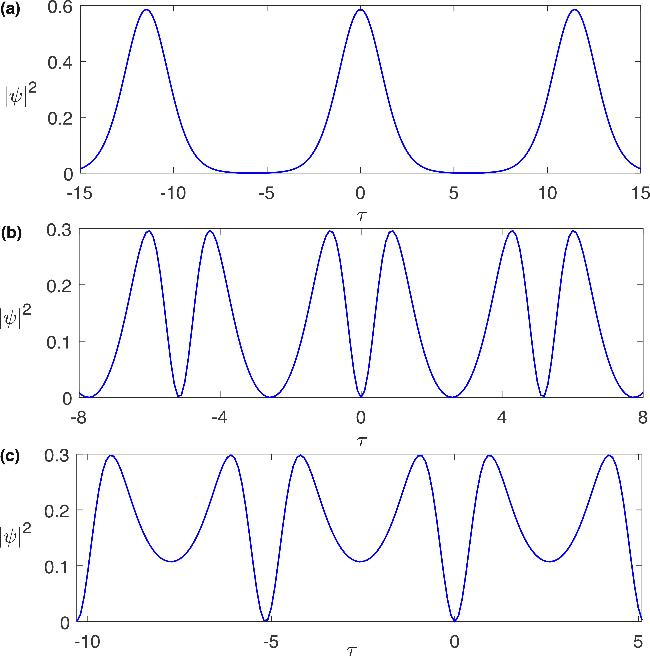
Figure 1. Intensity profiles of pulse-train solutions with parameters γ = 2, k = 0.9, ξ0 = 0; (a) pulse-train solution ( |
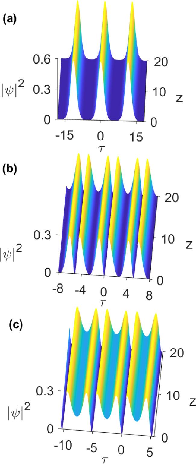
Figure 2. Intensity profiles of pulse-train solutions with parameter k = 0.9; (a) pulse-train solution ( |
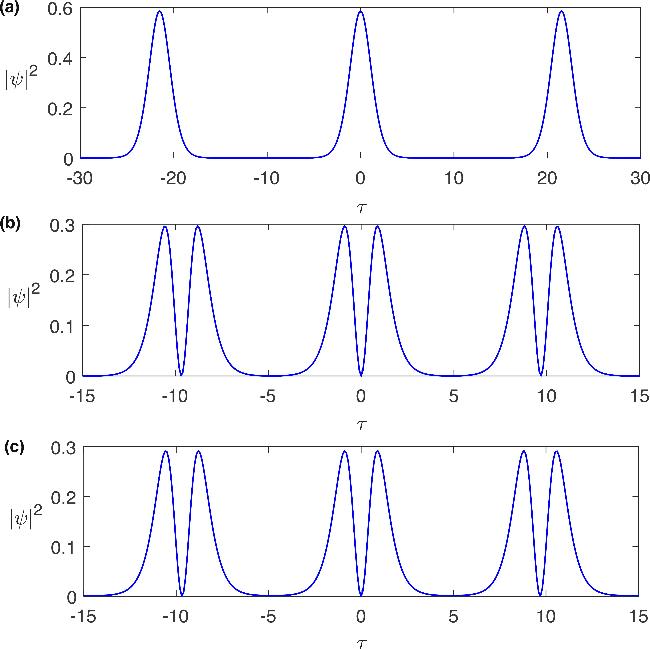
Figure 3. Evolution of pulse-train solutions with parameter k = 0.999; (a) pulse-train solution ( |
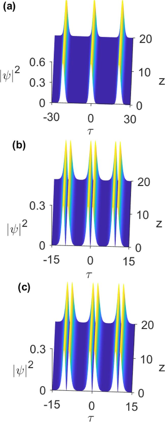
Figure 4. Evolution of pulse-train solutions with parameter k = 0.999; (a) pulse-train solution ( |
A key observation is that the amplitudes, widths and wave numbers of the derived pulse-train solutions are different whereas their velocity is the same. More importantly, the expression (6 ) demonstrates that the velocity of these pulse-trains can be considerably diminished for suitable parameters of the waveguiding media, which have application value in the development of slow-light systems. Recently, Li and Huang [48] studied the modification of a slow-light soliton in three-level atomic systems. They derived a high-order NLSE incorporating third-order dispersion, delay in nonlinear refractive index, modulation induced by the microwave field, nonlinear dispersion, and correction terms of linear and differential absorptions; and demonstrated that an obvious decrease of propagating velocity of the soliton can be obtained in the presence of the microwave field. Note that PhCWs represent interesting slow light structures due to their confinement and versatile dispersion properties including slow light and possible control of group velocity dispersion effects [49–51]. In order to strictly answer the question of possibility of applying the newly found pulse-trains in the development of slow-light systems much further research is needed. A detailed investigation of this problem will be reported in a forthcoming publication.
In figure 5, we present the dependence of velocity on the group velocity dispersion parameter α of the medium for three distinct values of quartic dispersion coefficient ε. We clearly see that the wave velocity decreases intensely in the magnitude as the value of dispersion parameter α is increased. The decrease of velocity implies that the slowing motion of pulse-trains is possible in the transmitting medium when considering large dispersion parameter α. It is also observed that the pulse velocity has large magnitude for small negative values of ε. Hence, one concludes that the velocity of pulse-trains can be controlled by judicious choice of the dispersion coefficients.
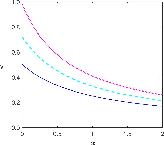
Figure 5. Dependence of the velocity of pulse-trains v on the group velocity dispersion parameter α for σ = 1 and different values of ε; ε = −0.25 (thick line), ε = −0.3 (dashed line) and ε = −0.35 (dotted line). |
3.2. Quartic and dipole soliton solutions
We now focus on the long-wave limit of the new pulse-trains obtained above corresponding to the modulus k = 1. In such a case, the periodic solution (16 ) degenerates to the quartic soliton solution [35]: 5 ) and the velocity v is defined by equation (6 ).
$\begin{eqnarray}\begin{array}{rcl}\psi (z,\tau ) & = & {P}_{0}\,{{\rm{{\rm{sech}} }}}^{2}\left[{w}_{0}\left(\tau -{v}^{-1}z-{\xi }_{0}\right)\right]\\ & & \times \exp [{\rm{i}}(\kappa z-\delta \tau +\theta )],\end{array}\end{eqnarray}$
where the inverse temporal width w0, amplitude P0 and wave number κ of the soliton pulse are given by $\begin{eqnarray}{w}_{0}=\frac{1}{4}\sqrt{\frac{8\alpha \epsilon -3{\sigma }^{2}}{10{\epsilon }^{2}}},\end{eqnarray}$
$\begin{eqnarray}{P}_{0}=\pm \sqrt{\frac{-3}{10\gamma \epsilon }}\left(\frac{3{\sigma }^{2}}{8\epsilon }-\alpha \right),\end{eqnarray}$
$\begin{eqnarray}\kappa =-\frac{4}{25{\epsilon }^{3}}{\left(\frac{3{\sigma }^{2}}{8}-\alpha \epsilon \right)}^{2}-\frac{{\sigma }^{2}}{16{\epsilon }^{3}}\left(\frac{3{\sigma }^{2}}{16}-\alpha \epsilon \right),\end{eqnarray}$
with γε < 0 and 8αε > 3σ2. Here the soliton frequency shift δ is given by equation (Notice that for this quartic soliton waveform, the relation between the amplitude and duration is given by
$\begin{eqnarray}{P}_{0}{\tau }_{0}^{2}=-2\sqrt{\frac{-30\epsilon }{\gamma }},\end{eqnarray}$
provided that γε < 0.In addition, when k → 1, the periodic solution (25 ) transforms into our dipole soliton solution [36]: 5 ) and its velocity v is defined by equation (6 ).
$\begin{eqnarray}\begin{array}{rcl}\psi (z,\tau ) & = & {P}_{0}\,{\rm{{\rm{sech}} }}\left[{w}_{0}\left(\tau -{v}^{-1}z-{\xi }_{0}\right)\right]{\rm{th}}\left[{w}_{0}\left(\tau -{v}^{-1}z-{\xi }_{0}\right)\right]\\ & & \times \,\exp [{\rm{i}}(\kappa z-\delta \tau +\theta )],\end{array}\end{eqnarray}$
where the inverse temporal width w0, amplitude P0 and wave number κ of the soliton pulse take the form, $\begin{eqnarray}{w}_{0}=\frac{1}{4}\sqrt{\frac{3{\sigma }^{2}-8\alpha \epsilon }{5{\epsilon }^{2}}},\end{eqnarray}$
$\begin{eqnarray}{P}_{0}=\pm \sqrt{\frac{6}{5\gamma \epsilon }}\left(\frac{3{\sigma }^{2}}{8\epsilon }-\alpha \right),\end{eqnarray}$
$\begin{eqnarray}\kappa =\frac{11}{100{\epsilon }^{3}}{\left(\frac{3{\sigma }^{2}}{8}-\alpha \epsilon \right)}^{2}-\frac{{\sigma }^{2}}{16{\epsilon }^{3}}\left(\frac{3{\sigma }^{2}}{16}-\alpha \epsilon \right),\end{eqnarray}$
with γε > 0 and 8αε < 3σ2. Notice that the frequency shift δ of this dipole soliton is given by equation (It is interesting to note that if one considers the limiting case with k = 1, the pulse-train solution (34 ) also becomes the same dipole-type soliton solution (41 ). Notice that for this kind of solitons, we obtain a relation between the pulse amplitude and duration as:
$\begin{eqnarray}{P}_{0}{\tau }_{0}^{2}=2\sqrt{\frac{30\epsilon }{\gamma }},\end{eqnarray}$
provided that γε > 0.4. Propagation of pulse-trains in extended NLSE with higher-order dispersion
For completeness, we have numerically simulated the propagation of pulse-train solutions (16 ), (25 ) and (34 ) in equation (1 ) by utilizing the split-step Fourier method [52]. The physical parameters used in this model for the case of pulse-train solution (16 ) are representative of a femtosecond Ti:sapphire laser [53]: β2 = −100 fs2 cm−1, β3 = −500 fs3 cm−1, β4 =−5000 fs4 cm−1, and γ = 2.36 × 10⁻⁶ W−1 cm−1. Note that these experimental parameters satisfy the relations γε < 0 and 8αε > 3σ2 which are necessary and sufficient for the existence of the pulse-train solution (16 ). As concerns the pulse-train solutions (25 ) and (34 ), we use the parameters of the silicon-based slot waveguide as [36, 41]: β2 = −0.05 ps2 m−1, β3 = 1.9 × 10⁻⁵ ps3 m−1, β4 = 2.5 × 10⁻⁵ ps4 m−1, and γ = 42 W−1 cm−1. We point out that with these system parameters, the relations γε > 0 and 8αε < 3σ2 for the existence of pulse-train solutions (25 ) and (34 ) are fulfilled. Figure 6 illustrates the evolutions of periodic pulse-trains propagating through a distance of 20 dispersion lengths. Here the elliptic modulus is chosen as k = 0.9. We can see that the pulse-train solutions (16 ), (25 ) and (34 ) can preserve their shape during propagation due to the balance between the effects of quadratic, cubic and quartic dispersions and the Kerr nonlinearity in the system.
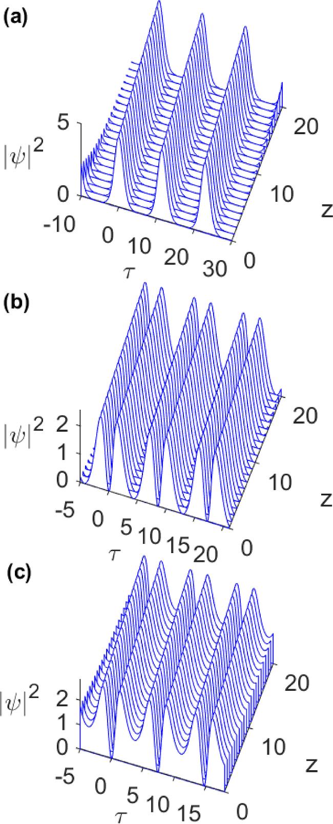
Figure 6. Evolution of the intensity distribution of the extended NLSE; (a) pulse-train solution ( |
Finally, the figures presented above indicate that the newly found pulse-train solutions have no oscillated tails on the wings of pulses. It is important to mention that experimental and numerical studies have demonstrated that solitons propagating in nonlinear Kerr media with dominant fourth-order dispersion are approximately Gaussian with oscillating tails [54, 55]. By considering the influence of both second-, third- and fourth-order dispersions on the pulse propagation through fibers, one of the present authors has recently obtained quartic solitons with a ${{\rm{{\rm{sech}} }}}^{2}$ shape which does not carry oscillating tails [35]. Under these conditions, we have also found that dipole solitons without oscillating tails are formed in the highly dispersive fiber system [36]. These important results show that dispersive effects up to the fourth order and Kerr nonlinearity can achieve a perfect balance under certain conditions and lead to the formation of solitons without oscillating tails. No doubt, the pulse-trains presented here may be of guidance for the experimental generation of optical periodic waves due to their precise nature and interesting amplitude-duration relationship.
5. Stability of the pulse-train solutions
To complete the discussion of the pulse-train solutions found above, we study their stability with respect to the finite perturbations numerically. It is crucially important to note that only solutions that are stable (or weakly unstable) can be observed in physical experiments and used in practical applications [56]. We mention in passing that quartic and dipole soliton solutions to the extended NLSE (1 ) are found to be stable with respect to finite perturbations [35, 36]. Here we perform direct numerical simulations of the model (1 ) using the split-step Fourier method [52], to test the stability of pulse-train solutions (16 ), (25 ) and (34 ) with initial white noise, as compared to figures 2(a)–(c), respectively. As usual, we put the noise onto the initial profile, then the perturbed pulses read [57]: ψpert = ψ(τ, 0)[1 + 0.1 random(τ)]. Figures 7(a)–(c) depict the numerical evolution of nonlinear wave solutions under the perturbation of white noise. From these figures, we can see that the pulse-train waveforms can propagate in a stable way under the initial perturbation of white noise. Thus, we can conclude that the solutions we obtained are stable.
Figure 7. The numerical evolution; (a) pulse-train solution ( |
6. Conclusion
In conclusion, we have discovered three classes of pulse-trains whose amplitudes, widths and wavenumbers are different with the distinctive property of exhibiting a relation between the amplitude and duration determined by the sign of a joint parameter uniquely. We have found that these structures have the same velocity, which depends only on the three dispersion parameters. It is demonstrated that higher-order dispersion may lead to the formation of double-humped pulse-trains besides the ones taking the usual form with single peak in each periodic unit. It is also shown that the pulse-trains are obtained without necessarily assuming a specified condition on the fiber parameters. Due to the precise nature, the nonlinear waves presented here may be profitably used in designing the optimal fiber system experiments. These results can be exploited to experimentally realize pulse-trains in fiber systems and may help in stimulating more research in understanding their optical transmission properties.