


Introduction
Voting is an essential mechanism of modern democratic life for expressing public opinion [1]. The intent of voting is for the outcome to reflect the will of the majority of participants, but in the information era, media and social platforms may potentially influence or even manipulate voting results through opinion guidance [2, 3]. It is therefore necessary to quantitatively study the impact of real-time information on voting outcomes with the aid of statistical physics [4–6]. In this study, we consider a form of ‘fair' real-time information feedback, where the media provides unbiased information: voters are allowed to know the current overall voting trend in real time and make their next voting decisions based on this information.
To derive general conclusions, we have to introduce a highly simplified statistical model. We consider only binary voting decisions, where each agent can vote either ‘yes' or ‘no'. The Ising model is well-suited for simulating such scenarios. In the Ising model, each site (representing a voter) has a spin variable that can be +1 (spin up, representing a ‘yes' vote) or –1 (spin down, representing a ‘no' vote). Each agent is influenced by its nearest neighbors ($z=2d$ neighbors in a d-dimensional model), tending to align its vote with those neighbors. The Hamiltonian (energy function) of the conventional Ising model without external fields [7] is
$\begin{eqnarray}H=-{J}_{0}\displaystyle \displaystyle \sum _{\left\langle i,j\right\rangle }{s}_{i}{s}_{j},\end{eqnarray}$
where ${s}_{i}=\pm 1$ is the spin (vote) of agent $i$, the sum runs over all pairs of neighboring sites $\left\langle i,j\right\rangle $, and the constant ${J}_{0}\gt 0$ is the interaction strength favoring the alignment of neighboring spins. The periodic boundary condition is applied, so the last and first spins in one dimension are a pair of neighbors. The system temperature $T$ is a relative concept compared to the interaction strength: a higher temperature corresponds to weaker effective influence of neighbors, meaning that voters make more independent decisions (higher ‘autonomy'), whereas a lower temperature means neighbors have a stronger influence (voters are more conformist). The total magnetization $M=\displaystyle {\sum }_{i=1}^{N}{s}_{i}$ represents the net vote count (difference between ‘yes' and ‘no' votes) and N is the number of sites (voters).The conventional Ising model is a well-studied paradigm of phase transitions in statistical physics. In one dimension (a linear chain of spins), the Ising model does not exhibit a phase transition at finite temperatures—thermal fluctuations are strong enough to prevent any long-range order [8]. In other words, for the 1D Ising model, the ensemble-averaged magnetization $\left\langle M\right\rangle =0$ remains zero for any $T\gt 0$, indicating that, without external influences, the numbers of ‘yes' and ‘no' votes tend to balance out. By contrast, in two and higher dimensions, the Ising model undergoes a second-order phase transition at a critical temperature ${T}_{{\rm{c}}}$. Above ${T}_{{\rm{c}}}$, the system is disordered: thermal fluctuations dominate, and the average magnetization is zero (no overall majority). Below ${T}_{{\rm{c}}}$, the system becomes ordered: the interactions dominate over thermal noise, leading to a spontaneous magnetization (a majority of ‘yes' or ‘no' votes). The critical temperature marks the onset of a collective behavior where the population can polarize into a majority opinion when the dimension $d\gt 1$, but not when $d=1$.
We are now interested in the question: How does real-time knowledge of the overall voting trend affect the outcome? To investigate this problem, we modify the conventional Ising model to include positive feedback in the interaction between neighbors. In our intelligent Ising model, the interaction strength between neighbors is not a constant anymore; instead, it increases with the instantaneous total magnetization, creating a positive feedback loop. This mimics a scenario where voters, seeing a growing strength of majority, feel increased pressure to conform with their neighbors. The Hamiltonian for the intelligent Ising model can be written as
$\begin{eqnarray}H=-J\left(m\right)\displaystyle \sum _{\left\langle i,j\right\rangle }{s}_{i}{s}_{j},\end{eqnarray}$
where the interaction becomes a function of the specific magnetization $m\equiv M/N$: $\begin{eqnarray}J\left(m\right)={J}_{0}\left(1+k{m}^{2}\right),\end{eqnarray}$
with $k$ the coupling strength between $J$ and $m$. Since the coupling $J\left(m\right)$ depends on the specific magnetization $m=M/N$, which is an intensive variable, the total energy is still an extensive variable and scales as $H\unicode{x0007E}O\left(N\right)$. As a result, the free energy density $F/N$ converges in the thermodynamic limit, and the existence of a stable thermal equilibrium state is ensured. The Boltzmann distribution is therefore applicable.The concept of the intelligent Ising model draws inspiration from recent advances in soft matter physics [9]. Soft materials (such as polymers, liquid crystals, colloids, and biological matter) owe their ‘softness' to a delicate balance to the free energy landscape between enthalpic and entropic contributions [10]. Building on this, the field of active matter has emerged to describe systems of many self-driven units [11, 12] (e.g. bacterial swarms, bird flocks, fish schools) that consume energy to move or make decisions. Active matter systems can exhibit collective behaviors (like flocking or swarming) [13, 14] that are not seen in equilibrium systems, due to the continuous input of energy at the individual level. However, traditional active matter models do not explicitly include adaptive feedback in interactions [15]. We propose that an essential feature of intelligent agents (such as human voters [16, 17] or animals with learning) is the ability to adaptively adjust interactions in response to dynamic conditions via feedback mechanisms [18–20]. In other words, unlike passive particles or simple self-propelled agents, intelligent agents can change how strongly they influence or are influenced by others based on input information. From the viewpoint of statistical mechanics, a group of intelligent agents can be named as intelligent matter, which can be used to model and study a collective of behaving individuals with intelligence. This is precisely what our intelligent Ising model implements: the interaction strength adapts in response to the global magnetization (the current vote tally).
In this work, we study the phase behaviors of the intelligent Ising model using both analytical derivations and computer simulations. Our findings reveal striking differences from the conventional model due to the feedback mechanism: a phase transition occurs even in one dimension as the temperature is varied, and a small imbalance can grow and lock in due to the increasing coupling, leading to a spontaneous magnetization at low temperatures; a second-order phase transition exhibits at a weaker coupling strength $k$ and a first-order phase transition at a stronger $k$; a special point called the tricritical point [8] marking the boundary where the transition changes its order from second to first. This rich phase behavior arises purely from the feedback-induced adaptation of interactions. Translating these results back to the voting scenario, we demonstrate that real-time information about collective opinion can significantly alter voting dynamics. Even unbiased feedback may possibly induce spontaneous symmetry-breaking, leading to a biased outcome where one side of the vote becomes favored.
Results
Analytic solution of the 1D intelligent Ising model
To analyze the phase behavior of the model, we utilize the parameterized free energy2 ) is7 ), this model has an exact analytical solution. As detailed in the Methods section, we obtain the exact analytical solution of the free energy density at the thermodynamic limit
$\begin{eqnarray}F\left(m\right)=-\displaystyle \frac{1}{\beta }\,{\mathrm{ln}}\,{Z}_{N}\left(m\right),\end{eqnarray}$
where $\beta \equiv \displaystyle \frac{1}{{k}_{{\rm{B}}}T}$ with ${k}_{{\rm{B}}}$ the Boltzmann constant, and the partition function corresponding to equation ( $\begin{eqnarray}{Z}_{N}\left(m\right)=\displaystyle \displaystyle \sum _{\left\{{s}_{i}\right\}}\delta \left(\displaystyle \frac{1}{N}\displaystyle \sum _{i=1}^{N}{s}_{i}-m\right)\exp \left(\beta J\left(m\right)\displaystyle \sum _{i=1}^{N}{s}_{i}{s}_{i+1}\right).\end{eqnarray}$
In one dimension, similar to the conventional Ising model ( $\begin{eqnarray}\begin{array}{rcl}f\left(m\right)\equiv F\left(m\right)/N & = & -\displaystyle \frac{1}{\beta }\,{\mathrm{ln}}\left[\sqrt{{{\rm{e}}}^{2\beta J\left(m\right)}+{{\rm{e}}}^{-2\beta J\left(m\right)}\displaystyle \frac{{m}^{2}}{1-{m}^{2}}}\right.\\ & & \left.+\,\displaystyle \frac{{{\rm{e}}}^{-\beta J\left(m\right)}}{\sqrt{1-{m}^{2}}}\right]\\ & & +\,\displaystyle \frac{m}{\beta }\,{\mathrm{ln}}\left[{{\rm{e}}}^{-2\beta J\left(m\right)}\displaystyle \frac{m}{\sqrt{1-{m}^{2}}}\right.\\ & & \left.+\,\sqrt{1+{{\rm{e}}}^{-4\beta J\left(m\right)}\displaystyle \frac{{m}^{2}}{1-{m}^{2}}}\right].\end{array}\end{eqnarray}$
This expression characterizes the thermodynamic behavior of the system by the fact that its minima corresponding to stable or metastable phases, and its phase behavior is determined by the feedback strength $k$ and the temperature $T$.The exact analytical solution of the 1D intelligent Ising model reveals rich phase behavior modulated by the coupling strength k. The phase diagram, as shown in figure 1(a), is plotted in the $\left(k,{T}^{* }\right)$ plane, where the dimensionless temperature ${T}^{* }={k}_{{\rm{B}}}T/{J}_{0}$. The white region corresponds to the paramagnetic phase characterized by $\left\langle m\right\rangle =0$, while the blue region represents the ferromagnetic phase with spontaneous magnetization where $\left\langle m\right\rangle \ne 0$. The dashed curve marks the spinodal line, beyond which the metastable states vanish.
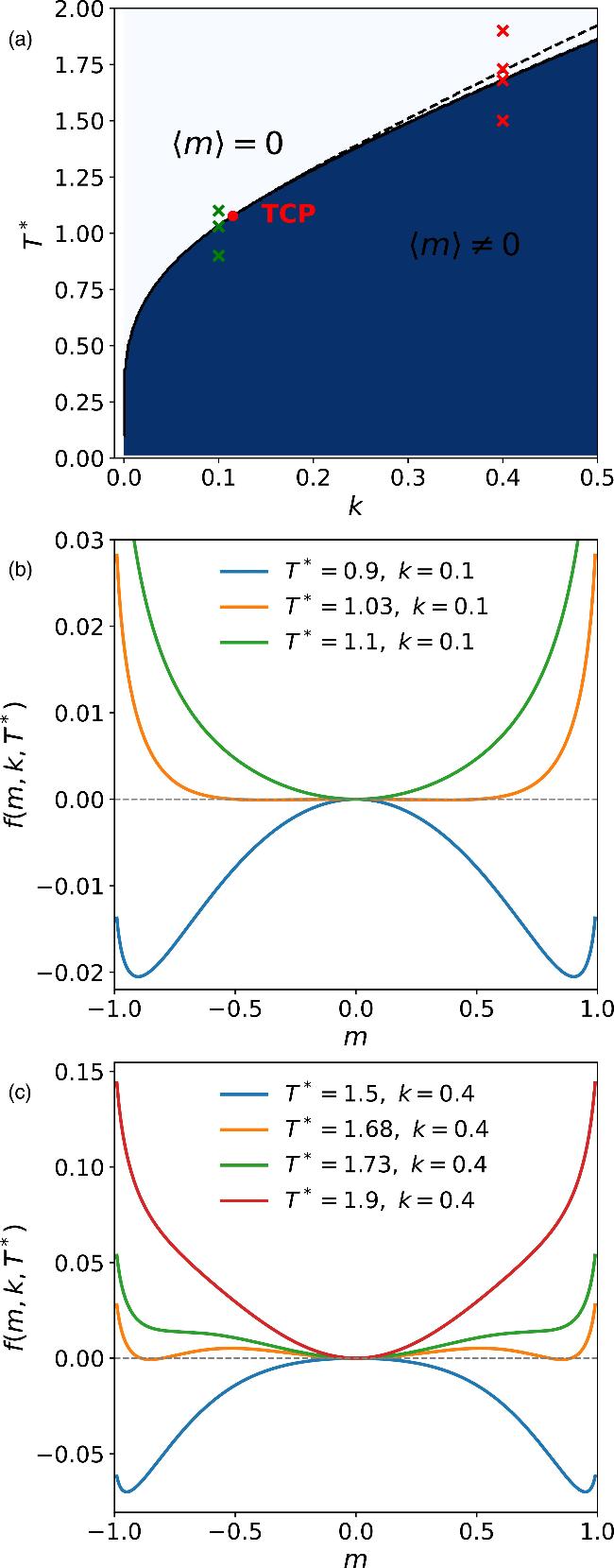
Figure 1. (a) Phase diagram derived from the exact analytical solution of the 1D intelligent Ising model in the $(k,{T}^{* })$ space. The white and blue regions correspond to the paramagnetic phase ($\langle m\rangle =0$) and the ferromagnetic phase ($\langle m\rangle \ne 0$), respectively. The dashed line denotes the spinodal line obtained from the stability condition ${\partial }^{2}f/\partial {m}^{2}=0$ of the exact free-energy landscape. The red dot marks the tricritical point determined from the Landau expansion of the exact free-energy landscape. (b) Exact free-energy landscape $f(m,k,{T}^{* })$ for $k=0.1$ at representative temperatures (green crosses in panel (a)), showing a continuous phase transition. (c) Exact free-energy landscape $f(m,k,{T}^{* })$ for $k=0.4$ at representative temperatures (red crosses in panel (a)), showing a discontinuous phase transition. |
From the phase diagram, we observe that at k = 0, the critical temperature Tc approaches zero, consistent with the well-known result of the conventional 1D Ising model. As k increases from zero, Tc rises sharply, indicating that even a small nonlinear feedback strength k can induce a finite-temperature phase transition in the 1D Ising model. For larger k, the growth of Tc continues but becomes more gradual.
Interestingly, the nature of the phase transition also changes with $k$. For $k\lt {k}_{{\rm{c}}}$, the phase transition from low to high temperature is continuous (second-order). By contrast, for $k\gt {k}_{{\rm{c}}}$, the phase transition becomes discontinuous [21] (first-order) with hysteresis. This change in transition order is clearly reflected in the free energy landscapes: as shown in figure 1(b), for k = 0.1, the minimum of the free energy landscape evolves continuously with temperature, indicating a continuous phase transition; while for k = 0.4, figure 1(c) reveals the emergence of competing minima separated by a barrier, signaling metastability and phase coexistence. These features suggest the presence of a tricritical point on the phase boundary where the transition shifts from second to first order.
To accurately locate the tricritical point, we perform a Landau expansion of the free energy up to the sixth-order term in the order parameter [8] as
$\begin{eqnarray}\begin{array}{rcl}f\left(m;k,T\right) & = & {f}_{0}+a\left(k,T\right){m}^{2}+b\left(k,T\right){m}^{4}\\ & & +\,c\left(k,T\right){m}^{6}+O\left({m}^{7}\right).\end{array}\end{eqnarray}$
When $a\left(k,T\right)=b\left(k,T\right)=0$ and $c\left(k,T\right)\gt 0$, the system is at the tricritical point with ${k}_{{\rm{c}}}=0.1115$ and ${T}_{{\rm{c}}}=1.077$. This point marks the boundary between the continuous (second-order) and discontinuous (first-order) phase transitions, indicating a fundamental change in the nature of the phase transition.Simulation results for the 1D intelligent Ising model
To validate the analytical predictions, we employ the Metropolis Monte Carlo (MC) algorithm [22] to simulate the evolution of the spin configurations in the 1D intelligent Ising model at various values of k. For each k, a pseudo-critical temperature ${T}_{{\rm{c}}}(k)$ is identified from the peak position of the specific heat ${C}_{V}(T)$ for a finite system. As shown in figure 2(a), the resulting ${T}_{{\rm{c}}}(k)$ defines a pseudo-critical line, along which further analysis is carried out. As shown in figure 2(b), the peak of ${C}_{V}(T)$ becomes progressively sharper with increasing k, indicating enhanced energy fluctuations near the transition. The corresponding energy probability distributions $P(E)$ evaluated at $(k,{T}_{{\rm{c}}}(k))$ are used to extract the energy separation ${\rm{\Delta }}{E}_{{\rm{sep}}}$ between coexisting states when a double-peak structure is present. For a small k, $P(E)$ exhibits a single peak and ${\rm{\Delta }}{E}_{{\rm{sep}}}=0$, consistent with a continuous transition. By contrast, for a sufficiently large k, a clear double-peak structure emerges in $P(E)$, yielding a finite ${\rm{\Delta }}{E}_{{\rm{sep}}}$ and exhibiting the phase-coexistence feature of a first-order transition.
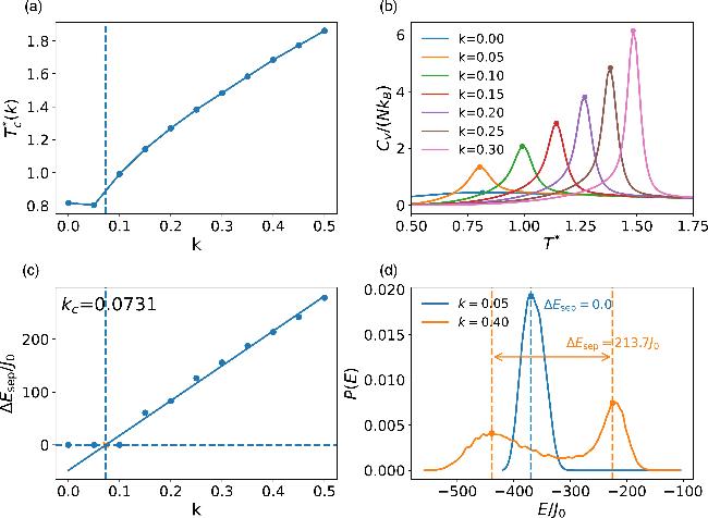
Figure 2. Validation of the MC simulations for the 1D intelligent Ising model. (a) Pseudo-critical temperature ${T}_{{\rm{c}}}^{* }(k)$ obtained from the peak position of the dimensionless specific heat ${C}_{V}/(N{k}_{{\rm{B}}})$ for a finite system. (b) Temperature dependence of the specific heat ${C}_{V}/(N{k}_{{\rm{B}}})$ for several representative values of k, where ${T}_{{\rm{c}}}^{* }(k)$ is identified as the temperature at which ${C}_{V}$ attains its maximum. The temperature is expressed in the reduced form ${T}^{* }$. (c) Energy separation ${\rm{\Delta }}{E}_{{\rm{sep}}}/{J}_{0}$ extracted from the energy probability distribution $P(E)$ along the pseudo-critical line ${T}^{* }={T}_{{\rm{c}}}^{* }(k)$. The solid line is a linear fit to the nonzero ${\rm{\Delta }}{E}_{{\rm{sep}}}/{J}_{0}$ data, and its intersection with ${\rm{\Delta }}{E}_{{\rm{sep}}}/{J}_{0}=0$ defines the tricritical coupling parameter ${k}_{{\rm{c}}}$. (d) Representative energy distributions $P(E)$ evaluated at $(k,{T}_{{\rm{c}}}^{* }(k))$ corresponding to the data points shown in (c). For $k\lt {k}_{{\rm{c}}}$, $P(E)$ exhibits a single-peak structure, whereas for $k\gt {k}_{{\rm{c}}}$ a clear double-peak structure is observed. The dashed vertical lines mark the peak positions used to define ${\rm{\Delta }}{E}_{{\rm{sep}}}$. |
As shown in figure 2(c), ${\rm{\Delta }}{E}_{{\rm{sep}}}$ increases approximately linearly with k in the first-order regime, and its extrapolation to zero provides an estimate of the critical coupling parameter ${k}_{{\rm{c}}}$ separating the two transition regimes. Note that both ${T}_{{\rm{c}}}(k)$ and ${k}_{{\rm{c}}}$ obtained here deviate from the values under thermodynamic limit due to the finite-size effect, but the consistent correspondence among the pseudo-critical line, the behavior of ${\rm{\Delta }}{E}_{{\rm{sep}}}$, and the structure of $P(E)$ demonstrate that the numerical simulations do capture the qualitative phase behavior described by the analytical solution in one dimension.
Simulation results for the 2D and 3D intelligent Ising models
Building on the 1D results, we next examine whether the tricritical scenario persists in higher dimensions and how the phase behavior depends on the coupling parameter k. The MC simulations are performed for both the 2D and 3D intelligent Ising models.
For the 2D system, the pseudo-critical temperature ${T}_{{\rm{c}}}^{* }(k)$, at which the specific heat reaches its maximal value, increases monotonically with k, as shown in figure 3(a). In the limit $k\to 0$, ${T}_{{\rm{c}}}^{* }$ approaches the critical temperature of the conventional 2D Ising model, while a larger value of k progressively shifts the phase transition to a higher temperature. Meanwhile, the specific-heat curves in figure 3(b) exhibit increasingly sharp peaks with increasing k, indicating enhanced energy fluctuations near the transition point. More importantly, the nature of the transition changes qualitatively as k increases. Along the pseudo-critical line ${T}^{* }={T}_{{\rm{c}}}^{* }(k)$, the energy probability distribution $P(E)$ evolves from a single-peak structure at a smaller k to a clear bimodal form at a larger k. This crossover is quantified by the energy separation ${\rm{\Delta }}{E}_{{\rm{sep}}}$ shown in figure 3(c). While ${\rm{\Delta }}{E}_{{\rm{sep}}}=0$ in the small k regime, a finite energy separation emerges beyond a threshold value of k and grows approximately linearly. Extrapolating the nonzero ${\rm{\Delta }}{E}_{{\rm{sep}}}$ to zero yields an estimate of the tricritical coupling parameter ${k}_{{\rm{c}}}$, which separates the continuous and discontinuous phase transition regimes.
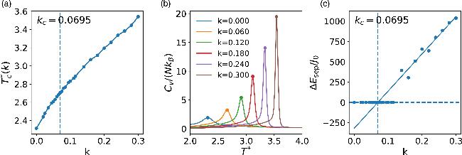
Figure 3. (a) Pseudo-critical temperature ${T}_{{\rm{c}}}^{* }(k)$ of the 2D intelligent Ising model as a function of the coupling parameter k obtained from the maximum of the specific heat. The vertical dashed line marks the tricritical coupling parameter ${k}_{{\rm{c}}}$ determined independently from the energy-separation analysis shown in panel (c). (b) Temperature dependence of the dimensionless specific heat ${C}_{V}/(N{k}_{{\rm{B}}})$ at some representative k values. For each curve, the peak position is indicated by a filled symbol. The temperature is expressed in the reduced form ${T}^{* }$. (c) Energy separation ${\rm{\Delta }}{E}_{{\rm{sep}}}/{J}_{0}$ extracted from the bimodal energy distribution as a function of k. The values below the threshold are set to zero, highlighting the emergence of a finite energy separation at large k values. The dashed horizontal line indicates ${\rm{\Delta }}{E}_{{\rm{sep}}}=0$ and the dashed vertical line denotes the tricritical coupling parameter ${k}_{{\rm{c}}}$ obtained by linear extrapolation of the nonzero data points. |
A similar phenomenology is observed in 3D. As shown in figure 4(a), the pseudo-critical temperature ${T}_{{\rm{c}}}^{* }(k)$ again increases with k and approaches the critical temperature of the conventional 3D Ising model in the limit $k\to 0$. The corresponding specific-heat curves in figure 4(b) display the same systematic sharpening with increasing k. Consistent with the two-dimensional case, the energy separation ${\rm{\Delta }}{E}_{{\rm{sep}}}$ extracted along the pseudo-critical line becomes finite above a threshold value of k and increases approximately linearly with k, as shown in figure 4(c). The resulting tricritical coupling parameter ${k}_{{\rm{c}}}$ marks the boundary between the continuous and discontinuous transitions.
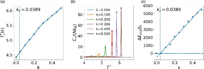
Figure 4. (a) Pseudo-critical temperature ${T}_{{\rm{c}}}^{* }(k)$ as a function of the coupling parameter k determined from the peak positions of the dimensionless specific heat ${C}_{V}/(N{k}_{{\rm{B}}})$. The vertical dashed line indicates the tricritical coupling parameter ${k}_{{\rm{c}}}$ obtained independently from the energy-separation analysis shown in (c). (b) Temperature dependence of the specific heat ${C}_{V}/(N{k}_{{\rm{B}}})$ at some representative k values, plotted as a function of the reduced temperature ${T}^{* }$. The peak position is marked by a filled symbol in each curve. (c) Energy separation ${\rm{\Delta }}{E}_{{\rm{sep}}}/{J}_{0}$ extracted from the energy probability distribution $P(E)$ along the pseudo-critical line ${T}^{* }={T}_{{\rm{c}}}^{* }(k)$. The values below the threshold are set to zero. The dashed horizontal line indicates ${\rm{\Delta }}{E}_{{\rm{sep}}}/{J}_{0}=0$, while the dashed vertical line marks the tricritical coupling parameter ${k}_{{\rm{c}}}$. The solid line represents a linear fit to the nonzero ${\rm{\Delta }}{E}_{{\rm{sep}}}/{J}_{0}$ data, whose extrapolated value at zero defines ${k}_{{\rm{c}}}$. |
Taking together, the results for both 2D and 3D closely parallel the analytical solution in 1D. The coupling parameter k not only shifts the transition temperature but also alters the order of the phase transition, giving rise to a tricritical point that connects the continuous and discontinuous phase transition regimes. These findings demonstrate that the tricritical behavior induced by the feedback-dependent coupling is robust across various spatial dimensions.
Mean-field solution
The mean-field theory provides further insight into the phase behavior of the intelligent Ising model across dimensions. Under the mean-field approximation, we substitute the mean-field decomposition ${s}_{i}=\phi +\delta {s}_{i}$ into the system's Hamiltonian, equation (2 ), where $\phi =\left\langle {s}_{i}\right\rangle $ is the average magnetization and $\delta {s}_{i}$ denotes the fluctuations. By assuming that the fluctuations are small, we can neglect the second-order and higher-order terms of $\delta {s}_{i}$. As detailed in the Methods section, the resulting free energy landscape can be written as
$\begin{eqnarray}\begin{array}{lll}f\left(\phi \right) & = & \displaystyle \frac{{z}^{2}{J}_{0}}{2}{\phi }^{2}\left(1+3k{\phi }^{2}\right)\\ & & -\,{k}_{{\rm{B}}}T\,{\mathrm{ln}}\left[2\,\cosh \left(\beta {J}_{0}z\left(\phi +2k{\phi }^{3}\right)\right)\right].\end{array}\end{eqnarray}$
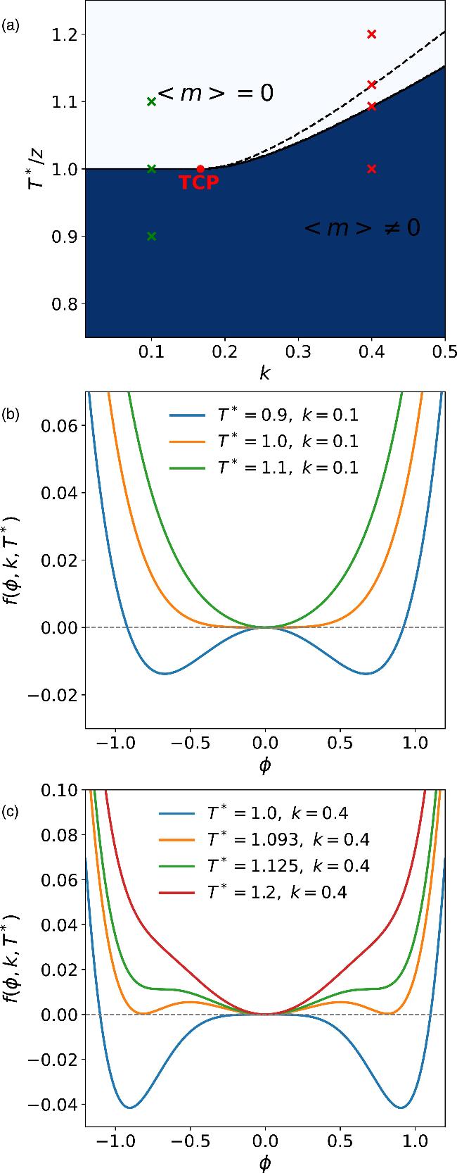
Figure 5(a) presents the phase diagram in the $\left(k,{T}^{* }/z\right)$ space derived from the mean-field theory. The reduced temperature ${T}^{* }/z$ is introduced to eliminate the coordination-number dependence inherent to the mean-field approximation. The white region indicates the paramagnetic phase ($\left\langle m\right\rangle =0$), the blue region represents the ferromagnetic phase ($\left\langle m\right\rangle \ne 0$), and the dashed line is the spinodal line. Expanding the free energy landscape near $\phi =0$, we obtain $\begin{eqnarray}\begin{array}{lll}f\left(\phi \right) & = & {f}_{0}+a\left(k,T\right){\phi }^{2}\\ & & \,+\,b\left(k,T\right){\phi }^{4}+c\left(k,T\right){\phi }^{6}+O\left({\phi }^{7}\right).\end{array}\end{eqnarray}$
The tricritical point can thus be determined by letting $a\left(k,T\right)=b\left(k,T\right)=0$, yielding ${k}_{{\rm{c}}}=\displaystyle \frac{1}{6},{T}_{{\rm{c}}}=z$. Figures 5(b) and (c) illustrate the free energy landscapes at different values of the coupling parameter $k$. At $k=0.1$, the system exhibits a continuous phase transition; while at $k=0.4$, the phase transition becomes discontinuous, clearly demonstrating the presence of a tricritical point.Although the phase diagram shows similar tricritical behavior for the mean-field model with the finite-dimensional models, there is a key difference that the continuous phase transition temperature ${T}_{{\rm{c}}}$ of the mean-field model does not depend on $k$, which might be attributed to the fact that the mean-field approximation greatly suppresses thermal fluctuations, especially around the critical points.
Figure 5. (a) Mean-field phase diagram in the $(k,{T}^{* }/z)$ space. The white and blue regions correspond to the paramagnetic ($\langle m\rangle =0$) and ferromagnetic ($\langle m\rangle \ne 0$) phases, respectively. The dashed line denotes the spinodal line, obtained from the mean-field free energy stability condition ${\partial }^{2}f/\partial {m}^{2}=0$. The red dot marks the tricritical point. (b) Mean-field free energy density $f(\phi ,k,T)$ for $k=0.1$ at some representative temperatures (green crosses in panel (a)), showing a continuous phase transition. (c) Mean-field free energy density $f(\phi ,k,T)$ for $k=0.4$ at some representative temperatures (red crosses in panel (a)), showing a discontinuous phase transition. |
Conclusions and discussion
Phase transitions in the intelligent Ising models
The study of the intelligent Ising model introduced in this work demonstrates how feedback mechanisms, realized through a magnetization-dependent coupling coefficient $J\left(m\right)$, can qualitatively change the phase behavior of the conventional Ising model. Both analytical derivation and MC simulation for the 1D system reveal the emergence of a tricritical point, where the nature of the phase transition changes from continuous (second-order) to discontinuous (first-order) as the nonlinear feedback parameter $k$ increases, in contrast to the phase behavior of the conventional 1D Ising model that no phase transitions appear at finite temperatures. In two and three dimensions, by MC simulation, we observe a similar phase transition behavior from continuous to discontinuous as $k$ increases. The mean-field theory confirms that the above phenomenon is dimension-independent, providing a generalized framework for understanding the tricriticality induced by the feedback mechanism in various dimensions.
In the conventional Ising model, the critical temperature increases with spatial dimension [23–26], and the critical behavior approaches the predictions of the mean-field theory as the dimension grows. We anticipate that the phase diagram in the $(k,T)$ space will similarly converge toward the mean-field result in higher dimensions. In our current simulations, important effects such as finite-size corrections, which are known to play a significant role in the Ising model, have not been systematically addressed. Future studies could employ algorithms more suited to exploring phase transitions, such as the Wang–Landau method [27], in combination with finite-size scaling analysis to determine the phase boundaries more precisely [28].
Sociophysical interpretation: opinion polarization induced by poll feedback
In our model, the nonlinear coupling $J={J}_{0}\left(1+k{m}^{2}\right)$ can be interpreted as a feedback mechanism induced by opinion polls during an election. As polling results become increasingly biased toward one side, the absolute magnetization $\left|m\right|$ increases, leading to a larger J, which enhances the tendency of individuals to align their opinions with their immediate social environment. Importantly, this does not imply a direct shift toward the poll-leading side, but rather a reinforcement of local consensus—a phenomenon similar to political homophily [29] or the echo chamber effect [30], where individuals become more influenced by surrounding opinions under perceived social pressure.
We consider a dynamic scenario where polling continues throughout the election period and individuals grow more responsive to these polls as the election day becomes closer [31, 32]. This temporal increase in poll sensitivity is modeled in the intelligent Ising model by a gradual increase in the feedback strength k. Initially, assuming a balanced race with $m=0$, the system remains disordered. As k increases, the system exhibits two qualitatively different behaviors depending on the temperature. At low temperatures, where fluctuations are relatively weak and individuals are more likely to retain being aligned with their local environment, the system undergoes a continuous phase transition: the order parameter m grows smoothly from zero, signaling a gradual polarization of public opinion. By contrast, at high temperatures, where individual opinions are more independent and fluctuations are strong, the system remains in a disordered state as k increases, until a critical threshold is reached. At this point, the system undergoes a discontinuous, first-order phase transition, and the magnetization m jumps abruptly away from zero, indicating a rapid, avalanche-like shift in collective opinion.
This behavior suggests a sociopolitical analogy: in more collectivistic societies (corresponding to low temperatures), collective opinion emerges progressively as individuals respond to local consensus under polling pressure. In more individualistic societies (high temperatures), opinions remain dispersed until polling influence becomes strong enough to trigger an opinion cascade [33]. Hence, our model captures two fundamentally different routes to consensus formation: smooth evolution and abrupt polarization, depending on the social temperature and feedback strength.
It is worth noting that the above interpretation is based on the analytical results of the 1D intelligent Ising model. In higher-dimensional systems, such as the 2D and 3D cases studied in our simulations, spontaneous symmetry breaking [34] occurs at low temperatures even without the feedback mechanism, leading to the emergence of collective opinion polarization. In these models, the system exhibits three qualitatively different regimes depending on temperature. At low temperatures, spontaneous ordering dominates; at intermediate and high temperatures, the behavior is similar to that observed in the 1D case, with the feedback strength $k$ controlling the onset and nature of polarization. This highlights the role of dimensionality in shaping the consensus formation process. In the Ising model, dimensionality reflects the extent of connectivity among individuals: higher dimensions correspond to individuals being influenced by a larger number of neighbors. This increased local interaction plays a significant role in facilitating the emergence of collective opinion, making dimensionality an important factor in the dynamics of consensus formation.
In summary, we incorporated feedback interactions into the conventional Ising model to build up an intelligent Ising model, leading to the emergence of complex phase behaviors. This model shows how adaptive interactions (a hallmark of intelligent matter) can qualitatively change phase transition behavior—enabling order to emerge where it otherwise would not, and tuning the nature of the transition between continuous and discontinuous. Our findings underscore that, in modern democratic processes, the way that information is disseminated can have subtle but profound effects on the aggregation of preferences. Understanding these effects is crucial for designing fair voting systems and for interpreting election results in an age of instant communication and social media influence.
Materials and methods
Exact solution of the 1D intelligent Ising model
To analyze the phase behavior of our model, we first introduce the free energy landscape as a function of magnetization $m$:
$\begin{eqnarray}F\left(m\right)=-{k}_{{\rm{B}}}T\,{\mathrm{ln}}\,{Z}_{N}\left(m\right),\end{eqnarray}$
where the partition function ${Z}_{N}\left(m\right)$ is defined as $\begin{eqnarray}{Z}_{N}\left(m\right)=\displaystyle \displaystyle \sum _{\left\{{s}_{i}\right\}}\delta \left(\displaystyle \frac{1}{N}\displaystyle \sum _{i=1}^{N}{s}_{i}-m\right)\exp \left[\beta J\left(m\right)\displaystyle \sum _{i=1}^{N}{s}_{i}{s}_{i+1}\right].\end{eqnarray}$
To evaluate ${Z}_{N}\left(m\right)$, we make use of the known solution for the conventional Ising model with an external magnetic field $h$ applied, whose Hamiltonian is13 ) can be alternatively written as
$\begin{eqnarray}H=-J\left(m\right)\displaystyle \displaystyle \sum _{\left\langle i,j\right\rangle }{s}_{i}{s}_{j}+h\displaystyle \displaystyle \sum _{i}{s}_{i}.\end{eqnarray}$
Its partition function is $\begin{eqnarray}\begin{array}{lll}{Z}_{{\rm{conv}}} & = & \exp \left(N\beta J\right)\left(\cosh \left(\beta h\right)\right.\\ & & {\left.+\,\sqrt{{\sinh }^{2}\left(\beta h\right)+\exp \left(-4\beta J\right)}\right)}^{N}.\end{array}\end{eqnarray}$
To relate it to ${Z}_{N}\left(m\right)$, we employ a mathematical transformation as described below. Equation ( $\begin{eqnarray}\begin{array}{lll}{Z}_{{\rm{conv}}}\left(\beta ,h\right) & = & \displaystyle {\int }_{-1}^{1}{\rm{d}}m\displaystyle \displaystyle \sum _{\left\{{s}_{i}\right\}}\delta \left(\displaystyle \frac{1}{N}\displaystyle \sum _{i=1}^{N}{s}_{i}-m\right)\\ & & \times \,\exp \left(\beta J\displaystyle \sum _{i=1}^{N}{s}_{i}{s}_{i+1}+\beta h\displaystyle \sum _{i=1}^{N}{s}_{i}\right)\\ & = & \displaystyle {\int }_{-1}^{1}{\rm{d}}m\exp \left[-\beta N{f}_{{\rm{conv}}}\left(\beta ,h,m\right)\right],\end{array}\end{eqnarray}$
which can be applied with the saddle point approximation in the thermodynamic limit to replace the integral by its value at the most probable magnetization ${m}^{\ast }$ to obtain $\begin{eqnarray}\begin{array}{lll}{Z}_{{\rm{conv}}}\left(\beta ,h\right) & \approx & \exp \left[-\beta N{f}_{{\rm{conv}}}\left(\beta ,h,{m}^{* }\right)\right]\\ & \approx & \displaystyle \displaystyle \sum _{\left\{{s}_{i}\right\}}\delta \left(\displaystyle \frac{1}{N}\displaystyle \displaystyle \sum _{i}{s}_{i}-{m}^{* }\right)\\ & & \times \,\exp \left(\beta J\displaystyle \sum _{i=1}^{N}{s}_{i}{s}_{i+1}\right)\exp \left(\beta hN{m}^{* }\right).\end{array}\end{eqnarray}$
Here, ${m}^{* }$ satisfies the equation of state for the conventional 1D Ising model under h: $\begin{eqnarray}\beta h\left(\beta ,{m}^{* }\right)=\,{\mathrm{ln}}\left(\sqrt{\displaystyle \frac{{m}^{* }}{1-{m}^{* }}}{{\rm{e}}}^{-2\beta J}+\sqrt{\displaystyle \frac{{m}^{* 2}}{1-{m}^{* 2}}{{\rm{e}}}^{-4\beta J}+1}\right).\end{eqnarray}$
Substituting the above expression for βh into equation (15 ), we eliminate the dependence on the external field h and obtain
$\begin{eqnarray}\begin{array}{c}\displaystyle \displaystyle \sum _{\left\{{s}_{i}\right\}}\delta \left(\displaystyle \frac{1}{N}\displaystyle \sum _{i=1}^{N}{s}_{i}-m\right)\exp \left(\beta J\displaystyle \sum _{i=1}^{N}{s}_{i}{s}_{i+1}\right)\\ \,={\left(\sqrt{{{\rm{e}}}^{2\beta J}{+{\rm{e}}}^{-2\beta J}\displaystyle \frac{{m}^{2}}{1-{m}^{2}}}+\displaystyle \frac{{{\rm{e}}}^{-\beta J}}{\sqrt{1-{m}^{2}}}\right)}^{N}\\ \,\times \,{\left({{\rm{e}}}^{-2\beta J}\displaystyle \frac{m}{\sqrt{1-{m}^{2}}}+\sqrt{1+{{\rm{e}}}^{-4\beta J}\displaystyle \frac{{m}^{2}}{1-{m}^{2}}}\right)}^{N}.\end{array}\end{eqnarray}$
Here we rewrite m* as m. This equation is purely mathematical, and remains valid when we generalize the coupling constant to be a function of magnetization, i.e. $J={J}_{0}\to J\left(m\right)={J}_{0}\left(1+k{m}^{2}\right)$. Therefore, the partition function of our feedback-regulated model becomes $\begin{eqnarray}\begin{array}{rcl}{{\rm{e}}}^{-\beta Nf\left(m\right)} & = & {Z}_{N}\left(m\right)\\ & = & {\left(\sqrt{{{\rm{e}}}^{2\beta J\left(m\right)}{+{\rm{e}}}^{-2\beta J\left(m\right)}\displaystyle \frac{{m}^{2}}{1-{m}^{2}}}+\displaystyle \frac{{{\rm{e}}}^{-\beta J\left(m\right)}}{\sqrt{1-{m}^{2}}}\right)}^{N}\\ & & \times \,{\left({{\rm{e}}}^{-2\beta J\left(m\right)}\displaystyle \frac{m}{\sqrt{1-{m}^{2}}}+\sqrt{1+{{\rm{e}}}^{-4\beta J\left(m\right)}\displaystyle \frac{{m}^{2}}{1-{m}^{2}}}\right)}^{N}.\end{array}\end{eqnarray}$
Taking the logarithm and being divided by $-\beta N$, we obtain the expression for the free energy landscape $\begin{eqnarray}\begin{array}{l}f\left(m\right)=-\frac{1}{\beta }\,{\mathrm{ln}}\left(\sqrt{{{\rm{e}}}^{2\beta J\left(m\right)}+{{\rm{e}}}^{-2\beta J\left(m\right)}\frac{{m}^{2}}{1-{m}^{2}}}+\frac{{{\rm{e}}}^{-\beta J\left(m\right)}}{\sqrt{1-{m}^{2}}}\right)\\ +\,\frac{m}{\beta }\,{\mathrm{ln}}\left({{\rm{e}}}^{-2\beta J\left(m\right)}\frac{m}{\sqrt{1-{m}^{2}}}+\sqrt{1+{{\rm{e}}}^{-4\beta J\left(m\right)}\frac{{m}^{2}}{1-{m}^{2}}}\right).\end{array}\end{eqnarray}$
This function forms the theoretical basis not only for this study, but also for future investigations of various intelligent matter models, including the identification of metastable states and the nature of phase transitions under different feedback mechanisms.MC simulation
To evolve the system toward thermal equilibrium, we adopted the conventional Metropolis algorithm with a key modification incorporating the feedback mechanism inherent to our intelligent Ising model in our MC simulations. In this model, the coupling coefficient is not a constant, but instead depends dynamically on the instantaneous magnetization $m$ by introducing a global feedback loop. Specifically, we define the coupling as $J\left(m\right)={J}_{0}\left(1+k{m}^{2}\right)$, where $k$ is the feedback strength.
At each MC step, a spin is randomly selected and proposed for flipping. To determine whether the flip should be accepted, we compute the corresponding energy change ΔE including both local and global contributions due to the feedback term. Let $m$ and $m^{\prime} $ be the system magnetizations before and after the flip, respectively, and ${\rm{\Delta }}J=k\left({m^{\prime} }^{2}-{m}^{2}\right){J}_{0}$ the resulting change in the coupling constant. The system energies before and after the flip can be respectively expressed as
$\begin{eqnarray}E=-J\displaystyle \displaystyle \sum _{\left\langle i,j\right\rangle }{s}_{i}{s}_{j},\end{eqnarray}$
and $\begin{eqnarray}E^{\prime} =-\left(J+{\rm{\Delta }}J\right)\displaystyle \displaystyle \sum _{\left\langle i,j\right\rangle }{s}_{i}{s}_{j}+2\left(J+{\rm{\Delta }}J\right){s}_{k}\displaystyle \displaystyle \sum _{j\in {\rm{nn}}\left(k\right)}{s}_{j},\end{eqnarray}$
where $\left\langle i,j\right\rangle $ denotes the summation over all nearest-neighbor spin pairs, and ${\rm{nn}}\left(k\right)$ represents the set of nearest neighbors of the flipping spin ${s}_{k}$. The second term in $E^{\prime} $ accounts for the change in interaction due to the flip of ${s}_{k}$, which only affects its local neighbors.The energy difference before and after the flip ${\rm{\Delta }}E=E^{\prime} -E$ is then
$\begin{eqnarray}{\rm{\Delta }}E=\displaystyle \frac{{\rm{\Delta }}J}{J}E+2\left(J+{\rm{\Delta }}J\right){s}_{k}\displaystyle \displaystyle \sum _{j\in {\rm{nn}}\left(k\right)}{s}_{j}.\end{eqnarray}$
This formulation avoids recomputing the full energy at every step and significantly improves computational efficiency, despite the involvement of a global coupling term through the feedback mechanism. The proposed flip is accepted with the probability $P=\,\min \left(1,{{\rm{e}}}^{-{\rm{\Delta }}E/{k}_{{\rm{B}}}T}\right)$, which ensures that the Markov chain satisfies the detailed balance and converges to the correct Boltzmann distribution.Numerical protocol
MC simulations were performed for the intelligent Ising model in one, two, and three spatial dimensions under periodic boundary conditions. All simulations employed the Metropolis single-spin–flip algorithm. One MC step corresponds to N attempted spin updates. To ensure ergodicity and facilitate transitions between symmetry-related magnetization states, a global spin–flip move was additionally attempted for every five sweeps. The simulated system sizes are: a chain of 400 spins for 1D, a square lattice of $30\times 30$ for 2D, and a cubic lattice of $12\times 12\times 12$ for 3D. The coupling parameter k is scanned in the range of $\left[0,0.05\right]$ with an increment of ${\rm{\Delta }}k=0.05$. The ranges of the temperature T are: $[0.2,2.2]$ in 1D, $[2.0,4.5]$ in 2D, and $[4.0,6.7]$ in 3D, and the temperature interval is smaller when T is closer to the transition temperature ${T}_{{\rm{c}}}$. For each state point $(k,{T}^{* })$, simulations were run for 108 MC steps. All systems started from random configurations corresponding to a near-zero initial magnetization. The first 30% of the trajectory was discarded for equilibration and thermodynamic observables were measured from the remaining equilibrated configurations.
Data analysis
All data analysis was carried out in dimensionless units by measuring energies in the unit of the baseline coupling ${J}_{0}$ and temperatures in the unit of ${J}_{0}/{k}_{{\rm{B}}}$. In this section, E and T denote the dimensionless total energy and temperature, respectively. The raw simulation outputs were first organized by a pair of parameters $\left(k,{T}_{i}\right)$ and then grouped according to the coupling parameter k. The sampled energy values at every ${T}_{i}$ were pooled for subsequent analysis after discarding the equilibration steps. The multistate Bennett acceptance ratio (MBAR) method [35] was employed to obtain thermodynamic quantities at a continuous temperature T for a fixed k. The MBAR combines all energy samples collected at multiple temperatures $\{{T}_{i}\}$ into a statistically consistent estimator and enables the evaluation of the ensemble averages at an arbitrary target temperature T within the temperature range covered by the simulated states. The energy probability distribution at a fixed k, denoted as ${P}_{k}(E;T)$, was reconstructed by forming a normalized weighted histogram of the pooled energy samples. The same reweighted distribution was used to compute the first moment ${\langle E\rangle }_{T}$ and the second moment ${\langle {E}^{2}\rangle }_{T}$ of the total energy.
The heat capacity per spin was then evaluated from the standard fluctuation formula
$\begin{eqnarray}{C}_{V}(T)=\displaystyle \frac{1}{N{T}^{2}}\left({\langle {E}^{2}\rangle }_{T}-{\langle E\rangle }_{T}^{2}\right),\end{eqnarray}$
where N is the total number of spins. For each fixed k and system size L, the pseudo-critical temperature ${T}_{{\rm{c}}}(k;L)$ was defined as the temperature at which ${C}_{V}(T)$ reaches its maximum.The energy separation ${\rm{\Delta }}{E}_{{\rm{sep}}}$ was used as a quantitative indicator of phase coexistence. For each fixed coupling parameter k, ${\rm{\Delta }}{E}_{{\rm{sep}}}$ was evaluated at ${T}_{{\rm{c}}}(k)$, at which the energy probability distribution ${P}_{k}(E;{T}_{{\rm{c}}})$ was reconstructed using the MBAR and represented as a weighted energy histogram. The histogram was smoothed using a Gaussian kernel with a finite width before peak analysis to suppress the noise. If the resulting ${P}_{k}(E;{T}_{{\rm{c}}})$ exhibits a bimodal structure, ${\rm{\Delta }}{E}_{{\rm{sep}}}$ is defined as the energy difference between the positions of the two dominant peaks. A bimodal classification was accepted only when additional quantitative criteria on the minimum peak separation, the relative heights of the two peaks, and the suppression of the probability at the valley between the peaks were simultaneously satisfied. If these criteria were not met, or if ${P}_{k}(E;{T}_{{\rm{c}}})$ shows only a single peak, ${\rm{\Delta }}{E}_{{\rm{sep}}}$ was set to zero.
Mean-field solution
In our model, the coupling coefficient J depends on the average magnetization of the system, and the Hamiltonian is written as
$\begin{eqnarray}\begin{array}{lll}H\left(\left\{{s}_{i}\right\}\right) & = & -{J}_{0}\left(1+k{m}^{2}\right)\displaystyle \displaystyle \sum _{\left\langle i,j\right\rangle }{s}_{i}{s}_{j}\\ & = & -{J}_{0}\left[1+\displaystyle \frac{k}{{N}^{2}}{\left(\displaystyle \sum _{i=1}^{N}{s}_{i}\right)}^{2}\right]\displaystyle \displaystyle \sum _{\left\langle i,j\right\rangle }{s}_{i}{s}_{j},\end{array}\end{eqnarray}$
where $m=\displaystyle \frac{1}{N}\displaystyle {\sum }_{i=1}^{N}{s}_{i}$ is the average spin of the system. In the mean-field approximation, each spin ${s}_{i}$ is decomposed into its average value $\phi =\left\langle {s}_{i}\right\rangle $ and a fluctuation term $\delta {s}_{i}$: $\begin{eqnarray}{s}_{i}=\phi +\delta {s}_{i}.\end{eqnarray}$
Assuming the fluctuation is small, we retain only the first-order terms in $\delta {s}_{i}$ and neglect higher-order contributions.Expanding the term ${\left(\displaystyle {\sum }_{i=1}^{N}{s}_{i}\right)}^{2}$, we obtain
$\begin{eqnarray}{\left(\displaystyle \sum _{i=1}^{N}{s}_{i}\right)}^{2}=-N\left(N-1\right){\phi }^{2}+2\left(N-1\right)\phi \displaystyle \sum _{i=1}^{N}{s}_{i}.\end{eqnarray}$
Substituting this into the expression for J, we get $\begin{eqnarray}J\approx {J}_{0}\left(1-k{\phi }^{2}+2k\phi m\right).\end{eqnarray}$
Considering that the total number of nearest-neighbor spin pairs is $\displaystyle \frac{zN}{2}$, the two-spin interaction term under the mean-field approximation becomes $\begin{eqnarray}\displaystyle \displaystyle \sum _{\left\langle i,j\right\rangle }{s}_{i}{s}_{j}\approx \displaystyle \frac{zN}{2}{\phi }^{2}+z\phi \displaystyle \sum _{i=1}^{N}\delta {s}_{i}.\end{eqnarray}$
By combining the above expansions together, the Hamiltonian is reduced to a form containing only single-spin terms as $\begin{eqnarray}H\approx \displaystyle \frac{z{J}_{0}N}{2}\left({\phi }^{2}+3k{\phi }^{4}\right)-z{J}_{0}\left(\phi +2k{\phi }^{3}\right)\displaystyle \sum _{i=1}^{N}{s}_{i}.\end{eqnarray}$
As the Hamiltonian now only contains independent single-spin terms, the partition function becomes $\begin{eqnarray}\begin{array}{lll}{Z}_{N} & = & \displaystyle \displaystyle \sum _{\left\{{s}_{i}\right\}}\exp \left(-\beta H\right)\\ & = & \exp \left[-\beta \displaystyle \frac{z{J}_{0}N}{2}\left({\phi }^{2}+3k{\phi }^{4}\right)\right]\\ & & \times \,\displaystyle \prod _{i=1}^{N}\displaystyle \displaystyle \sum _{{s}_{i}=\pm 1}\exp \left[\beta z{J}_{0}\left(\phi +2k{\phi }^{3}\right){s}_{i}\right]\\ & = & \exp \left[-\beta {J}_{0}\displaystyle \frac{zN}{2}\left({\phi }^{2}+3k{\phi }^{4}\right)\right]\\ & & {\left[\times \,[2\,\cosh \left(\beta z{J}_{0}\left(\phi +2k{\phi }^{3}\right)\right)\right]}^{N}.\end{array}\end{eqnarray}$
The mean-field free energy density is thus given by $\begin{eqnarray}\begin{array}{lll}f\left(\phi \right) & = & -\displaystyle \frac{1}{\beta N}\,{\mathrm{ln}}\,{Z}_{N}\\ & = & \displaystyle \frac{z{J}_{0}}{2}{\phi }^{2}\left(1+3k{\phi }^{2}\right)\\ & & -\,{k}_{{\rm{B}}}T\,{\mathrm{ln}}\left[2\,\cosh \left(\beta {J}_{0}z\left(\phi +2k{\phi }^{3}\right)\right)\right].\end{array}\end{eqnarray}$
Expanding the free energy near φ = 0 as a Taylor series yields $\begin{eqnarray}f\left(\phi \right)={f}_{0}+a\left(k,T\right){\phi }^{2}+b\left(k,T\right){\phi }^{4}+c\left(k,T\right){\phi }^{6}+O\left({\phi }^{7}\right).\end{eqnarray}$
By analyzing the behavior of these coefficients, we obtain the phase diagram of the system. In particular, the change of the sign in the coefficient of the quartic term $b(k,T)$ indicates the presence of a tricritical point, where the nature of the phase transition changes from second-order to first-order as k increases.