


1. Introduction
The intricate and often unpredictable nature of chaotic systems, coupled with their prevalence across a wide array of real-world phenomena, has long captivated the attention of researchers, driving extensive and in-depth investigations into their underlying dynamics [1–5]. Recent advancements in the study of chaotic systems have led to the development of increasingly sophisticated analysis techniques, grounded in a robust statistical description framework of the natural measure [6], which weighs the long-term asymptotic behavior on chaotic attractors [7]. The evaluation of averages of various variables, which elucidates macroscopic properties of the system, demands an accurate characterization of the natural measure.
The natural measure is supported on the possibly fractal structure of an attractor, and hence the explicit analytical expression is generally elusive. Unstable periodic orbits (UPOs, also called cycles), instead, may serve as a ‘skeleton' of chaotic dynamics, encapsulating a wealth of dynamical information [8–10]. Cycle expansions, by systematically organizing the set of UPOs in a hierarchical manner, bridge the gap between the global natural measure and local dynamical properties. This technique enables a layered approximation of the natural measure and emerges as a powerful theoretical framework for a quantitative analysis of chaotic systems, when combined with symbolic dynamics [11] and cycle search algorithms [12–17]. Importantly, observable averages can be accurately calculated using only a small number of cycles [18].
In strongly hyperbolic chaotic systems, averages of observables converge exponentially with increasing cycle length due to the shadowing property [7, 19]. However, ubiquitous non-hyperbolicity in physical systems often leads to slow convergence in cycle expansions, limiting their applicability [20]. This usually induces singularities in the natural measure, where the stability eigenvalues of UPOs scale algebraically with topological length (in case of intermittency) near the folding points or their images. Such singularities may not be well captured by a small number of cycles and thus severely degrade the convergence of cycle expansions.
To address this trouble, various techniques have been designed but only make limited improvements, since the singularities are still not accurately quantified. For example, one may [21, 22] derive certain spectral determinant from the distribution of evolution time in hyperbolic regions of intermittent systems, but the accuracy of this approach is poor. Stability ordering scheme [23] may serve as an alternative, converging faster than traditional topological length truncation in non-hyperbolic systems. However, this method requires the stabilities of a large number of long UPOs, and improper stability truncation could lead to huge errors. Infinite symbolic alphabets [24] could be established and used to estimate the fundamental terms of cycle expansion through tail resummation, analytic continuation, or integral transformation. However, this method fails to yield an analytical asymptotic estimate for curvature corrections, leading to substantial numerical errors and limiting its value to purely theoretical interest. The conjugate scheme [25] accelerates the convergence by performing cycle expansion in the conjugate hyperbolic system, while only a very small number of systems have suitable conjugate systems. The induced map [26] reconstructs the natural measures for the singular and non-singular parts using analytic approximation and cycle expansion, respectively, thereby improving computational accuracy and convergence. However, the scheme is relatively computationally intensive and applicable only to one-dimensional intermittent maps. Consequently, based on cycle expansions, it is of paramount importance to develop a program that can be more extensively applied to dynamical systems with a singular natural measure.
The critical issue here is: how to maintain the rapid convergence of the cycle expansion while constructing a computational framework applicable to systems with singular natural measure caused by non-uniform hyperbolicity? In this paper, a novel layered approximation algorithm is proposed to account for the above considerations. It not only addresses the slow convergence of cycle expansions in singular systems but also provides a new perspective for understanding how singularities affect the overall statistical properties, which is of great significance for studying complex non-equilibrium systems.
This paper is organized as follows. Section 2 explores the physical picture, theoretical foundations, and detailed algorithmic aspects of the layered approximation scheme. To verify its effectiveness and generality, section 3 applies it to several typical chaotic systems featuring singular natural measures: those with intermittency, with multiple singularities, or with infinitely many singularities. Finally, section 4 discusses possible improvements and potential applications of the algorithm.
2. A layered scheme
Cycle expansions with finite truncations constitute a hierarchical linear approximation of the dynamics [27]. Local information from densely distributed UPOs approximates the natural measure—a process possibly compromised in non-hyperbolic systems. Slow convergence arises from the failure of the approximation with finite number of cycles to capture singularities in the measure. To address this, we propose a layered decomposition of the natural measure into: (i) singular layers: governed by the distribution of singular points, directly responsible for slow convergence. (ii) Hyperbolic layers: the residual smooth component, being approximated by the natural measure $\tilde{\rho }(x)$ of selected hyperbolic system $\tilde{f}(x)$. $\tilde{f}(x)$ should be topologically conjugated, not necessarily smoothly. The conjugacy is constructed to preserve the symbolic dynamics and the phase-space structure (e.g. the ordering of critical points and their images). Any hyperbolic system whose symbolic dynamics and kneading sequence [7] match those of the original system is acceptable. This decomposition enables rapid convergence in cycle expansions by isolating singularities from hyperbolic dynamics. However, poorly chosen conjugates that alter the kneading sequence may lead to convergence failure.
To validate the hierarchical algorithm and showcase its core principles with maximal clarity and minimal computational cost, we examine a set of prototypical unimodal maps whose natural measures carry distinct singularities. Although one-dimensional, these maps capture concrete physical and biological processes: the logistic-like map governs population dynamics in ecology [28], whereas the intermittent map reproduces the alternation of long laminar intervals and sparse turbulent bursts observed in fluid flows [29]. The Feray-like map has a singularity at x = 0 [as shown in figures 1(a) and (b)]2 ). The map ${f}_{3s}(x)=\,\rm{sin}\,(\frac{\pi }{a}-\frac{\pi }{a}x),a=1.315644...$ extremely compresses the phase space in the neighborhood of the critical point $x=1-\frac{a}{2}$, making a singularity at x = 1, while $\tilde{\rho }(x)$ may be derived from a linear map:
$\begin{eqnarray}{f}_{1s}(x)=\left\{\begin{array}{ll}\frac{x}{(1-\sqrt{x/2})}, & \,x\in [0,\frac{1}{2})\\ 2-2x, & \,x\in [\frac{1}{2},1]\end{array}\right.,\end{eqnarray}$
which presents the intermittency as f1s(x) → x + cx1+s, x → 0+, s ∈ (0, 1). The choice of hyperbolic system is non-unique and a practical criterion is to select the simplest piecewise-linear map that (i) preserves the topological entropy and kneading invariants of the original system and (ii) produces a hyperbolic natural measure whose overall shape resembles the singular natural measure with its singular spike removed. The $\tilde{\rho }(x)$ may be derived from the tent map: $\begin{eqnarray}\tilde{f}(x)=\left\{\begin{array}{ll}2x,\quad & \,x\in [0,\frac{1}{2}]\\ 2-2x,\quad & \,x\in (\frac{1}{2},1]\end{array}\right.,\end{eqnarray}$
which has a uniform measure. The logistic map f2s(x) = 4x(1 − x) has two singularities at x = 0 and x = 1 [as shown in figures 1(c) and (d)], while $\tilde{\rho }(x)$ can also be derived from the tent map ( $\begin{eqnarray}{\tilde{f}}_{3s}(x)=\left\{\begin{array}{ll}{x}_{a}+\frac{1-{x}_{a}}{{x}_{b}}x,\quad & \quad x\in [0,{x}_{b})\\ \frac{1}{{x}_{b}-1}(x-1),\quad & \quad x\in [{x}_{b},1]\end{array}\right.,\end{eqnarray}$
where ${x}_{a}=\,\rm{sin}\,\frac{\pi }{a}=0.684355...$ and xb = 0.538 770… The image of x = 0 is a fixed point xa for both maps f3s(x) and ${\tilde{f}}_{3s}(x)$, which induces three singularities x = 1, 0, xa in the natural measure, as shown in figures 1(e) and (f). The map ${f}_{4s}(x)=\,\rm{sin}\,(\frac{\pi }{a}-\frac{\pi }{a}x),\,a=1.102634...$ extremely compresses the phase space at $x=1-\frac{a}{2}$ and induces four singularities in the natural measure at x = 1, 0, xa, xb, with ${f}_{4s}(1-\frac{a}{2})=1$, f4s(1) = 0, f4s(0) = xa = f4s(xb) and f4s(xa) = xb. Clearly, x = xa and x = xb constitutes a period-2 cycle $\overline{{x}_{a}{x}_{b}}$. The $\tilde{\rho }(x)$ may be derived from a linear map: $\begin{eqnarray}{\tilde{f}}_{4s}(x)=\left\{\begin{array}{ll}{x}_{a}+\frac{1-{x}_{a}}{{x}_{d}}x,\quad & x\in [0,{x}_{d})\\ \frac{({x}_{b}-1-{x}_{a}{x}_{b}-{x}_{a})\cdot (x-{x}_{d})}{({x}_{b}-1)({x}_{d}-{x}_{b})}+1,\quad & x\in [{x}_{d},{x}_{b})\\ \frac{{x}_{a}}{{x}_{b}+1}(x-1),\quad & x\in [{x}_{b},1]\\ \quad \end{array}\right.,\end{eqnarray}$
where xa = 0.288 273… , xb = 0.897 365… , xd = 0.336 848… , as shown in figures 1(g) and (h).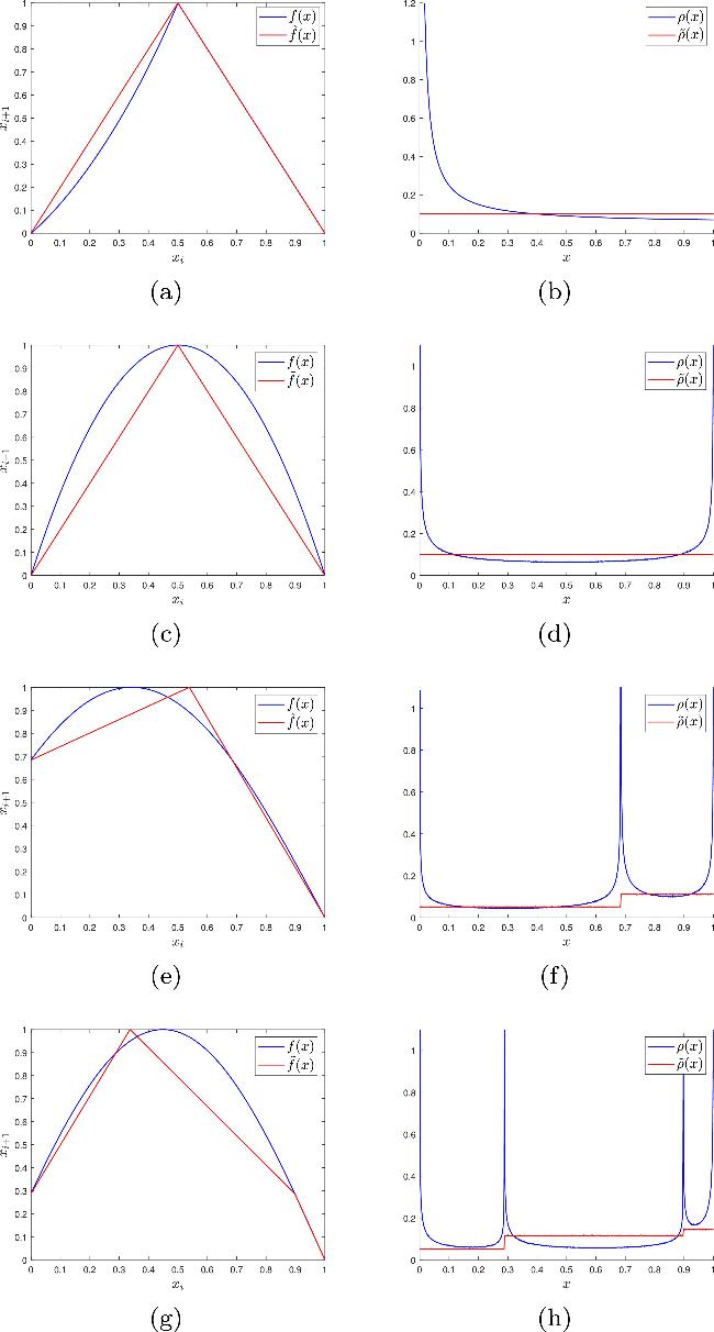
Figure 1. Systems with singular natural measure and their hyperbolic analogues. (a), (c), (e), (g) The non-hyperbolic dynamics f(x) (blue solid line) with different numbers of singularities and the corresponding hyperbolic system $\tilde{f}(x)$ (red solid line). (b), (d), (f), (h) The hyperbolic layer of non-hyperbolic systems can be well approximated by the conjugate natural measure $\tilde{\rho }(x)$ (red solid line, which are typically rather flat) with the correction function C(x). The four pairs of subfigures correspond to the systems of one, two, three, and four singularities, respectively. The smooth natural measure curves were likewise produced by long-time Monte-Carlo simulation: the one-dimensional phase space was partitioned into small intervals and the visitation frequency of the trajectory within each bin was recorded to yield the histogram shown. |
For any one-dimensional system with a singular natural measure, we may select a hyperbolic map preserving the phase space structure. Singularities arise from the extreme compression of phase space or intermittency, their locations can therefore be inferred directly from the dynamics f(x). The asymptotic form of singularities is analytically derivable from the evolution equation of the natural measure:
$\begin{eqnarray}\rho (x)=\displaystyle \sum _{i}\frac{\rho ({x}_{i})}{| {f}^{{\prime} }({x}_{i})| },\end{eqnarray}$
where xi = f−1(x) is the ith preimage of x and ${f}^{{\prime} }({x}_{i})$ is the stability factor at xi. The associated singularity exponent is obtained by matching the orders of x on both sides of the equation. By combining the singular layers with a hyperbolic layer—expanded as a correction function C(x) that acts on the measure $\tilde{\rho }(x)$ of a chosen hyperbolic system whose cycle expansion converges exponentially—we obtain a high-fidelity approximation of the original measure. This enables efficient computation of observable averages well beyond the reach of conventional cycle expansion.We demonstrate our framework using a prototype system with a singular natural measure (see figure 2), featuring two singularities at xa and xb. We can decompose the measure into four singular layers ${\{{\rho }_{i}(x)\}}_{i=1}^{4}$ and one hyperbolic layer ρ0(x). The asymptotic behavior of each singular layer admits explicit analytical approximation:
$\begin{eqnarray}{\rho }_{i}(x)=\left\{\begin{array}{l}{c}_{{s}_{i}}| x-{x}_{a,b}{| }^{-{s}_{i}},x\in [0,{x}_{a,b}){\rm{or}}({x}_{a,b},1]\quad \\ \quad \quad \quad 0,\quad \qquad x\in [{x}_{a,b},1]{\rm{or}}[0,{x}_{a,b}]\end{array}\right.,\end{eqnarray}$
where the position and the singularity exponent si for each singular layer are analytically determined from f(x). For the hyperbolic layer, we write ${\rho }_{0}(x)=C(x)\tilde{\rho }(x)$, where $\tilde{\rho }(x)$ is the natural measure of a conjugate hyperbolic system. Although C(x) is initially unknown, it admits a spectral expansion in terms of orthogonal polynomials. The full natural measure then decomposes as: $\begin{eqnarray}\rho (x)=\left\{\begin{array}{l}{c}_{{s}_{1}}{({x}_{a}-x)}^{-{s}_{1}}+{c}_{{s}_{3}}{({x}_{b}-x)}^{-{s}_{3}}\quad \\ +\displaystyle \sum _{l=0}^{n}{c}_{l}{P}_{l}(\varphi (x))\tilde{\rho }(x),\quad x\in [0,{x}_{a})\quad \\ {c}_{{s}_{2}}{(x-{x}_{a})}^{-{s}_{2}}+{c}_{{s}_{3}}{({x}_{b}-x)}^{-{s}_{3}}\quad \\ +\displaystyle \sum _{l=0}^{n}{c}_{l}{P}_{l}(\varphi (x))\tilde{\rho }(x),\quad x\in [{x}_{a},{x}_{b}),\quad \\ {c}_{{s}_{2}}{(x-{x}_{a})}^{-{s}_{2}}+{c}_{{s}_{4}}{(x-{x}_{b})}^{-{s}_{4}}\quad \\ +\displaystyle \sum _{l=0}^{n}{c}_{l}{P}_{l}(\varphi (x))\tilde{\rho }(x),\quad x\in [{x}_{b},1]\quad \end{array}\right.\end{eqnarray}$
where the correction function is expanded as $C(x)\,={\sum }_{l}^{n}{c}_{l}{P}_{l}(\varphi (x))$. Away from the corresponding singularity, the singular layer ρi(x) is negligibly small and readily cancelled by C(x). {Pl(x)} are the lth order Legendre orthogonal polynomials [30] and ${\{{c}_{l}\}}_{l=0}^{n}$ are the Legendre coefficients. φ(x) = 2x − 1 is a shift-and-scale function and maps phase space interval [0, 1] onto the canonical orthogonal interval [−1, 1] required by Legendre polynomials. The singularity exponents ${\{{s}_{i}\}}_{i=1}^{4}$ can be analytically approximated from the measures in the neighborhoods of the pre-images. The coefficients ${\{{c}_{{s}_{i}}\}}_{i=1}^{4}$ (singular layers) and {cl} (hyperbolic layer) may be computed numerically. Leveraging the exponential convergence in hyperbolic systems, this transforms the natural measure determination to the evaluation of these coefficients with several exact constraints imposed by: (i) the measure normalization: ${\int }_{{ \mathcal M }}\rho (x){\rm{d}}x=1$. (ii) The dynamical invariance of the natural measure: ⟨a⟩ = ⟨a∘f⟩ for any observable a(x) and the natural measure ρ(x) of the dynamics xn+1 = f(xn). This is derived from the conjugacy of the Koopman operator ${ \mathcal K }$ [31] and the Perron–Fröbenius operator ${{ \mathcal L }}_{{\rm{P}}{\rm{F}}}$ [7] under ergodic evolution: $\begin{eqnarray}\begin{array}{rcl}{\displaystyle \int }_{{ \mathcal M }}\rho (x)a(f(x)){\rm{d}}x & = & {\displaystyle \int }_{{ \mathcal M }}\rho (x)[{ \mathcal K }\circ a](x){\rm{d}}x\\ & = & {\displaystyle \int }_{{ \mathcal M }}[{{ \mathcal L }}_{{\rm{P}}{\rm{F}}}\circ \rho ](x)a(x){\rm{d}}x\\ & = & {\displaystyle \int }_{{ \mathcal M }}\rho (x)a(x){\rm{d}}x.\end{array}\end{eqnarray}$
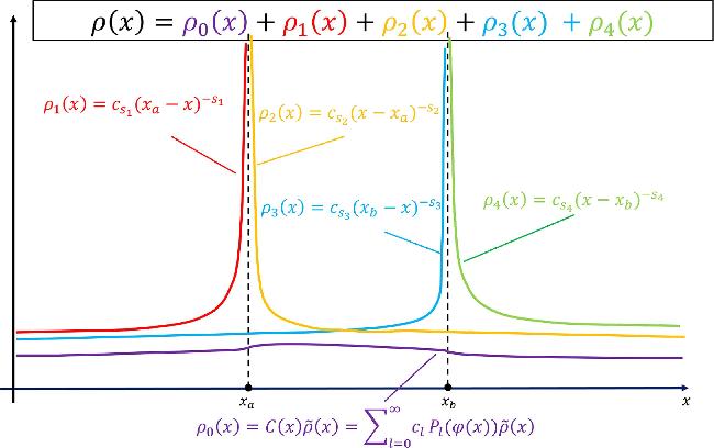
Figure 2. The natural measure ρ(x) of a system with two singular points is decomposed into a hyperbolic layer ρ0(x) and four singular layers ${\{{\rho }_{i}(x)\}}_{i=1}^{4}$. Each layer and its analytic expression are color-coded: the singular layers contain the coefficient ${c}_{{s}_{i}}$ and the singularity exponent si, whereas the hyperbolic layer is accurately approximated by the conjugate natural measure $\tilde{\rho }(x)$ and a correction function C(x). |
This time-invariance principle, which is intuitive from ergodicity and rigorously established via operator conjugacy, provides critical cues for high-precision measure approximation. Crucially, each observable ak(x) generates an independent equation:
$\begin{eqnarray}\langle {a}_{k}\rangle =\langle {a}_{k}\circ f\rangle ,\end{eqnarray}$
sufficiently many of which is able to determine all $\{{c}_{{s}_{i}}\}$ and {cl}. The convergence rate of our scheme depends on the smoothness of the chosen observables {ak(x)}. Smooth observables (e.g. orthogonal polynomials) typically yield faster convergence, while observables with singularities may require more expansion terms The target observable average is then: $\begin{eqnarray}\begin{array}{rcl}\langle a(x)\rangle & = & \displaystyle \sum _{i}{c}_{{s}_{i}}{\langle a(x)\rangle }_{{\rho }_{i}}+\displaystyle \sum _{l=0}^{n}{c}_{l}{\langle {\tilde{a}}_{l}(x)\rangle }_{\tilde{\rho }}\\ & = & \displaystyle \sum _{i}{c}_{{s}_{i}}{\displaystyle \int }_{{ \mathcal M }}a(x){\rho }_{i}(x){\rm{d}}x+\displaystyle \sum _{l=0}^{n}{c}_{l}\frac{{\sum }_{\tilde{p}}{A}_{\tilde{p},l}{z}^{{T}_{\tilde{p}}}| {{\rm{\Lambda }}}_{\tilde{p}}| }{{\sum }_{\tilde{p}}{T}_{\tilde{p}}{z}^{{T}_{\tilde{p}}}| {{\rm{\Lambda }}}_{\tilde{p}}| },\end{array}\end{eqnarray}$
where the modified observable ${\tilde{a}}_{l}(x)={P}_{l}(\varphi (x))a(x)$ admits efficient computation of $\langle {\tilde{a}}_{l}\rangle $ via rapidly converging cycle expansions [7, 18] (the second term) in the selected hyperbolic system $\tilde{f}(x)$. The second term sums over the combination of all prime cycles and all pseudo-cycles [7]) $\tilde{p}$ of $\tilde{f}(x)$ up to the truncation length ${t}_{{\rm{\max }}}$. Correspondingly, ${A}_{\tilde{p},l}={\sum }_{{x}_{i}\in \tilde{p}}{\tilde{a}}_{l}({x}_{i})$ and ${T}_{\tilde{p}}$, respectively, denote the cumulant observable and the period associated with $\tilde{p}$. The truncation length tmax denotes the maximum topological length of prime cycles or pseudo-cycles retained in the cycle expansion; equivalently, all orbits whose period ${T}_{p}\leqslant {t}_{{\rm{\max }}}$ are included. This cut-off is independent of the expansion order n used for the correction function C(x).3. Numerical results
We test the effectiveness of the layered scheme in several example systems and compare it with existing methods. In the numerical experiments, the convergence rates are assessed through a dual-validation mechanism. The averages obtained with the expansion order n + 1 are used as the benchmark values when estimating the logarithmic errors with the expansion order not greater than n. Any observable a(x) can be substituted into our framework and we focused on ⟨x⟩ for clarity and consistency across examples. Moreover, the averages were also computed independently via long-time Monte-Carlo integration [32] to ensure convergence to the correct value. The Monte Carlo validation employs a single trajectory of 109 steps, after discarding 107 transient steps, starting from a randomly chosen typical point x0 in phase space for each system. Expectation values are computed as
$\begin{eqnarray}{\langle x\rangle }_{{\rm{M}}{\rm{C}}}=\frac{1}{1{0}^{9}}\displaystyle \sum _{i=1{0}^{7}+1}^{1{0}^{9}+1{0}^{7}}{x}_{i},\quad {x}_{i}={f}^{i}({x}_{0}).\end{eqnarray}$
Figures 3(a) and (b) demonstrate accelerated convergence via our layered scheme for the Feray-like map (1 ). The natural measure at x = 0 (ρ(x) ∼ csx−s as x → 0+, $s=\frac{1}{2}$) decomposes into a singular layer and a hyperbolic layer where the tent map (2 ) is selected as the hyperbolic replacement. Equation (10 ) can thus be rewritten as: 9 ) with n + 2 independent observables, e.g. {1, x, x2, …, xn+1}. Observable averages converge rapidly with the expansion order n until a critical threshold $\hat{n}$. Beyond $\hat{n}$, the errors increase rather than decrease with the increase of n. Crucially, $\hat{n}$ increases with the truncation length tmax, enabling precision control through parameter selection. Here, it is easy to check from figure 3 that the threshold $\hat{n}$ corresponding to each tmax, is $\hat{n}\approx {t}_{\,\rm{max}\,}-3$. In fact, we may provide a reliable heuristic for parameter selection that $\hat{n}\propto \frac{{t}_{\,\rm{max}\,}}{1.5}$ for the Feray-like map. The relationship is not universal but follows a predictable pattern based on the nonlinearity of f(x). The scaling law $\hat{n}\propto \frac{{t}_{\,\rm{max}\,}}{m}$ depends on the map's local degree m near critical points: m = 1.5 for Feray-like maps, m = 2 for quadratic maps, m = 3 for cubic maps, etc. This exponent m reflects how rapidly the map stretches phase space near singularities. For observables, smoother polynomial bases yield better convergence than non-analytic functions. The relationship is therefore map-dependent but observable-class universal within the same smoothness category. The theoretical explanation for the existence of the threshold $\hat{n}$ is rooted in the term ⟨a∘f⟩ in equation (9 ), which is employed to determine the expansion coefficients ${\{{c}_{l}\}}_{l=0}^{n}$. The cycle expansion of ⟨a∘f⟩ can only resolve polynomial observables up to a certain order for the dynamics f(x). Given a specific truncation length ${\hat{t}}_{\,\rm{max}\,}$, the most wavy cycle of this length contains $[\frac{{t}_{\,\rm{max}\,}}{1.5}]$ peaks ([… ] denotes the floor function.), which may capture all the wavy profiles of polynomials of order tmax. For this reason, the cycle expansion of ⟨a∘f⟩ can only be effective for a polynomial observable a(x) of order $[\frac{{\hat{t}}_{\,\rm{max}\,}}{1.5}]$ if f(x) is the Feray-like map (order $[\frac{{\hat{t}}_{\,\rm{max}\,}}{2}]$ for quadratic maps, order $[\frac{{\hat{t}}_{\,\rm{max}\,}}{3}]$ for cubic maps and so on). We observed a larger $\hat{n}$ probably because of the existence of pseudo cycles [7, 9, 18], which shadow long cycles with shorter ones.
$\begin{eqnarray}\langle a(x)\rangle ={c}_{{s}_{1}}{\langle a(x)\rangle }_{{\rho }_{1}}+\displaystyle \sum _{l=0}^{n}{c}_{l}{\langle {\tilde{a}}_{l}(x)\rangle }_{\tilde{\rho }},\end{eqnarray}$
where $\tilde{\rho }(x)$ is the natural measure of the tent map. Here, there is one singular coefficient ${c}_{{s}_{1}}$ and n + 1 hyperbolic coefficients ${\{{c}_{l}\}}_{l=0}^{n}$, totaling n + 2 unknowns. These are determined by applying equation (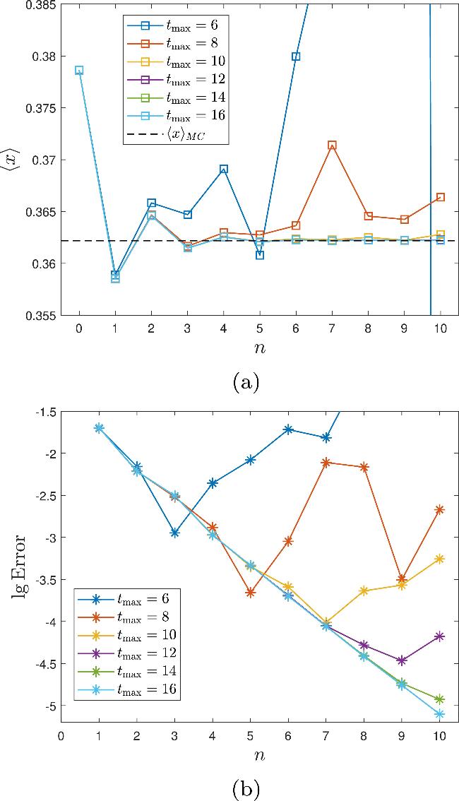
Figure 3. Numerical results and convergence rates of the layered scheme applied to the Feray-like system, shown for different truncation tmax. (a) The numerical results of ⟨x⟩ with different tmax. For different truncation tmax, there exists a threshold value $\hat{n}$ for the expansion order n. Within this threshold, the numerical results gradually converge to the exact value as the expansion order n increases. However, once the threshold is exceeded, the error increases with the increase of n. The black dashed line in the figure denotes the benchmark value ⟨x⟩MC obtained by the Monte Carlo method. (b) The convergence with different tmax. Within the threshold $\hat{n}$, the numerical results of the layered scheme exhibit an exponential convergence as the expansion order n increases. |
For comparison, we also computed the expectation value ⟨x⟩ using the induced map method, the direct cycle expansion, and the stability ordering. In intermittent systems, the presence of a vast number of long-period orbits with extremely small stability eigenvalues leads to extremely slow convergence for both the direct cycle expansion and the stability ordering, regardless of the chosen truncation length ${t}_{{\rm{\max }}}$, and they eventually converge to incorrect values. For the induced map method, once ${t}_{{\rm{\max }}}$ exceeds 10, its accuracy is primarily limited by the approximation degree nInd. Since the induced map method and the layered scheme involve different parameters, a direct comparison is not feasible. Instead, we compare them under approximately equivalent computational costs. When ${t}_{{\rm{\max }}}=10$ and nInd = 8, the induced map method converges to ⟨x⟩ ≈ 0.363 with an accuracy of about 10−2.5, slightly worse than the layered scheme (with ${t}_{{\rm{\max }}}=16$, n = 8), which achieves an accuracy of 10−4.5. Increasing nInd to 17 while keeping ${t}_{{\rm{\max }}}=10$ improves the result to ⟨x⟩ ≈ 0.3624 with accuracy 10−4.5, still slightly below the 10−5 accuracy attained by the layered scheme with ${t}_{{\rm{\max }}}=16$ and n = 10. Therefore, in intermittent systems the layered scheme significantly outperforms the other three approaches in both accuracy and computational efficiency.
Figures 4(a) and (b) benchmark our layered scheme against the conventional cycle expansion and the stability ordering scheme for a system with four singularities located at the endpoints of the phase interval and the period-2 orbit points as displayed above. To minimize unknown coefficients and enhance stability, we derived analytic relations between singular layer coefficients from equation (5 ):
$\begin{eqnarray}{c}_{{s}_{i}}=\left\{\begin{array}{ll}\frac{{a}^{2}{c}_{{s}_{i-1}}}{{\pi }^{2}(a-1+{x}_{{s}_{i-1}})},\quad & \,i=2,5\\ \frac{{a}^{2}{c}_{{s}_{i-1}}}{{\pi }^{2}(1-{x}_{{s}_{i-1}})},\quad & \,i=3,4,6\end{array}\right.,\end{eqnarray}$
where ${x}_{{s}_{i}}$ represents the sequence of singularities along the trajectory evolving from the first one at x = 1 (for i = 1), to the later ones at: ${x}_{{s}_{i}}=1,0,{x}_{a},{x}_{b},{x}_{a},{x}_{b}$, each having a specific ${c}_{{s}_{i}}$. Our approach achieves exponential accuracy with increasing tmax and reaches a accuracy level of 10−6 for ${t}_{\max }=12$, while traditional method and stability ordering shows algebraic convergence [figure 4(b)]. Moreover, it is evident that even with a relatively short truncation length, our scheme can attain a considerably higher numerical accuracy than existing methods. This indicates that, compared to the traditional cycle expansions, which only utilizes information from UPOs, the additional dynamical information introduced here plays an essential role.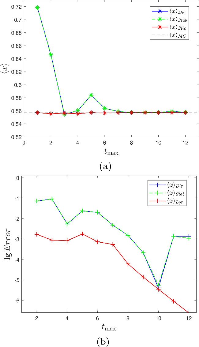
Figure 4. Comparison of numerical results and convergence rates for the four-singularity system f4s(x) across different schemes: the direct cycle expansion (blue solid lines), the stability ordering (green dashed lines) and the layered scheme. (a) The numerical results of direct cycle expansion (⟨x⟩Dir), stability ordering scheme (⟨x⟩Stab) and the layered scheme (⟨x⟩Lyr). At a relatively short tmax, the layered scheme can attain a considerably high accuracy. The black dashed line in the figure denotes the benchmark value ⟨x⟩MC obtained by the Monte Carlo method. (b) The convergence rates of the three schemes. ⟨x⟩Lyr converge much faster and steadily than the other schemes, reaching 10−6.6 at tmax = 12. |
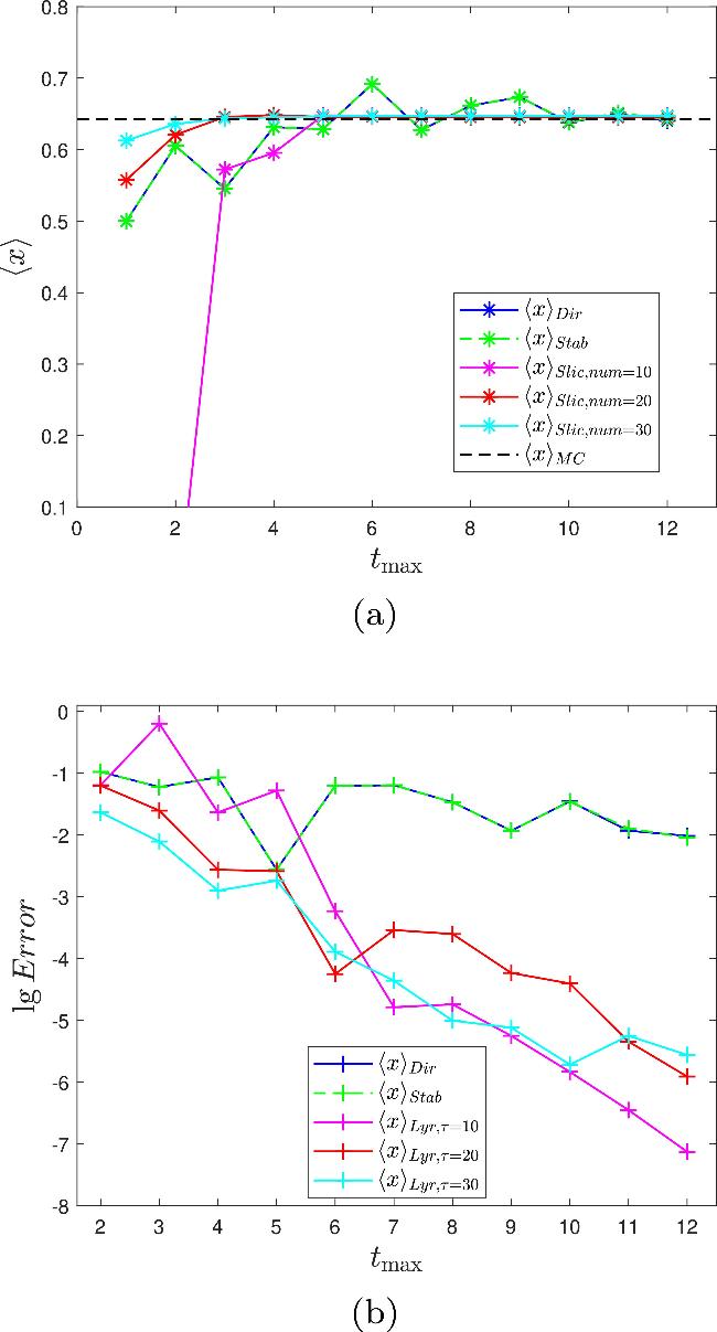
For a system with infinitely many singularities [see figure 5(a)], generated by iterating an initial singularity at ${x}_{r}=f(\frac{1}{2})$ through ${f}^{i}({x}_{r})\,(i\in {\mathbb{N}})$, all singular neighborhoods share the same singular exponent $-\frac{1}{2}$. These aperiodic points densely fill the accessible phase space ${ \mathcal M }=[f({x}_{r}),{x}_{r}]$ [see figure 5(b)]. While the measure decomposes into infinitely many singular layers plus a hyperbolic component, solving an infinite-rank equation is computationally intractable. We therefore exploit the self-similar structure of singularities to reduce degrees of freedom and implement recursive relations among the coefficients based on equation (5 ):
$\begin{eqnarray}{c}_{{s}_{i+1}}=\frac{{c}_{{s}_{i}}}{\sqrt{| {f}^{{\prime} }({x}_{{s}_{i}})| }},\quad i=1,2,3,...\end{eqnarray}$
where ${f}^{{\prime} }(x)=R-2Rx$ is the stability factor at each singularity of f(x). Besides, a finite truncation of the singularities seems reasonable since the asymptotic decay of singularity peaks upon iteration is clearly observed in figure 5(b), that is, higher-order singularities exhibit exponentially diminishing influence. We implement a simple τ-controlled truncation (here, τ denotes the number of singularities retained sequentially in the computation) and compare the average value ⟨x⟩ computed via a direct cycle expansion (⟨x⟩Dir), the stability ordering scheme (⟨x⟩Stab) and our layered approximation (⟨x⟩Lyr,τ) for τ = 10, 20, 30. figures 6(a) and (b) demonstrate our layered scheme's exponential efficiency. The results of the layered scheme ⟨x⟩Lyr,τ can attain a considerably high accuracy at a relatively short tmax. By combining the hyperbolic layer's cycle expansion—which supplies the baseline—with the singular layers that provide the necessary corrections, the layered approximation scheme achieves significantly faster convergence overall than other schemes. Furthermore, the truncation of singular layers has an important impact on the convergence. Figure 6(a) reveals that, for small truncation (tmax ≤ 5), the results obtained with τ = 30 are more accurate than those obtained with τ = 10 and τ = 20. Conversely, figure 6(b) shows that, as tmax grows, the convergence of τ = 10 seems to be more steady than that of τ = 30 and τ = 20. A key practical consideration is the trade-off between singularity resolution (large τ) and numerical stability. These trends signal that the retained number τ of singular layers should be tuned to the truncation tmax: at small tmax a larger τ enhances accuracy, whereas for larger tmax an excessive count of singular layers destabilizes the computation and degrades precision, possibly because of the kinks generated by including singular functions in the layered expansion. Practitioners can simply adopt τ = 20 as a robust default without noticeable loss of precision for different ${t}_{{\rm{\max }}}$, adjusting only when high precision at low truncation is required.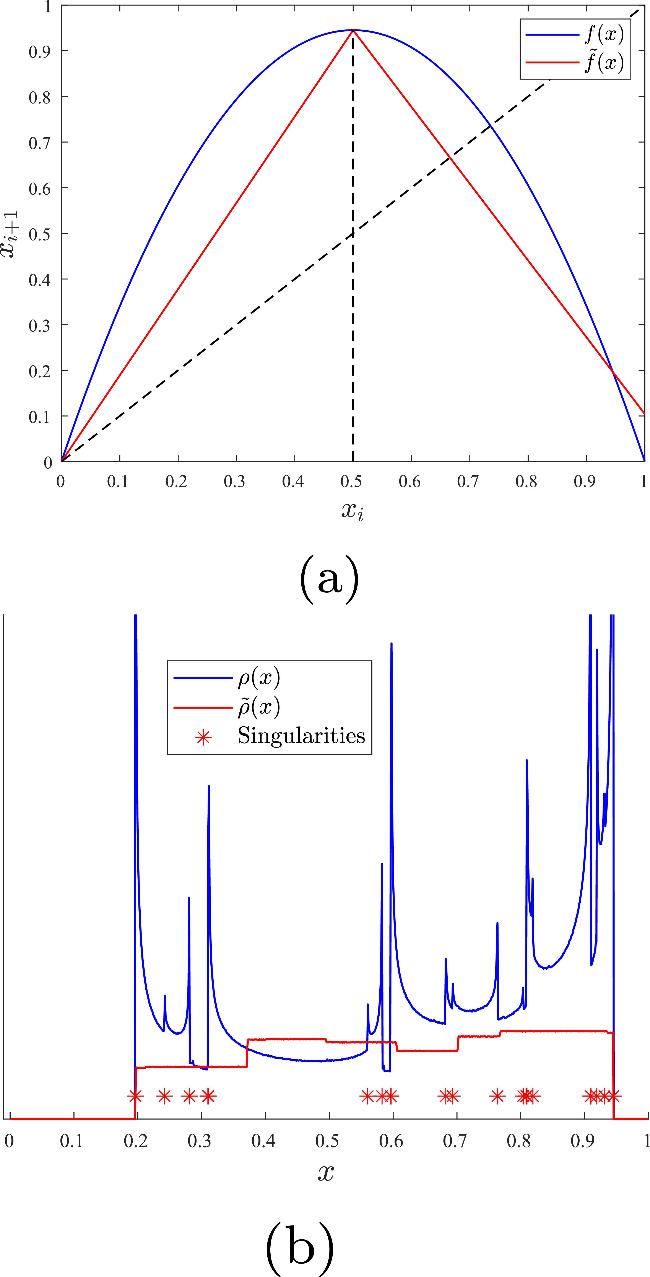
Figure 5. A system exhibiting a natural measure with infinite singularities. (a) The graph of the system f(x) = Rx(1 − x), R = 3.786… (blue solid line) and the conjugate map $\tilde{f}(x)$ (red solid line, non-unique). (b) The singular natural measure ρ(x) of f(x) and the hyperbolic natural measure $\tilde{\rho }(x)$ of $\tilde{f}(x)$. $\tilde{\rho }(x)$ cover the same phase space as ρ(x). The first 30 singularity peaks (red * marks the horizontal positions) densely sample the phase space and asymptotically decay with iteration order. |
Figure 6. Comparison of numerical results and convergence rates for the infinite-singularity system across different schemes: the direct cycle expansion (blue solid lines), the stability ordering (green dashed lines) and the layered scheme with different number of singularities retained (denoted by different τ). (a) The numerical results of direct cycle expansion (⟨x⟩Dir), stability ordering scheme (⟨x⟩Stab) and the layered scheme (⟨x⟩Lyr,τ) with τ = 10, 20, 30. The black dashed line in the figure denotes the benchmark value ⟨x⟩MC obtained by the Monte Carlo method. (b) The convergence rate of the three schemes. ⟨x⟩Lyr,τ converge much faster than the other schemes, reaching at least 10−6 accuracy at tmax = 12, whereas the other schemes remain below 10−2. |
4. Conclusions and discussions
The layered approximation scheme, combining additional dynamical information with cycle expansions, ensures rapid convergence and high computation accuracy, resolving the traditional accuracy and efficiency issues to some extent. Decomposing the natural measure into singular and hyperbolic layers clarifies how singularities influence the system's statistical properties, which may play important roles in the analysis of complex non-equilibrium systems. From the perspective of natural measure, the dynamical invariance condition provides extra corrections beyond the UPOs. This opens a promising path towards wider application of cycle expansions and high-precision computation for chaotic systems.
In this work, we employed the layered scheme to study dynamical systems with distinct singularity characteristics: (i) Intermittent systems, where the natural measure possesses a singularity at the origin; (ii) multi-singularity systems, where singularities arise both on periodic orbits and at phase-space boundaries; (iii) systems exhibiting infinitely many singularities in the natural measure. In these numerical examples, the numerical accuracy and convergence rate of the layered scheme are superior to those of existing schemes and hence relieve a few well-known limitations of traditional cycle expansions and existing schemes.
Nevertheless, the layered scheme still has its own limitations. How to achieve an elegant trade-off between numerical accuracy and stability within this method still calls for deeper investigation; at present we can only proceed by trial-and-error or empirical tuning. While the current work focuses on one-dimensional maps for clarity and benchmarking, its application to more complex systems still requires further investigation. The conceptual framework of decomposing the invariant measure into singular and hyperbolic components remains conceptually applicable. In higher dimensions, singularities often manifest on unstable manifolds or fractal basin boundaries [33, 34]. The challenge lies in analytically characterizing these complex singularity structures and constructing a suitable hyperbolic conjugate system. This is a promising direction for future work, potentially building on frameworks for cycle expansions in higher-dimensional systems [5, 35–37]. However, the convergence issues of cycle expansion have not yet been fully resolved, and balancing mathematical rigor with physical operability remains an open question. The Layered scheme may provide useful insights for the readers and offer a potential approach to tackling more realistic challenges in the future.
This work was supported by the National Natural Science Foundation of China (No. 12375030), by BUPT Excellent PhD Students Foundation (CX2023210), and also by the Key Program of National Natural Science Foundation of China (No. 92067202).