


1. Introduction
Synchronization is a fundamental mechanism through which collective behavior emerges in large assemblies of interacting dynamical units [1, 2]. It underlies coordinated activity in a wide range of natural and engineered systems, including neuronal populations, biological oscillators, power grids, and chemical or electronic circuits [3]. In such systems, synchronization reflects the spontaneous alignment of individual dynamics resulting from mutual interactions, and its onset is commonly described as a phase transition from incoherent to coherent motion.
Early studies established that network structure strongly affects the critical coupling required for synchronization, yet the transition itself was generally found to be continuous, even in highly heterogeneous networks such as scale-free topologies [4–6]. In this classical picture, synchronization emerges smoothly as the coupling strength increases, corresponding to a second-order phase transition. This view was later challenged by the discovery that abrupt, discontinuous transitions can occur when structural and dynamical properties are correlated [7]. In particular, it was shown that when the natural frequencies of Kuramoto oscillators are positively correlated with node degree in scale-free networks, the system undergoes a sudden jump from incoherence to global synchrony. This phenomenon, now known as explosive synchronization (ES), is characterized by bistability and the presence of hysteresis between forward and backward transitions in coupling strength [8].
The interest in ES grew rapidly following broader discoveries of abrupt phase transitions in complex systems, such as discontinuous percolation in random and heterogeneous networks [9, 10]. Such abrupt transitions are now recognized as widespread in natural and social systems and are often associated with critical risks or rapid systemic changes. Within the context of synchronization, ES has been widely investigated in previous research [11–14]. It has been reported in a variety of dynamical frameworks, including delayed Kuramoto models [15], second-order (inertial) oscillators [16, 17], networks of FitzHugh–Nagumo units [18], and chaotic oscillators [19]. Recently, Li et al [20] represented the emergence of two abrupt, first-order (explosive) transitions in both synchronization and cooperation in a unified model that couples collective synchronization with evolutionary game dynamics, where agents can either cooperate or defect. Dai et al [21] demonstrated that introducing a positive feedback between the coupling strength and the global order parameter in a high-dimensional Kuramoto model produces ES transitions in even dimensions and novel time-dependent rhythmic states in odd dimensions. Notably, experimental realizations of ES have been demonstrated using electronic circuits, confirming that explosive transitions are not merely theoretical constructs [22].
In recent years, increasing attention has been devoted to synchronization phenomena in temporal and adaptive networks, where interactions evolve dynamically and feedback on the collective state of the system [23–25]. More recent studies have revealed that ES can arise even in the absence of explicit structural–dynamical correlations, provided that interactions evolve in time. In adaptive networks, where coupling strengths depend on local or global coherence, feedback mechanisms can spontaneously generate the conditions required for abrupt transitions. Various adaptive schemes, ranging from anti-Hebbian rules to nonlinear feedback between coupling weights and order parameters, have been shown to induce bistability and hysteresis in oscillator networks [26–29]. These results highlight the importance of temporal interactions and adaptive processes in shaping collective dynamics. In addition to studies focused on the structural mechanisms of synchronization, recent work has explored how fluctuations in intrinsic dynamical parameters can induce abrupt transitions and rich collective behavior in complex networks. For example, Zhang et al [30] investigated coupled oscillators subject to damping fluctuations in small-world complex networks, deriving analytical conditions to demonstrate that the probability of achieving synchronization can undergo abrupt changes with respect to network size, coupling structure, and noise intensity. Furthermore, the researchers have shown that intrinsic parameter fluctuations provide an alternative route to complex synchronization phenomena beyond conventional monotonic transitions. For example, Meng et al [31] studied networks of oscillators with time-varying natural frequencies and derived asymptotic stability conditions for the mean field, demonstrating that both synchronization probability and the mean first synchronization time exhibit non-monotonic dependence on network heterogeneity and other parameters.
Despite these advances, comparatively less attention has been given to networks whose topology itself evolves over time. In temporal networks, connections between nodes may appear, disappear, or rewire on timescales comparable to the intrinsic dynamics. Such structural variability is a natural feature of many real systems, including social interactions, mobile communication networks, and biological contact patterns. Previous work has explored ES in temporal settings where oscillators move in space or randomly switch interaction partners [32]. These studies demonstrate that temporal connectivity can either suppress or enhance explosive behavior, depending on how rapidly and extensively the network changes.
In this work, we investigate ES in a distinct class of time-varying networks constructed through stochastic rewiring. Starting from an initial random graph, links are randomly replaced at each time interval with a prescribed probability, generating a dynamically evolving topology while preserving the mean degree. Here, randomness arises solely from the temporal rewiring of a single evolving network. For each parameter set, we begin from one Erdős–Rényi realization and allow the topology to change stochastically in time according to the defined rewiring rule. The oscillator dynamics are governed by the inertial Kuramoto model, which naturally incorporates a second-order time scale and is known to support ES. By systematically varying the rewiring probability, rewiring frequency, and network degree, we examine how temporal topology controls the nature of the synchronization transition and the associated hysteresis.
The remainder of the paper is organized as follows. Section 2 introduces the network construction and the dynamical model. Section 3 presents numerical results on synchronization transitions, bistability, and hysteresis across different parameter regimes. Finally, section 4 summarizes the main findings and discusses their implications for synchronization in temporal complex networks.
2. Model description
We consider a network of $N=100$ coupled phase oscillators whose internal dynamics follow the inertial extension of the Kuramoto model. Each oscillator $i$ is characterized by its phase ${\theta }_{i}(t)$ and angular velocity ${\dot{\theta }}_{i}(t)$. The intrinsic frequency ${\omega }_{i}$ is drawn independently from a prescribed distribution. The evolution equation is,
$\begin{eqnarray}m{\ddot{\theta }}_{i}+\gamma {\dot{\theta }}_{i}={\omega }_{i}+\frac{\lambda }{k}\displaystyle \sum _{j=1}^{N}{A}_{{ij}}\left(t\right)\sin \left({\theta }_{j}-{\theta }_{i}\right),\end{eqnarray}$
where $m$ denotes the inertial parameter, $\gamma $ is the damping coefficient, and $\lambda $ is the coupling strength. The adjacency matrix $A(t)=[{A}_{{ij}}(t)]$ encodes the instantaneous connectivity of the time-dependent network. The scalar $k$ is the average degree of the network and is used to normalize the effective interaction strength.2.1. Network construction
At the initial time, the network is generated as an undirected random graph with average degree $k$. Edges are assigned uniformly at random, ensuring a homogeneous connectivity profile across the ensemble. Each link represents a bidirectional interaction channel between a pair of oscillators. The connectivity pattern is allowed to vary as time evolves. At discrete time intervals of duration ${\rm{\Delta }}t$, each existing link is independently selected for stochastic rewiring. The quantity ${\rm{\Delta }}t$ therefore sets the characteristic timescale of topology updates. For convenience, we define the rewiring frequency $f=1/{\rm{\Delta }}t$, which measures how often the network structure is refreshed relative to the oscillator dynamics. Larger $f$ corresponds to more rapid topological switching. Specifically, every link is removed and replaced by a new randomly selected edge with probability ${P}_{{\rm{rewire}}}$.
Thus, ${P}_{{\rm{rewire}}}=0$ corresponds to a static network, whereas larger values of ${P}_{{\rm{rewire}}}$ lead to increasingly rapid fluctuations of the interaction topology. Figure 1 illustrates the construction of the time-varying random network used throughout this study. The initial configuration, labeled $T\unicode{8320}$, is a simple random graph with average degree $k$, where all links are fixed and drawn uniformly at random. At each subsequent time interval, the network undergoes stochastic rewiring: every existing link is independently selected for removal with probability ${P}_{{\rm{rewire}}}$. The links chosen for rewiring are highlighted in gray. For each removed link, a new edge is introduced between a randomly selected pair of previously unconnected nodes; these newly created connections are shown in dark red. This rewiring rule preserves the mean degree of the network while continuously altering its connectivity structure. As a result, the interaction topology evolves over time from ${T}_{0}$ to later snapshots ${T}_{1},{T}_{2},\ldots $ providing a controlled mechanism for studying synchronization under dynamic connectivity.
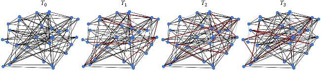
Figure 1. Schematic illustration of the random network with stochastic rewiring. Black links represent the initial network at time ${T}_{0}$. At each subsequent time step, existing links are selected for rewiring with probability ${p}_{{\rm{rewire}}}$; links scheduled for removal are shown in light gray. For each removed link, a new connection is added between a randomly chosen pair of nodes not previously connected, depicted in dark red. This process preserves the mean degree while generating a time-varying interaction topology, providing a controlled way to find the effect of temporal connectivity changes on synchronization dynamics. |
This simple mechanism generates a temporally switching random network in which oscillators interact through neighbors that change over time. As a result, the system interpolates between quenched heterogeneity and fast-mixing connectivity, depending on the value of ${P}_{{\rm{rewire}}}$.
2.2. Interpretation
The temporal rewiring implements a form of dynamic mixing that influences how oscillators exchange phase information. For small ${P}_{{\rm{rewire}}}$, oscillators interact repeatedly with nearly the same neighbors, preserving quenched disorder. As ${P}_{{\rm{rewire}}}$ increases, interactions average over a larger portion of the network, potentially facilitating synchronization through an effective homogenization of coupling pathways. The inertial term adds a second dynamical timescale, enabling rich transitions between incoherence and coherent motion shaped jointly by inertia, topology switching, and coupling strength.
2.3. Synchronization measure
To quantify the collective dynamics of the network, we employ the standard Kuramoto order parameter as a global indicator of phase coherence. At any time $t$, the order parameter is defined as
$\begin{eqnarray}R\left(t\right)=\left|\frac{1}{N}{\sum }_{j=1}^{N}{{\rm{e}}}^{{\rm{i}}{\theta }_{j}(t)}\right|.\end{eqnarray}$
The quantity $R(t)$ lies in the interval $[0,1]$. Values close to $0$ correspond to an incoherent distribution of phases, while $R(t){\rm{\approx }}1$ indicates near-perfect phase synchronization.
Because the network connectivity is time-varying, fluctuations in the collective state may occur even when the system is close to a coherent regime. Therefore, we compute the synchronization index as the temporal average, after discarding an initial transient of duration ${T}_{{\rm{trans}}}=100$, over a time window ${T}_{{\rm{avg}}}=900$. The quantity $R$ provides a robust scalar measure of global synchrony in the presence of stochastic rewiring, inertia, and heterogeneous intrinsic frequencies.
3. Results
Numerical integration of equations (1 )–(2 ) is performed using a fourth-order Runge–Kutta scheme with fixed time step, and all oscillators are initialized with randomly sampled phases and velocities. The parameters of the systems are fixed at $m=1$ and $\gamma =0.3$, while ${\omega }_{i}$ are drawn from a Gaussian distribution with mean ${\omega }_{{\rm{mean}}}=0$ and standard deviation ${\omega }_{{\rm{std}}}=0.2$. For each realization, we vary the coupling strength $\lambda $ quasistatically in two directions: (i) a forward continuation, in which $\lambda $ is gradually increased from zero, and (ii) a backward continuation, in which the system is initialized in the synchronized regime and $\lambda $ is slowly decreased. At each step, the instantaneous order parameter $R(t)$ is evaluated and subsequently time-averaged to obtain $R$.
To establish a baseline for the influence of temporal rewiring, we first examine the behavior of the system on static networks. We specifically analyze two representative random networks: one with average degree $k=16$, corresponding to a moderately sparse topology, and another with $k=40$, representing a substantially denser network. These two cases allow us to contrast how the underlying connectivity influences the onset and structure of synchronization transitions.
Figure 2 summarizes the behavior of the order parameter for both networks in the static (non-rewired) setting. Panels (a) and (b) correspond to $k=16$ and $k=40$, respectively. In each panel, the dark blue curve denotes the forward continuation, whereas the light blue curve represents the backward sweep of the coupling strength. In both cases, the system exhibits an explosive transition to synchronization. As $\lambda $ increases, the order parameter remains small for a broad parameter interval and then undergoes an abrupt jump to a value close to unity. The backward continuation follows a distinct branch, revealing a pronounced hysteresis loop and confirming the presence of bistability between incoherent and synchronized states. While ES occurs in both networks, the magnitude of the discontinuity differs markedly. The jump in R is larger in the sparser network with $k=16$, indicating a sharper transition. In contrast, the network with $k=40$ exhibits a smaller but still significant discontinuity. This suggests that denser connectivity tends to smooth the synchronization boundary, reducing the severity of the abrupt onset while preserving the hysteretic nature of the transition.
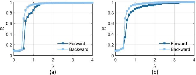
Figure 2. Forward (dark blue) and backward (light blue) synchronization transitions in static random networks with $N=100$ oscillators. Panel (a) shows the order parameter curves for a network with mean degree $k=16$, while panel (b) corresponds to a denser network with $k=40$. In both cases, increasing and decreasing the coupling strength reveal the characteristic hysteresis loop associated with explosive synchronization. The discontinuous jumps and separated branches confirm bistability and demonstrate that explosive synchronization already exists in the static baseline networks. |
We first analyze the network with average degree $k=16$ and examine how synchronization depends on the interplay between the coupling strength $\lambda $, the rewiring probability prewire, and the rewiring frequency f. Figure 3 displays a two-dimensional map of the forward order parameter $R$ in the ($f,\lambda $) plane for six values of prewire: panels (a)–(f) correspond to ${p}_{\mathrm{rewire}}=0.01,{\rm{}}0.05,{\rm{}}0.1,{\rm{}}0.2,{\rm{}}0.3,\,0.4$ respectively. The rewiring frequency is shown on a logarithmic scale for better visualization across several orders of magnitude. Dark red shades indicate low coherence (asynchrony), whereas dark blue denotes complete synchronization. The presence of a sharp transition from red to blue reflects an explosive (abrupt) onset of synchrony, while the appearance of intermediate colors corresponds to a continuous, second-order–like transition.
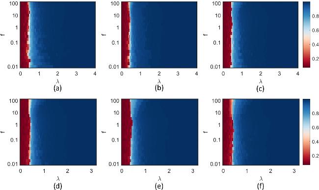
Figure 3. Two-dimensional map of the forward order parameter $R$ for the network with mean degree $k=16$, shown in the $(f,\lambda )$ plane for six rewiring probabilities. Panels (a)–(f) correspond to ${p}_{\mathrm{rewire}}=0.01,0.05,0.1,\,0.2,\,0.3,\,0.4$, respectively. The rewiring frequency $f$ is plotted on a logarithmic scale to highlight behavior across multiple time scales. Dark red indicates low coherence (asynchronization), while dark blue denotes full synchronization, with intermediate colors representing partial coherence. The maps show that increasing rewiring probability and switching frequency progressively favors abrupt, explosive transitions over smooth continuous ones. |
Across all panels, the critical coupling strength required for synchronization remains broadly similar as $f$ varies, and only slight shifts are observed, indicating that the rewiring frequency moderately influences but does not dominate the transition threshold. For the smallest rewiring probability, ${p}_{{\rm{rewire}}}=0.01$ [panel (a)], all transitions are continuous, with a smooth progression from low to high $R$. When ${p}_{\mathrm{rewire}}=0.05$ [panel (b)], ES appears only within a narrow band of frequencies, specifically around f ≈ 0.0125 and f ≈ 0. At intermediate rewiring probabilities, more diverse behavior emerges. For ${p}_{{\rm{rewire}}}=0.1$ [panel (c)], explosive transitions occur for several widely separated frequency values, including high-frequency regimes such as $f=100,\,50,\,20$ and low-frequency points around $f=0.015$ and $f=0.011$. For larger values of ${p}_{{\rm{rewire}}}$ (panels (d), (e), corresponding to $0.2,\,0.3$), ES becomes prominent for sufficiently large rewiring frequencies, with sharp transitions appearing consistently whenever $f\gtrsim 2.5$. In these regimes, rapid topological switching combined with frequent rewiring appears to enhance the nonlinearity of the transition and promote bistability. Finally, in panel (f) where ${p}_{{\rm{rewire}}}=0.4$, the sharp jump in the order parameter $R$ value and also a small hysteresis can be found for all frequencies, hence, the ES can be found. Generally, the results show that continuous transitions dominate when the network is rewired infrequently or with small probability, whereas ES becomes increasingly likely as both prewire and $f$ grow, culminating in sharp transitions in the high-frequency, high-probability regime.
Figure 4 presents the forward and backward continuation of the order parameter $R$ for the $k=16$ network under temporal rewiring. We examine four representative rewiring probabilities, ${p}_{{\rm{rewire}}}=0.01,{\rm{}}0.05,{\rm{}}0.1$ and $0.4$, shown in panels (a)–(d), respectively. Each panel contains three subplots corresponding to different rewiring frequencies: fast-switching ($f=50$, left), intermediate switching ($f=2.5$, middle), and slow switching ($f=0.025$, right). For the smallest rewiring probability, ${p}_{{\rm{rewire}}}=0.01$ [panel (a)], no ES is observed for any of the switching frequencies. The forward and backward curves nearly coincide, yielding smooth and continuous transitions between incoherent and synchronized regimes. When the rewiring probability increases to ${p}_{{\rm{rewire}}}=0.05$ [panel (b)], an explosive transition emerges only in the slow switching case ($f=0.025$). In this regime, the forward and backward branches separate slightly, producing a small hysteresis loop that indicates weak bistability. For medium and fast-switching, although the transitions have some jumps, there is no hysteresis between branches.
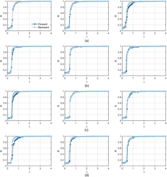
Figure 4. Forward and backward $R$ parameters for the network with $k=16,$ shown for three switching frequencies: $f=50$ (left), $f=2.5$ (middle), and $f=0.025$ (right). Panels correspond to different values of the rewiring probability: (a) ${p}_{{\rm{rewire}}\,}=0.01$, (b) ${p}_{{\rm{rewire}}\,}=0.05$, (c) ${p}_{{\rm{rewire}}\,}=0.1$, and (d) ${p}_{{\rm{rewire}}\,}=0.4$. The separation between forward and backward branches illustrates how explosive synchronization emerges only for specific combinations of rewiring probability and switching frequency. |
A different trend appears for larger rewiring probabilities. When ${p}_{{\rm{rewire}}}=0.1$ [panels (c)], ES is observed only in the fast-switching case ($f=50$). In these cases, the abrupt jump between low and high $R$ is visible, but the hysteresis region, representing the difference between forward and backward transitions, is relatively narrow, indicating that the bistable window is small. For intermediate switching although the jump exists, there is no hysteresis and in slow switching, the transitions again revert to a smooth and continuous form. Finally, for larger probabilities, as in panel (d), in which ${p}_{{\rm{rewire}}}=0.4$, the hysteresis exists in all cases of slow, intermediate and fast-switching. In summary, these results show that the appearance of ES depends sensitively on the interplay between the rewiring probability and the switching frequency. Low probabilities favor continuous transitions, moderate probabilities produce ES only under slow switching, and higher probabilities form ES in all frequencies, albeit with minimal hysteresis.
To further illustrate the bistability underlying the explosive transition, figure 5 presents the spatiotemporal dynamics of the system for rewiring probability ${p}_{{\rm{rewire}}\,}=0.1$, where ES was observed. The figure displays the local order parameter ${R}_{L}$, computed for each oscillator using only its four nearest neighbors in the instantaneous network, thereby allowing us to visualize spatial coherence at a local scale. The top row (panels a–c) corresponds to the forward continuation, where the coupling strength is increased gradually. Results are shown for $\lambda =0.45,\,0.5$, and $0.55$. In panels (a) and (b), the system remains fully asynchronous: the spatiotemporal patterns exhibit irregular fluctuations with low ${R}_{L}\,$ values, indicating the absence of local phase alignment. When the coupling strength reaches $\lambda =0.55$ [panel (c)], the system undergoes a sudden transition; $R$ jumps abruptly to a high value, and the network shifts into a more ordered state. Distinct coherent clusters begin to form across the network, characterized by regions where ${R}_{L}{\rm{\approx }}1$, signifying local synchrony. This sudden appearance of coherent structures highlights the sharpness of the explosive transition.
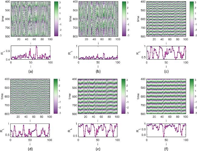
Figure 5. Spatiotemporal dynamics of the network and the corresponding local order parameter (${R}_{L}\,$) for $k=16$ and ${p}_{{\rm{rewire}}\,}=0.1$, shown for forward transitions (first row) and backward transitions (second row). Panels correspond to different coupling strengths: (a), (d) $\lambda =0.45$, (b), (e) $\lambda =0.5$, and (c), (f) $\lambda =0.55$. The figure highlights how the network dynamics and local synchronization evolve with varying $\lambda $ during forward and backward transitions. These spatiotemporal dynamics provide a direct visual signature of bistability and hysteresis underlying explosive synchronization. |
The bottom row (panels d–f) displays the corresponding backward continuation, where the coupling strength is decreased from the synchronized state. Even at relatively low values of $\lambda $ (panel d), the network retains several coherent clusters, indicating that phase alignment persists longer during the backward sweep. Therefore, as $\lambda $ is further reduced coherent groups remain visible and the system gradually approaches incoherence. Compared to the forward continuation, the backward dynamics show a clearly smoother desynchronization process, with consistently larger values of the global order parameter and the presence of localized coherent domains even at coupling strengths where the forward branch was fully asynchronous. These contrasting behaviors between forward and backward transitions provide direct evidence of bistability: the system supports both coherent and incoherent states over the same range of coupling strengths, and the resulting hysteresis is reflected in the markedly different spatiotemporal patterns.
To assess how network density influences the emergence of ES, we repeat the analysis for a denser random network with mean degree $k=40$. Figure 6 shows the forward order parameter $R$ in the ($f,\lambda $) plane for six different rewiring probabilities: panels (a)–(f) correspond to ${p}_{{\rm{rewire}}}=0.01,{\rm{}}0.05,{\rm{}}0.1,{\rm{}}0.2,{\rm{}}0.3$, and $0.4$, respectively. For the smallest rewiring probability, ${p}_{{\rm{rewire}}}=0.01$ [panel (a)], the transition from asynchrony to synchrony remains completely continuous across all switching frequencies. In contrast to the sparser network ($k=16$), where some explosive behavior still appeared for particular parameter combinations, the larger connectivity here effectively smooths the transition.
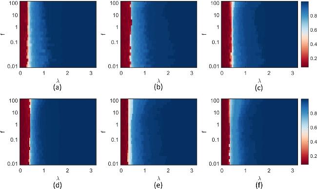
Figure 6. Two-dimensional map of the forward order parameter $R$ for the network with mean degree $k=40$, shown in the $(f,\lambda )$ plane for six rewiring probabilities. Panels (a)–(f) correspond to ${p}_{\mathrm{rewire}}=0.01,{\rm{}}0.05,{\rm{}}0.1,\,0.2,\,0.3,\,0.4$, respectively. The rewiring frequency $f$ is plotted on a logarithmic scale to highlight behavior across multiple time scales. Dark red indicates low coherence (asynchronization), while dark blue denotes full synchronization, with intermediate colors representing partial coherence. This figure demonstrates that dense connectivity enhances the robustness of abrupt transitions. |
When the rewiring probability increases to ${p}_{{\rm{rewire}}}\,=0.05$, $0.1$, and $0.2$ [panels (b)–(d)], ES becomes prevalent. In these cases, an abrupt transition is visible almost uniformly throughout the entire frequency range, from fast to slow switching. This indicates that for intermediate rewiring probabilities, the denser network robustly supports bistable dynamics and sharp jumps in the order parameter. For ${p}_{{\rm{rewire}}}=0.3$ [panel (e)], ES persists, but the magnitude of the jump in $R$ decreases, and the hysteresis becomes less pronounced, especially at higher switching frequencies. The transitions remain relatively sharp at low and intermediate frequencies, but the bistable region weakens as $f$ increases. At the highest rewiring probability, ${p}_{{\rm{rewire}}}\,=0.4$ [panel (f)], explosive transitions occur across all frequencies, yet the hysteresis width is noticeably smaller than in the strong explosive regime observed at ${p}_{{\rm{rewire}}}=0.2$. Thus, although high rewiring probability still supports abrupt transitions, the strong disorder introduced by frequent link replacement reduces the stability of the synchronized branch and narrows the bistable interval. In compared to the $k=16$ network, the denser $k=40$ network displays ES much more consistently across parameter space. Dense connectivity enhances the system's susceptibility to abrupt collective ordering, although very high rewiring probability can diminish the associated hysteresis.
To illustrate the qualitative differences between continuous and ES in the denser network, figure 7 presents examples of forward and backward order-parameter curves for three representative switching frequencies: fast-switching ($f=50$, left column), intermediate switching ($f=2.5$, middle column), and slow switching ($f=0.025$, right column). Results are shown for three rewiring probabilities: ${p}_{\mathrm{rewire}}=0.01,\,0.2$ and $0.4$, corresponding to panels (a)–(c), respectively. For the smallest rewiring probability, ${p}_{{\rm{rewire}}}=0.01\,$[panel (a)], all transitions remain fully continuous across the entire range of switching frequencies. This confirms that dense connectivity combined with weak rewiring effectively suppresses explosive behavior.
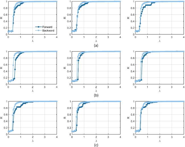
Figure 7. Forward and backward $R$ parameters for the network with $k=40,$ shown for three switching frequencies: $f=50$ (left), $f=2.5$ (middle), and $f=0.025$ (right). Panels correspond to different values of the rewiring probability: (a) ${p}_{{\rm{rewire}}\,}=0.01$, (b) ${p}_{{\rm{rewire}}\,}=0.2$, (c) ${p}_{{\rm{rewire}}\,}=0.4$. The pronounced hysteresis loops at intermediate rewiring probabilities indicate the strongest explosive behavior, while weak or strong rewiring reduces the bistable region. |
When the rewiring probability is increased to ${p}_{{\rm{rewire}}}=0.2$ [panel (b)], the nature of the transition changes dramatically. For all three switching frequencies, the order parameter exhibits a sudden jump as the coupling strength increases, clearly signaling ES. The backward curves follow a distinctly different branch, creating a wide hysteresis loop that indicates strong bistability. This regime constitutes the most robust and pronounced explosive behavior among the examined probabilities.
For the highest rewiring probability, ${p}_{{\rm{rewire}}}=0.4$ [panel (c)], the transitions remain explosive across all switching frequencies; however, the hysteresis region becomes noticeably narrower compared to the ${p}_{{\rm{rewire}}}=0.2$ case. Although abrupt jumps are still present, the difference between the forward and backward branches is reduced, indicating that frequent rewiring weakens the stability of the synchronized state and reduces the width of the bistable interval.
To systematically examine the role of network topology in shaping synchronization transitions, we extend our analysis to random networks with mean degree ranging from $k=5$ to $k=60$. For each network, we compute the forward and backward order parameters for three representative rewiring probabilities, ${p}_{\mathrm{rewire}}=0.01,\,0.1$, and $0.3$, and explore four switching frequencies, $f=20,{\rm{}}1,{\rm{}}0.1$ and $0.01$. Figure 8 presents the resulting two-dimensional diagrams of the synchronized state in the ($k,\lambda $) plane, where each row corresponds to a different rewiring probability and each column corresponds to a different switching frequency. Dark red indicates incoherence, dark blue denotes full synchrony, and intermediate colors represent partial coherence. Across all conditions, we observe that the onset of synchronization shifts to lower coupling strengths as the mean degree increases, consistent with the intuitive notion that denser connectivity facilitates collective coherence. For ${p}_{{\rm{rewire}}}=0.01$ (top row), ES appears predominantly at high switching frequency ($f=20$) and for small values of $k$. As $k$ increases, the explosive character gradually disappears, giving way to continuous transitions. At lower switching frequencies, explosive transitions become rarer; for example, at $f=0.1$ and $f=0.01$, the transitions are predominantly continuous across nearly all degrees.
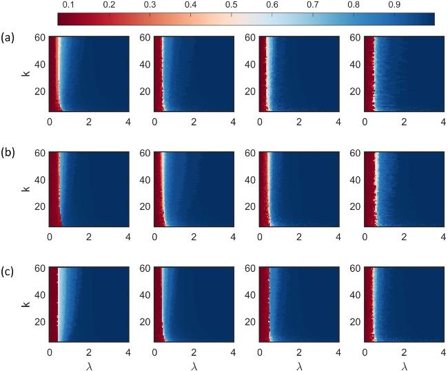
Figure 8. Two-dimensional map of the forward order parameter $R$ in the ($k,\lambda $) plane for the network, shown for four rewiring frequencies from left to right: $f=20,\,1,\,0.1$, and $0.01$. Panels (a)–(c) correspond to different rewiring probabilities: ${p}_{\mathrm{rewire}}=0.01,\,0.1$, and $0.3$, respectively. These diagrams summarize how network density and temporal rewiring jointly determine whether synchronization is continuous or explosive across parameter space. |
For the intermediate rewiring probability ${p}_{{\rm{rewire}}}=0.1$ (middle row), ES persists at high switching frequency ($f=20$) across a broader range of degrees. However, explosive behavior largely vanishes at $f=1$ and $f=0.1$, with transitions becoming fully continuous. At very slow switching ($f=0.01$), ES reappears but only for small $k$, indicating that sparse networks combined with slow rewiring can still support bistable transitions.
For the largest rewiring probability ${p}_{{\rm{rewire}}}=0.3$ (bottom row), ES occurs far more frequently than in the previous cases. At $f=20$ and $f=1$, explosive behavior is consistently observed for all degrees, although the corresponding hysteresis becomes noticeably smaller at $f=1$. As switching slows to $f=0.1$ and $f=0.01$, explosive transitions weaken; the hysteresis region shrinks, and for large degrees the transitions revert to continuous behavior.
Figure 9 summarizes these observations quantitatively by plotting the hysteresis area as a function of the mean degree for the same set of parameters. For ${p}_{{\rm{rewire}}}=0.01$ (top row), ES at $f=20$ occurs only for small degrees and fades as $k$ increases; at slower switching frequencies, hysteresis becomes minimal or absent. For ${p}_{{\rm{rewire}}}\,=0.1$ (middle row), hysteresis is present only at high switching frequency and small degree, consistent with the corresponding ($k,\lambda $) diagrams. For ${p}_{{\rm{rewire}}}\,=0.3$ (bottom row), hysteresis is broad for $f=20$ and persists for all degrees; at $f=1$ it remains present but reduced in size, and for $f=0.1$ or $0.01$ hysteresis shrinks and may vanish at larger degrees.
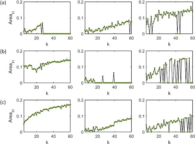


Figure 9. Hysteresis area between forward and backward transitions as a function of mean node degree $k$, shown for three rewiring frequencies from left to right: $f=20,1$, and $0.01$. Panels (a)–(c) correspond to different rewiring probabilities: ${p}_{\mathrm{rewire}}=0.01,0.1,$ and $0.3$, respectively. The variation of the hysteresis area quantitatively measures the strength of explosive synchronization and confirms that bistability is maximized for intermediate-to-high rewiring and rapid switching. |
4. Discussion
In this study, we examined how networks of inertial Kuramoto oscillators connected by time-varying random topologies develop ES. Compared with studies that focus solely on ensemble variability in static random networks [33], our work emphasizes temporal randomness arising from continuous random rewiring. This distinction allows us to isolate how time-dependent connectivity, controls the emergence of ES. By systematically varying the coupling strength, rewiring probability, switching frequency, and mean degree, we uncovered a rich interplay between dynamical and structural parameters that governs both the onset and the nature of the synchronization transition. Temporal restructuring can drastically modify the character of the transition, causing it to switch between continuous and explosive forms.
For the sparse network ($k=16$), only under particular rewiring probability and switching frequency combinations did ES appear. Low rewiring probability (${p}_{{\rm{rewire}}}=0.01$) produced smooth transitions across all frequencies, while intermediate values produced ES at either slow or fast-switching depending on the regime. Explosive transitions at high switching frequencies were favored by high rewiring probability, although the corresponding hysteresis was still minimal. These findings demonstrate that in sparse systems, the rapid creation and destruction of links can induce sudden ordering, but the bistable region is often narrow and sensitive to dynamical timescales.
In contrast, ES was far more robust in the denser network ($k=40$). Nearly all switching frequency experienced ES for intermediate rewiring probabilities (${p}_{\mathrm{rewire}}=0.05-0.2$), with significant hysteresis suggesting considerable bistability. The transition became smooth or the hysteresis dramatically decreased only for extremely low or extremely high rewiring probability. This implies that greater connectivity promotes more noticeable discontinuities in the transition to synchronization by improving the system's ability to maintain coherent clusters even in the face of dynamic perturbations.
This broader exploration across degrees and rewiring conditions confirms that topology and temporal variability jointly shape synchronization behavior. At very low rewiring probability, explosive transitions are mainly confined to sparse networks and fast-switching, while increasing the degree progressively smooths the transition. At intermediate probabilities, ES is most prominent under rapid switching but weakens as the network evolves more slowly. At high rewiring probability, explosive behavior becomes widespread but the hysteresis region typically shrinks, especially for slow switching. Together, these trends demonstrate that both connectivity and switching timescales determine whether bistability is sustained or suppressed.
Beyond the numerical characterization, these behaviors can be understood through the underlying physical mechanisms. Two competing ingredients dominate the dynamics: inertia, which introduces memory and enables multistability, and temporal rewiring, which continuously reshuffles neighbors and controls the effective mixing of the network. The balance between structural memory and dynamical mixing determines whether the transition is abrupt or continuous.
In static or slowly varying networks, oscillators repeatedly interact with nearly the same neighbors, creating quenched heterogeneity. Inertia then promotes the formation of metastable frequency clusters that persist over time. The coexistence of coherent and incoherent states produces bistability and hysteresis, leading to abrupt synchronization once the coupling crosses a threshold. By contrast, rapid rewiring homogenizes interactions. When links change faster than the intrinsic relaxation time of the oscillators, each node effectively samples many partners, approaching an annealed or mean-field regime. This enhanced mixing disrupts local correlations and destabilizes coherent clusters, smoothing the transition and reducing hysteresis.
ES is therefore strongest in intermediate regimes where structural memory and temporal mixing compete. Moderate-to-high rewiring probabilities allow coherent groups to form while still generating strong fluctuations, which enhances nonlinear feedback between local synchronization and coupling and maximizes bistability. If rewiring becomes too frequent, however, synchronized states lose stability and the explosive character weakens. This competition provides a unified explanation for both the emergence and the extinction of ES across parameter space.
The mechanisms observed here differ in key ways from those identified in static and adaptive networks. In static networks, ES is typically associated with quenched structural–dynamical correlations, such as degree–frequency matching or inertia-induced multistability, which create persistent heterogeneity and favor the coexistence of synchronized and incoherent states. In such cases, the abrupt transition is primarily determined by fixed topological disorder or imposed correlations that remain constant in time. Adaptive networks, on the other hand, generate explosive behavior through explicit feedback between dynamics and connectivity. There, coupling strengths or links evolve according to the instantaneous level of synchronization, effectively reinforcing coherent groups and suppressing incoherent ones. This feedback mechanism dynamically creates the bistability required for hysteresis and discontinuous transitions.
The temporally rewired networks studied here represent a distinct mechanism. In contrast to static networks, no permanent structural correlations are imposed, and unlike adaptive networks, no state-dependent feedback is introduced. Instead, ES emerges purely from the competition between inertia and stochastic topological switching. Rewiring controls the lifetime of interaction patterns and thus tunes the balance between structural memory and dynamical mixing. This mechanism shows that abrupt synchronization can arise even in the absence of designed correlations or adaptive rules, highlighting temporal variability itself as a fundamental control parameter for ES.
5. Conclusion
In summary, we have shown that temporal connectivity is not merely a perturbation to static synchronization dynamics but a key control parameter governing the nature of the transition. Depending on the rewiring probability, switching frequency, and network density, temporal networks may exhibit robust ES, weak bistability, or entirely continuous behavior.
Our results identify the parameter regimes where ES is strongest, where it is fragile, and where it disappears altogether. These findings highlight how the interplay between inertia, structural randomness, and network evolution shapes abrupt collective behavior, and they provide a general framework for understanding synchronization phenomena in realistic time-varying networks.
In the present work, we have focused specifically on the nature of the synchronization transition, continuous versus explosive, and the associated bistability induced by temporal rewiring. While variations of rewiring probability and switching frequency primarily modulate the abruptness and hysteresis of the transition, a systematic exploration of possible non-monotonic responses of order parameters to network or dynamical parameters lies beyond the current scope and will be an interesting direction for future investigation. Also, a fully analytical description of the observed ES transitions remains challenging for the present system. Traditional theoretical approaches to synchronization, typically rely on either static network structures or fast-annealed connectivity, where temporal fluctuations can be averaged out. The considered effects in this work violate the assumptions underlying standard analytical treatments, making it difficult to derive closed-form predictions for critical coupling strengths or hysteresis widths. Consequently, our study presented a systematic numerical exploration, and a detailed theoretical analysis will be pursued in future studies.