


1. Introduction
Across mechanics, physics, engineering and more, numerous nonlinear models yield partial differential equations with the time coordinate ‘t', which are nonlinear evolution equations (NLEEs). They excel in describing complex dynamic systems and nonlinear phenomena, which are vital in mathematical physics theoretical research and real-world scientific engineering applications, thus drawing broad attention from researchers and practitioners [1–7].
As a significant nonlinear evolution equation, the Kadomtsev–Petviashvili (KP) equation possesses a unique value in characterizing nonlinear wave phenomena. It is given as follows:
$\begin{eqnarray}{({u}_{t}+6u{u}_{x}+{u}_{xxx})}_{x}+\sigma {u}_{yy}=0,\end{eqnarray}$
where σ = ± 1 and u(x, y, t) is a function of the spatial variables x, y and the temporal variable t with subscripts representing its partial derivatives [8]. It enables accurate descriptions of long-wave motions under weakly nonlinear conditions in two-dimensional space that are widely observed in various physical contexts [9–11].Based on the KP equation, Akinyemi proposed a new (2+1)-dimension nonlinear evolution equation, which reads as 2 ) to the following (3+1)-dimension equation: 3 ) serves as a useful model for the dynamics of wave propagation in oceans, holding substantial promise for areas such as fluid mechanics, plasma physics, and other relevant disciplines [14, 16, 17].
$\begin{eqnarray}A{u}_{xt}+a{u}_{xx}+b{({u}^{2})}_{xx}+c{u}_{xxxx}+d{u}_{yy}=0,\end{eqnarray}$
where a, b, c and d are arbitrary real constants [12]. It offers an account of how waves with small amplitude and long characteristic wavelength propagate through a medium [13, 14]. Wazwaz extended equation ( $\begin{eqnarray}\begin{array}{l}{u}_{xt}+a{u}_{xx}+b{({u}^{2})}_{xx}+c{u}_{xxxx}+d{u}_{yy}\\ \,+\,\alpha {u}_{xy}+\beta {u}_{xz}+\gamma {u}_{yz}+\delta {u}_{zz}=0,\end{array}\end{eqnarray}$
where u(x, y, z, t) is a real function of x, y, z, t and the coefficients a, b, c, d, α, β, γ and δ are arbitrary real constants [15]. Equation (Researchers have dedicated substantial efforts to the exploration of equation (3 ) because of its significance in areas of fluid mechanics and plasma physics. Multiple soliton solutions and lump solutions were obtained by the Hirota bilinear method, together with periodic solutions, singular solutions, and many other physical nonlinear structures [15]. The sub-equation approach and the Sardar sub-equation approach were used to explore bright, dark, and combined dark-bright solutions [18]. The $({G}^{{\prime} }/G)$-expansion method was employed to acquire a rich set of exact solutions [17]. In [19], an array of mathematical functions were derived, including trigonometric, hyperbolic, and exponential functions. Integrability, rogue wave, lump-multi-stripe, and lump-multi-soliton solutions were discussed [14]. Y-shaped soliton solutions and various types of hybrid localized wave were also derived in [16]. In addition, Lie symmetries, bifurcation analysis, auto-Bäcklund and Cole–Hopf transformations, Lax pairs, space-time structure of the fusion/fission wave, and dynamical evolutions of molecules were also discussed [20–24].
When media exhibits uneven properties or boundaries take on irregular shapes, variable-coefficient models offer a truer portrayal of such situations, which are much more precise than models that rely on constant coefficients [25, 26]. In this paper, we would like to focus on a (3+1)-dimensional variable-coefficient nonlinear evolution equation based on equation (3 ), which is written as 4 ) provides insights into fluid mechanics and plasma physics. In our understanding, equation (4 ) has received very little attention.
$\begin{eqnarray}\begin{array}{l}{u}_{xt}+a(t){u}_{xx}+b(t){({u}^{2})}_{xx}+c(t){u}_{xxxx}+d(t){u}_{yy}\\ \,+\,\alpha (t){u}_{xy}+\beta (t){u}_{xz}+\gamma (t){u}_{yz}+\delta (t){u}_{zz}=0,\end{array}\end{eqnarray}$
where a(t), b(t), c(t), d(t), α(t), β(t), γ(t) and δ(t) are all real differentiable functions of t. By capturing the propagation of waves through non-uniform ocean media, equation (This paper is structured as follows. Section 2 focuses on applying the Weiss, Tabor and Carnevale (WTC) test to equation (4 ) for Painlevé analysis and obtaining the bilinear form of the equation by the Hirota bilinear method. In section 3 , X-shaped and Y-shaped soliton solutions will be derived through the soliton theory. The lump solution, breather solution and different interaction solutions, together with their propagation characteristics will be presented in section 4 . Various other types of solution will be given in section 5 . Finally, conclusions will be presented.
2. Painlevé integrability and bilinear form
2.1. Painlevé integrability
Grasping the solution structure of a specific nonlinear evolution equation (NLEE) hinges on Painlevé integrability, which plays an indispensable role in the process [27–29]. If solutions of a partial differential equation remain single-valued in the vicinity of non-characteristic movable singularity manifolds, the equation is considered to have the Painlevé property [30–32].
The WTC method with the simplified form of Krustal is applied to equation (4 ) for Painlevé analysis. Suppose that the solution of equation (4 ) can be expressed in the form of a generalized Laurent series expansion:
$\begin{eqnarray}\begin{array}{l}u(x,y,z,t)\\ ={\phi }^{p}(x,y,z,t)\displaystyle \sum _{j=0}^{\infty }{u}_{j}(x,y,z,t){\phi }^{j}(x,y,z,t),\end{array}\end{eqnarray}$
where φ(x, y, z, t) = x + ψ(y, z, t), ψ(y, z, t) is an arbitrary function of y,z and t, and uj(y, z, t), (j = 0, 1, 2, ⋯ ) are both analytic functions of y, z and t in the neighborhood of a non-characteristic movable singularity manifold defined by φ(x, y, z, t) = 0.We analyze the leading-order behavior. By inserting equation (5 ) into equation (4 ), we can get
$\begin{eqnarray*}p=-2,\quad {u}_{0}=-6\frac{c(t)}{b(t)}.\end{eqnarray*}$
The occurrence of resonances −1, 4, 5, 6 can be obtained through symbolic computation. j = − 1 represents the arbitrariness of function ψ(y, z, t). Symbolic computation at j = 0, 1, 2, 3 yields
$\begin{eqnarray}\begin{array}{r}\left\{\begin{array}{l}{u}_{0}=-6\frac{c(t)}{b(t)},\,{u}_{1}=0,\quad \\ {u}_{2}=-\frac{1}{2b(t)}\left(a(t)-\beta (t){\psi }_{z}+\delta (t){\psi }_{z}^{2}-\alpha (t){\psi }_{y}+\gamma (t){\psi }_{z}{\psi }_{y}+d(t){\psi }_{y}^{2}-{\psi }_{t}\right),\quad \\ {u}_{3}=-\frac{c(t){b}^{{\prime} }(t)-b(t){c}^{{\prime} }(t)+b(t)c(t)\delta (t){\psi }_{zz}+b(t)c(t)\gamma (t){\psi }_{yz}+b(t)c(t)d(t){\psi }_{yy}}{2b{(t)}^{2}c(t)}.\quad \end{array}\right.\end{array}\end{eqnarray}$
To make the compatibility condition at resonance j = 4, 5, 6 satisfied, 7 ) can be fulfilled. As a result, equation (4 ) has the Painlevé property when equation (8 ) is satisfied.
$\begin{eqnarray}\begin{array}{r}\left\{\begin{array}{l}-b{(t)}^{2}c(t)\gamma {(t)}^{2}+4b{(t)}^{2}c(t)d(t)\delta (t)=0,\quad \\ b(t)\left(3b(t)\gamma (t){c}^{{\prime} }(t)+c(t)b(t){\gamma }^{{\prime} }(t)-4c(t){b}^{{\prime} }(t)\gamma (t)\right)=0,\quad \\ b(t)\left(3b(t)\delta (t){c}^{{\prime} }(t)+c(t)b(t){\delta }^{{\prime} }(t)-4c(t){b}^{{\prime} }(t)\delta (t)\right)=0,\quad \\ b(t)\left(3b(t)d(t){c}^{{\prime} }(t)+c(t)b(t){d}^{{\prime} }(t)-4c(t){b}^{{\prime} }(t)d(t)\right)=0,\quad \\ b{(t)}^{2}c(t)g{(t)}^{2}-4b{(t)}^{2}c(t)d(t)h(t)=0,\quad \\ c(t)\left(3{b}^{{\prime} }{(t)}^{2}-b(t){b}^{{\prime\prime} }(t))+b(t)(-3{b}^{{\prime} }(t){c}^{{\prime} }(t)+b(t){c}^{{\prime\prime} }(t)\right)=0\quad \end{array}\right.\end{array}\end{eqnarray}$
are necessary conditions. We assume that $\begin{eqnarray}\begin{array}{r}\left\{\begin{array}{l}c(t)=c\cdot b(t),\quad \\ d(t)=d\cdot b(t),\quad \\ \gamma (t)=g\cdot b(t),\quad \\ \delta (t)=\frac{{g}^{2}}{4d}\cdot b(t),\quad \end{array}\right.\end{array}\end{eqnarray}$
where c, d and g are nonzero constants, and then equation (To ensure equation (4 ) possesses the Painlevé property, all the following discussions are conducted under the constraints outlined in equation (8 ).
2.2. Bilinear form
Assuming 4 ) with constraints equation (8 ), we can find that
$\begin{eqnarray}\begin{array}{rcl}u(x,y,z,t) & = & {u}_{0}(x,y,z,t){\phi }^{-2}+{u}_{1}(x,y,z,t){\phi }^{-1}\\ & & +{u}_{2}(x,y,z,t)\end{array}\end{eqnarray}$
and inserting it into equation ( $\begin{eqnarray}\begin{array}{r}{u}_{0}(x,y,z,t)=-6c{\phi }_{x}^{2},\end{array}\end{eqnarray}$
$\begin{eqnarray}\begin{array}{r}{u}_{1}(x,y,z,t)=6c{\phi }_{xx}.\end{array}\end{eqnarray}$
Taking u2(x, y, z, t) = 0 as a seed solution, we can get the transformation 4 ) can be obtained
$\begin{eqnarray}u(x,y,z,t)=6c{(\mathrm{ln}\phi )}_{xx}.\end{eqnarray}$
Then the bilinear form of equation ( $\begin{eqnarray}\begin{array}{l}\left({D}_{x}{D}_{t}+a(t){D}_{x}^{2}+\alpha (t){D}_{x}{D}_{y}+\beta (t){D}_{x}{D}_{z}\right.\\ \left.+b(t)\left(\frac{{g}^{2}}{4d}{D}_{z}^{2}+g{D}_{y}{D}_{z}+d{D}_{y}^{2}+c{D}_{x}^{4}\right)\right)\phi \cdot \phi =0,\end{array}\end{eqnarray}$
where Dx, Dy, Dz, Dt are bilinear differential operators defined as [33] $\begin{eqnarray}\begin{array}{l}{D}_{x}^{m}{D}_{y}^{n}{D}_{z}^{q}{D}_{t}^{r}a\cdot b\\ \equiv \,{\left(\frac{\partial }{\partial x}-\frac{\partial }{\partial {x}^{{\prime} }}\right)}^{m}{\left(\frac{\partial }{\partial y}-\frac{\partial }{\partial {y}^{{\prime} }}\right)}^{n}{\left(\frac{\partial }{\partial z}-\frac{\partial }{\partial {z}^{{\prime} }}\right)}^{q}\\ {\left.\times \,{\left(\frac{\partial }{\partial t}-\frac{\partial }{\partial {t}^{{\prime} }}\right)}^{r}a(x,y,z,t)b({x}^{{\prime} },{y}^{{\prime} },{z}^{{\prime} },{t}^{{\prime} })\right|}_{{x}^{{\prime} }=x,{y}^{{\prime} }=y,{z}^{{\prime} }=z,{t}^{{\prime} }=t},\end{array}\end{eqnarray}$
where m, n, q, r are non-negative integers.3. X-shaped and Y-Shaped soliton solutions
Within the field of nonlinear science, solitons stand out as highly notable phenomena. Not only do these wave solutions exhibit stability and localization, but they also have a striking characteristic where their speed and form remain unchanged when they interact with one another [15, 33]. X-shaped and Y-shaped solitons are two common solitons in shallow water or long waves in fluid mechanics [16, 36, 37]. Our focus will be on the construction of the two kinds of soliton solutions in the next segment of this section.
Defining operator 13 ) can be transformed into
$\begin{eqnarray}\begin{array}{rcl}B & = & \left({D}_{x}{D}_{t}+a(t){D}_{x}^{2}+\alpha (t){D}_{x}{D}_{y}+\beta (t){D}_{x}{D}_{z}\right.\\ & & \left.+b(t)\left(\frac{{g}^{2}}{4d}{D}_{z}^{2}+g{D}_{y}{D}_{z}+d{D}_{y}^{2}+c{D}_{x}^{4}\right)\right),\end{array}\end{eqnarray}$
equation ( $\begin{eqnarray}B\left(\phi \cdot \phi \right)=0.\end{eqnarray}$
Supposing that $\phi (x,y,z,t)=1+\displaystyle \sum _{i=1}^{\infty }{\varepsilon }^{i}{F}_{i}(x,y,z,t)$, equation (16 ) turns to
$\begin{eqnarray}\begin{array}{l}B(1\cdot 1)+\varepsilon B(1\cdot {F}_{1}+{F}_{1}\cdot 1)+\cdots \\ +\,{\varepsilon }^{r}B\left(\displaystyle \sum _{m=0}^{r}{F}_{r-m}\cdot {F}_{m}\right)=0.\end{array}\end{eqnarray}$
3.1. X-shaped soliton
3.1.1. One-soliton solution
Suppose Fi = 0 (i = 2,3, ⋯ ), ϵ = 1, and ${F}_{1}={{\rm{e}}}^{{k}_{11}x+{k}_{12}y+{k}_{13}z+{f}_{1}(t)}$, where k11, k12, k13 ≠ 0, f1(t) is an arbitrary function of t to be determined and insert them into equation (17 ), we can get
$\begin{aligned}f_{1}(t)= & \int\left(-k_{11} a(t)-\left(4 c k_{11}^{3}+\mathrm{d} \frac{k_{12}^{2}}{k_{11}}+g \frac{k_{12} k_{13}}{k_{11}}\right.\right. \\& \left.\left.+\frac{g^{2} k_{13}^{2}}{4 \mathrm{~d} k_{11}}\right) b(t)-k_{12} \alpha(t)-k_{13} \beta(t)\right) \mathrm{d} t\end{aligned}$
As a result, the one X-shaped soliton can be expressed as 18 ). The speed of one X-shaped soliton is
$\begin{eqnarray}\begin{array}{rcl}u(x,y,z,t) & = & 6c{(\mathrm{ln}\phi )}_{xx}\\ & = & 6c{\left(\mathrm{ln}(1+{{\rm{e}}}^{{k}_{11}x+{k}_{12}y+{k}_{13}z+{f}_{1}(t)})\right)}_{xx},\end{array}\end{eqnarray}$
where f1(t) satisfies equation ( $\begin{eqnarray}\overrightarrow{V}=\left(\frac{{k}_{11}{f}_{1}^{{\prime} }(t)}{{k}_{11}^{2}+{k}_{12}^{2}+{k}_{13}^{2}},\frac{{k}_{12}{f}_{1}^{{\prime} }(t)}{{k}_{11}^{2}+{k}_{12}^{2}+{k}_{13}^{2}},\frac{{k}_{13}{f}_{1}^{{\prime} }(t)}{{k}_{11}^{2}+{k}_{12}^{2}+{k}_{13}^{2}}\right).\end{eqnarray}$
3.1.2. Two-soliton solution
Assume
$\begin{eqnarray}\begin{array}{l}{F}_{i}=0\,(i=3,4,\cdots \,),\,\varepsilon =1,\\ {F}_{1}={{\rm{e}}}^{{\theta }_{1}}+{{\rm{e}}}^{{\theta }_{2}},\end{array}\end{eqnarray}$
$\begin{eqnarray}\begin{array}{l}{F}_{2}={a}_{12}{{\rm{e}}}^{{\theta }_{1}+{\theta }_{2}},\,\end{array}\end{eqnarray}$
where θi = ki1x + ki2y + ki3z + fi(t), i = 1, 2. Based upon the results above, $\begin{eqnarray}\begin{array}{rcl}{f}_{i}(t) & = & \displaystyle \int \left(-{k}_{i1}a(t)-\left(4c{k}_{i1}^{3}+{\rm{d}}\frac{{k}_{i2}^{2}}{{k}_{i1}}+g\frac{{k}_{i2}{k}_{i3}}{{k}_{i1}}+\frac{{g}^{2}{k}_{i3}^{2}}{4{\rm{d}}{k}_{i1}}\right)\right.\\ & & \left.\times b(t)-{k}_{i2}\alpha (t)-{k}_{i3}\beta (t)\right)\,{\rm{d}}t\,(i=1,2)\end{array}\end{eqnarray}$
can be obtained.Substituting equations (21 ) and (22 ) into equation (17 ), we can get
$\begin{eqnarray}{a}_{12}=\frac{{N}_{1}}{{D}_{1}},\end{eqnarray}$
where $\begin{eqnarray}\begin{array}{rcl}{N}_{1} & = & 12cd{k}_{11}^{2}{k}_{21}^{2}{({k}_{11}-{k}_{21})}^{2}-4{d}^{2}({k}_{11}{k}_{22}\\ & & -{k}_{12}{k}_{21}{)}^{2}-{g}^{2}{({k}_{13}{k}_{21}-{k}_{11}{k}_{23})}^{2}\\ & & +4dg({k}_{11}{k}_{22}-{k}_{12}{k}_{21})({k}_{13}{k}_{21}-{k}_{11}{k}_{23}),\end{array}\end{eqnarray}$
$\begin{eqnarray}\begin{array}{rcl}{D}_{1} & = & 12cd{k}_{11}^{2}{k}_{21}^{2}{({k}_{11}+{k}_{21})}^{2}-4{d}^{2}({k}_{11}{k}_{22}\\ & & -{k}_{12}{k}_{21}{)}^{2}-{g}^{2}{({k}_{13}{k}_{21}-{k}_{11}{k}_{23})}^{2}\\ & & +4dg({k}_{11}{k}_{22}-{k}_{12}{k}_{21})({k}_{13}{k}_{21}-{k}_{11}{k}_{23}).\end{array}\end{eqnarray}$
Therefore, the two X-shaped soliton can be derived as follows. $\begin{eqnarray}\begin{array}{r}\phi (x,y,t)=1+{{\rm{e}}}^{{\theta }_{1}}+{{\rm{e}}}^{{\theta }_{2}}+{a}_{12}{{\rm{e}}}^{{\theta }_{1}+{\theta }_{2}},\end{array}\end{eqnarray}$
$\begin{eqnarray}\begin{array}{r}u=6c{(\mathrm{ln}\phi )}_{xx}.\end{array}\end{eqnarray}$
3.1.3. Three- and N-soliton solutions
By assuming 23 ) and a12 satisfies equation (24 ), with a13 and a23 in the same way. Therefore, three X-shaped soliton solutions of equation (4 ) can be obtained.
$\begin{eqnarray}\begin{array}{rcl}{F}_{i} & = & 0\,(i=4,5,\cdots \,),\,\varepsilon =1,\\ {F}_{1} & = & 1+{{\rm{e}}}^{{\theta }_{1}}+{{\rm{e}}}^{{\theta }_{2}}+{{\rm{e}}}^{{\theta }_{3}},\end{array}\end{eqnarray}$
$\begin{eqnarray}\begin{array}{r}{F}_{2}={a}_{12}{{\rm{e}}}^{{\theta }_{1}+{\theta }_{2}}+{a}_{13}{{\rm{e}}}^{{\theta }_{1}+{\theta }_{3}}+{a}_{23}{{\rm{e}}}^{{\theta }_{2}+{\theta }_{3}},\end{array}\end{eqnarray}$
$\begin{eqnarray}\begin{array}{r}{\theta }_{i}={k}_{i1}x+{k}_{i2}y+{k}_{i3}z+{f}_{i}(t),\,(i=1,2,3),\end{array}\end{eqnarray}$
where fi(t) (i = 1, 2, 3) satisfies equation ( $\begin{eqnarray}\begin{array}{rcl}\phi (x,y,t) & = & 1+{{\rm{e}}}^{{\theta }_{1}}+{{\rm{e}}}^{{\theta }_{2}}+{a}_{12}{{\rm{e}}}^{{\theta }_{1}+{\theta }_{2}}+{a}_{13}{{\rm{e}}}^{{\theta }_{1}+{\theta }_{3}}\\ & & +{a}_{23}{{\rm{e}}}^{{\theta }_{2}+{\theta }_{2}}+{a}_{123}{{\rm{e}}}^{{\theta }_{1}+{\theta }_{2}+{\theta }_{3}},\end{array}\end{eqnarray}$
$\begin{eqnarray}\begin{array}{r}u=6c{(\mathrm{ln}\phi )}_{xx},\end{array}\end{eqnarray}$
where a123 = a12a13a23.The X-shaped N-soliton solution can be obtained using an identical methodology. Taking Fi = 0 (i > N), ϵ = 1, the N-soliton solution is expressed as 31 ), $\displaystyle \sum _{i\lt j}^{(N)}$ is the sum of all possible conditions under i < j, and
$\begin{eqnarray}\begin{array}{r}\phi =\displaystyle \sum _{{\mu }_{i}=0,1}\exp \left(\displaystyle \sum _{i=1}^{N}{\mu }_{i}{\theta }_{i}+\displaystyle \sum _{i\lt j}^{(N)}{\mu }_{i}{\mu }_{j}{A}_{ij}\right),\end{array}\end{eqnarray}$
$\begin{eqnarray}\begin{array}{r}u=6c{(\mathrm{ln}\phi )}_{xx},\end{array}\end{eqnarray}$
where θi satisfies equation ( $\begin{eqnarray}\exp ({A}_{ij})=\frac{{N}_{ij}}{{D}_{ij}},\end{eqnarray}$
where $\begin{eqnarray}\begin{array}{rcl}{N}_{ij} & = & 12cd{k}_{i1}^{2}{k}_{j1}^{2}{({k}_{i1}-{k}_{j1})}^{2}-4{d}^{2}({k}_{i1}{k}_{j2}\\ & & -{k}_{i2}{k}_{j1}{)}^{2}-{g}^{2}{({k}_{i3}{k}_{j1}-{k}_{i1}{k}_{j3})}^{2}\\ & & +4dg({k}_{i1}{k}_{j2}-{k}_{i2}{k}_{j1})({k}_{i3}{k}_{j1}-{k}_{i1}{k}_{j3}),\end{array}\end{eqnarray}$
$\begin{eqnarray}\begin{array}{rcl}{D}_{ij} & = & 12cd{k}_{i1}^{2}{k}_{j1}^{2}{({k}_{i1}+{k}_{j1})}^{2}-4{d}^{2}({k}_{i1}{k}_{j2}\\ & & -{k}_{i2}{k}_{j1}{)}^{2}-{g}^{2}{({k}_{i3}{k}_{j1}-{k}_{i1}{k}_{j3})}^{2}\\ & & +4dg({k}_{i1}{k}_{j2}-{k}_{i2}{k}_{j1})({k}_{i3}{k}_{j1}-{k}_{i1}{k}_{j3}).\end{array}\end{eqnarray}$
The profiles of X-shaped soliton solutions described by equation (4 ) are shown in figure 1. One soliton solution takes on the form that its speed and shape remain unchanged, and both the two-soliton and three-soliton solution demonstrate how the stripe soliton with varying amplitudes interact with one another. In addition, the variable coefficients affect the velocity of the solitary wave and the waveform.
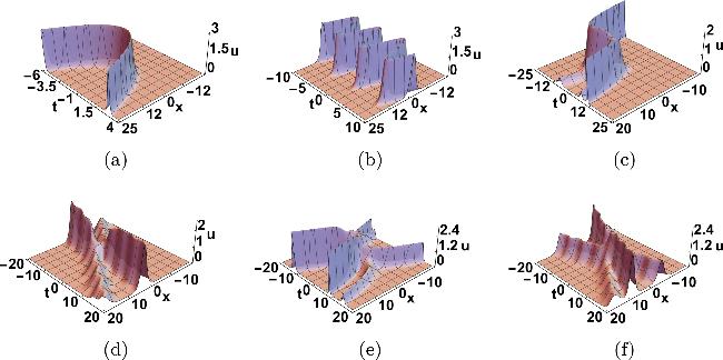
Figure 1. X-shaped soliton: one soliton with k11 = 1, k12 = 2, k13 = 3, c = 2, d = 0.5, g = 0.3, z = 0, t = 0 (a) a(t) = 1, b(t) = 0.5t, α(t) = 0.05t2, β(t) = 1; (b) $a(t)=\sin (t)$, $b(t)=\cos (t)$, $\alpha (t)=\sin (t)$, $\beta (t)=\cos (t)$. Two soliton with k11 = 0.5, k12 = 1, k13 = 1.5, k21 = 1.2, k22 = 1.5, k23 = 0.3, c = 1, d = 0.4, g = 0.2, z = 0, t = 0; (c) a(t) = 0.01t2, b(t) = 0.1t, α(t) = 0.01t2, β(t) = 0.1t; (d) $a(t)=0.3\sin (t)$, $b(t)=0.1\cos (t),\alpha (t)=0.4$, $\beta (t)=0.3\cos (t)$. Three soliton with k11 = − 1, k12 = 0.65, k13 = 1.5, k21 = 1.4, k22 = 1.5, k23 = 1.3, k31 = 0.7, k32 = 1.2, k33 = 0.2, c = 1, d = − 0.4, g = − 0.3, z = 0, t = 0; (e) a(t) = 0.01t2, b(t) = 0.2t, α(t) = 0.01t2, β(t) = 0.2t; (f) $a(t)=0.3\sin (t)$, b(t) = 0.1 cos (t), α(t) = 0.4, $\beta (t)=0.3\cos (t)$. |
3.2. Y-shaped soliton
In order to obtain the Y-shaped N-soliton solution, we make the assumption that 34 ) and (35 ) [37–39]. Inserting equation (34 ) into equation (13 ) leads to
$\begin{eqnarray}\begin{array}{l}\exp ({A}_{ij})=0,\\ (N=L+P,1\leqslant j\lt s\leqslant L,\,L\lt j\lt s\leqslant N),\end{array}\end{eqnarray}$
with $\begin{eqnarray}\begin{array}{r}{\theta }_{i}={k}_{i1}x+{k}_{i2}y+{k}_{i3}z+{f}_{i}(t),\end{array}\end{eqnarray}$
$\begin{eqnarray}\begin{array}{rcl}{f}_{i}(t) & = & \displaystyle \int \left(-{k}_{i1}a(t)-\left(4c{k}_{i1}^{3}+d\frac{{k}_{i2}^{2}}{{k}_{i1}}+g\frac{{k}_{i2}{k}_{i3}}{{k}_{i1}}\right.\right.\\ & & \left.\left.+\frac{{g}^{2}{k}_{i3}^{2}}{4d{k}_{i1}}\right)b(t)-{k}_{i2}\alpha (t)-{k}_{i3}\beta (t)\right)\,{\rm{d}}t,\end{array}\end{eqnarray}$
where i = 1, 2, ⋯ , n based on equations ( $\begin{eqnarray}{k}_{s2}=\frac{2d{k}_{s1}{k}_{j2}+g({k}_{s1}{k}_{j3}-{k}_{j1}{k}_{s3})\pm 2\sqrt{3cd}({k}_{j1}-{k}_{s1}){k}_{j1}{k}_{s1}}{2d{k}_{j1}},\end{eqnarray}$
with cd > 0.When N = 1, the Y-shaped soliton solution is consistent with the X-shaped soliton solution. When it comes to N = 2, L = 2, P = 0, the Y-shaped soliton is called a ‘two-resonance Y-shaped soliton', whose expression is 40 ), equation (41 ) and
$\begin{eqnarray}u=6c{\left(\mathrm{ln}(1+{{\rm{e}}}^{{\theta }_{1}}+{{\rm{e}}}^{{\theta }_{2}})\right)}_{xx},\end{eqnarray}$
with the constriction of equation ( $\begin{eqnarray}{k}_{22}=\frac{2d{k}_{21}{k}_{12}+g({k}_{13}{k}_{21}-{k}_{11}{k}_{23})\pm 2\sqrt{3cd}({k}_{11}-{k}_{21}){k}_{11}{k}_{21}}{2d{k}_{11}}.\end{eqnarray}$
When N = 3, L = 3, P = 0, the three-resonance Y-shaped soliton can be obtained in the form of
$\begin{eqnarray}\begin{array}{r}u=6c{\left(\mathrm{ln}(1+{{\rm{e}}}^{{\theta }_{1}}+{{\rm{e}}}^{{\theta }_{2}}+{{\rm{e}}}^{{\theta }_{3}})\right)}_{xx},\end{array}\end{eqnarray}$
$\begin{eqnarray}\begin{array}{r}{k}_{22}=\frac{2d{k}_{21}{k}_{12}+g({k}_{13}{k}_{21}-{k}_{11}{k}_{23})\pm 2\sqrt{3cd}({k}_{11}-{k}_{21}){k}_{11}{k}_{21}}{2d{k}_{11}},\end{array}\end{eqnarray}$
$\begin{eqnarray}\begin{array}{r}{k}_{32}=\frac{2{d}^{2}{k}_{21}{k}_{31}({k}_{11}-{k}_{31})+gd({k}_{13}{k}_{31}-{k}_{11}{k}_{33})({k}_{11}-{k}_{21})\pm 2\sqrt{3cd}{k}_{11}{k}_{31}({k}_{11}-{k}_{12})({k}_{11}-{k}_{31})}{2{d}^{2}{k}_{11}({k}_{11}-{k}_{21})}.\end{array}\end{eqnarray}$
For P ≠ 0, take N = 4, L = 2, P = 2 as an example. The Y-shaped soliton is the interaction between two-resonance Y-shaped solitons, whose form is 17 ), one can get the expression of ${{\rm{e}}}^{{A}_{ij}}$, k22 and k42 consistent with equations (36 ) and (42 ). Figures 2 and 3 present the visual representations of the Y-shaped soliton solutions corresponding to equation (4 ). In figure 2, it can be seen that a two-resonant Y-shaped soliton has two branches emerging from the main wave, whose amplitude is larger than its branches, while a three-resonant Y-shaped soliton has three. Figure 3 shows the interaction phenomena of resonance Y-shaped solutions as time passes in detail. With the passage of time, the wave crest shifts in its spatial position, yet the wave shape remains largely unchanged.
$\begin{eqnarray}\begin{array}{rcl}\phi & = & 1+{{\rm{e}}}^{{\theta }_{1}}+{{\rm{e}}}^{{\theta }_{2}}+{{\rm{e}}}^{{\theta }_{3}}+{{\rm{e}}}^{{\theta }_{4}}+{{\rm{e}}}^{{\theta }_{1}+{\theta }_{3}+{A}_{13}}\\ & & +{{\rm{e}}}^{{\theta }_{1}+{\theta }_{4}+{A}_{14}}+{{\rm{e}}}^{{\theta }_{2}+{\theta }_{3}+{A}_{23}}+{{\rm{e}}}^{{\theta }_{2}+{\theta }_{4}+{A}_{24}},\end{array}\end{eqnarray}$
$\begin{eqnarray}\begin{array}{r}u=6c{(\mathrm{ln}\phi )}_{xx}.\end{array}\end{eqnarray}$
Let $\begin{eqnarray}\begin{array}{rcl}{F}_{i} & = & 0\,(i=3,4,\cdots \,),\,\varepsilon =1,\\ {F}_{1} & = & 1+{{\rm{e}}}^{{\theta }_{1}}+{{\rm{e}}}^{{\theta }_{2}}+{{\rm{e}}}^{{\theta }_{3}},+{{\rm{e}}}^{{\theta }_{4}},\end{array}\end{eqnarray}$
$\begin{eqnarray}\begin{array}{rcl}{F}_{2} & = & {{\rm{e}}}^{{\theta }_{1}+{\theta }_{3}+{A}_{13}}+{{\rm{e}}}^{{\theta }_{1}+{\theta }_{4}+{A}_{14}}+{{\rm{e}}}^{{\theta }_{2}+{\theta }_{3}+{A}_{23}}\\ & & +{{\rm{e}}}^{{\theta }_{2}+{\theta }_{4}+{A}_{24}},\end{array}\end{eqnarray}$
and insert them into equation (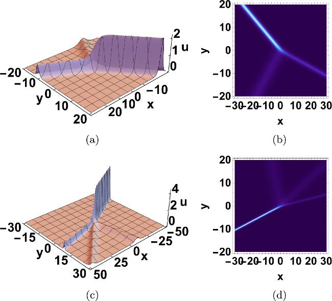
Figure 2. Two-resonance Y-shaped soliton with k11 = 1.2, k12 = 1.5, k13 = 0.3, k21 = 0.5, k23 = 1, c = 1, d = 0.5, g = 0.2, k22 = − 0.407, a(t) = 0.25, b(t) = 0.1, α(t) = 0.3, β(t) = 0.4, z = 0, t = 0; (a) 3D plots: u(x, y, 0, 0); (b) u(x, y, 0, 0). Three-resonance Y-shaped soliton with k11 = − 1, k12 = 0.65, k13 = 1.5, k21 = 0.7, k23 = 0.2, k31 = − 0.5, k33 = 1.3, c = 1, d = 0.4, g = 0.3, k22 = − 4.183, k32 = 0.803, a(t) = 0.01t2, b(t) = 0.2t, α(t) = 0.01t2, β(t) = 0.2t, z = 0, t = 0; (c) 3D plots: u(x, y, 0, 0); (d) u(x, y, 0, 0). |
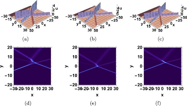
Figure 3. The interaction phenomena of two-resonance Y-shaped soliton with k11 = 1, k12 = 2.5, k13 = 0.6, k21 = − 0.5, k23 = 1.2, k31 = − 0.7, k32 = 0.9, k33 = 0.6, k41 = 1, k43 = 0.5, c = 1, d = 0.5, g = 0.3, k22 = − 2.887, k42 = − 5.857, a(t) = 0.01t2, b(t) = 0.2t, α(t) = 2t, β(t) = − 1, z = 0; (a) 3D plots: u(x, y, 0, − 2); (b) 3D plots: u(x, y, 0, 0); (c) 3D plots: u(x, y, 0, 2); (d) u(x, y, 0, − 2); (e) u(x, y, 0, 0); (f) u(x, y, 0, 2). |
4. Lump, breather and interaction solutions
4.1. Lump solution
Assuming 13 ), we can find that 13 ) turns into
$\begin{eqnarray}\begin{array}{rcl}\phi (x,y,z,t) & = & {({k}_{11}x+{k}_{12}y+{k}_{13}+{f}_{1}(t))}^{2}\\ & & +{({k}_{21}x+{k}_{22}y+{k}_{23}+{f}_{2}(t))}^{2}\\ & & +m,\,m\gt 0\end{array}\end{eqnarray}$
and inserting it into equation ( $\begin{eqnarray}\begin{array}{r}{f}_{1}(t)=\displaystyle \int \frac{{N}_{2}}{4d({k}_{11}^{2}+{k}_{21}^{2})}{\rm{d}}t,\end{array}\end{eqnarray}$
$\begin{eqnarray}\begin{array}{r}{f}_{2}(t)=\displaystyle \int \frac{{N}_{3}}{4d({k}_{11}^{2}+{k}_{21}^{2})}{\rm{d}}t,\end{array}\end{eqnarray}$
where $\begin{eqnarray}\begin{array}{rcl}{N}_{2} & = & -4d({k}_{11}^{2}+{k}_{21}^{2})({k}_{11}a(t)+{k}_{12}\alpha (t)+{k}_{13}\beta (t))\\ & & +{g}^{2}({k}_{11}{k}_{23}^{2}-{k}_{11}{k}_{13}^{2}-2{k}_{13}{k}_{21}{k}_{23})b(t)\\ & & +4{d}^{2}({k}_{11}{k}_{22}^{2}-2{k}_{12}{k}_{21}{k}_{22})b(t)+4dg({k}_{11}{k}_{22}{k}_{23}\\ & & -{k}_{13}{k}_{21}{k}_{22}-{k}_{12}{k}_{21}{k}_{23})b(t),\end{array}\end{eqnarray}$
$\begin{eqnarray}\begin{array}{rcl}{N}_{3} & = & -4d({k}_{11}^{2}+{k}_{21}^{2})({k}_{21}a(t)+{k}_{22}\alpha (t)+{k}_{23}\beta (t))\\ & & +{g}^{2}({k}_{13}{k}_{21}^{2}-{k}_{21}{k}_{23}^{2}-2{k}_{11}{k}_{13}{k}_{23})b(t)\\ & & +4{d}^{2}(-{k}_{12}{k}_{21}^{2}-2{k}_{11}{k}_{12}{k}_{22})b(t)+4dg\\ & & \times (-{k}_{21}{k}_{22}{k}_{23}-{k}_{11}{k}_{13}{k}_{22}+{k}_{12}{k}_{13}{k}_{21})b(t).\end{array}\end{eqnarray}$
Thus, equation ( $\begin{eqnarray}\frac{4\left(12cd{({k}_{11}^{2}+{k}_{21}^{2})}^{3}+{(2d{k}_{12}{k}_{21}+g{k}_{13}{k}_{21}-2d{k}_{11}{k}_{22}-g{k}_{11}{k}_{23})}^{2}m\right)b(t)}{{k}_{11}^{2}+{k}_{21}^{2}}=0.\end{eqnarray}$
Therefore, the lump solutions of equation (4 ) can be obtained as below,53 ) and (54 ).
$\begin{eqnarray}\begin{array}{rcl}\phi (x,y,z,t) & = & {({k}_{11}x+{k}_{12}y+{k}_{13}+{f}_{1}(t))}^{2}\\ & & +{({k}_{21}x+{k}_{22}y+{k}_{23}+{f}_{2}(t))}^{2}+m,\end{array}\end{eqnarray}$
$\begin{eqnarray}\begin{array}{r}m=\frac{-12cd{({k}_{11}^{2}+{k}_{21}^{2})}^{3}}{{(2d{k}_{12}{k}_{21}+g{k}_{13}{k}_{21}-2d{k}_{11}{k}_{22}-g{k}_{11}{k}_{23})}^{2}},\end{array}\end{eqnarray}$
where cd < 0 and f1(t), f2(t) satisfy equations (4.2. Breather solution
The derivation source of the m-breather solution is closely related to the 2m-soliton solution. Taking the two-soliton solution as the foundation, we put forward the assumption that
$\begin{eqnarray}\begin{array}{rcl}\eta & = & ({k}_{11}+{k}_{12}{\rm{i}})x+({k}_{21}+{k}_{22}{\rm{i}})y\\ & & +({k}_{31}+{k}_{32}{\rm{i}})z+{f}_{1}(t),\end{array}\end{eqnarray}$
$\begin{aligned}f_{1}(t)= & \int\left(-\left(k_{11}+k_{12} \mathrm{i}\right) a(t)-\left(4 c\left(k_{11}+k_{12} \mathrm{i}\right)^{3}\right.\right. \\& +d \frac{\left(k_{21}+k_{22} \mathrm{i}\right)^{2}}{\left(k_{11}+k_{12} \mathrm{i}\right)}+g \frac{\left(k_{21}+k_{22} \mathrm{i}\right)\left(k_{31}+k_{32} \mathrm{i}\right)}{\left(k_{11}+k_{12} \mathrm{i}\right)} \\& \left.+\frac{g^{2}\left(k_{31}+k_{32} \mathrm{i}\right)^{2}}{4 d\left(k_{11}+k_{12} \mathrm{i}\right)}\right) b(t)-\left(k_{21}+k_{22} \mathrm{i}\right) \alpha(t) \\& \left.-\left(k_{31}+k_{32} \mathrm{i}\right) \beta(t)\right) \mathrm{d} t .\end{aligned}$
Setting17 ), we can get
$\begin{eqnarray}\begin{array}{r}\begin{array}{l}{R}_{1}={\rm{Re}}(\eta )={k}_{11}x+{k}_{21}y+{k}_{31}z+\displaystyle \int \left(-{k}_{11}a(t)\right.\\ -\,{k}_{21}\alpha (t)-{k}_{31}\beta (t)+c{k}_{11}(-{k}_{11}^{2}+3{k}_{12}^{2})b(t)\\ -\,d\frac{{k}_{11}{k}_{21}^{2}+2{k}_{12}{k}_{21}{k}_{22}-{k}_{11}{k}_{22}^{2}}{{k}_{11}^{2}+{k}_{12}^{2}}b(t)\\ +\,g\frac{-{k}_{11}{k}_{21}{k}_{31}-{k}_{12}{k}_{22}{k}_{31}-{k}_{12}{k}_{21}{k}_{32}+{k}_{11}{k}_{22}{k}_{32}}{{k}_{11}^{2}+{k}_{12}^{2}}b(t)\\ +\,\left.\frac{{g}^{2}}{4d({k}_{11}^{2}+{k}_{12}^{2})}(-{k}_{11}{k}_{31}^{2}-2{k}_{12}{k}_{31}{k}_{32}+{k}_{11}{k}_{32}^{2})\right){\rm{d}}t,\end{array}\end{array}\end{eqnarray}$
$\begin{eqnarray}\begin{array}{r}\begin{array}{l}{I}_{1}={\rm{Im}}(\eta )={k}_{12}x+{k}_{22}y+{k}_{32}z+\displaystyle \int \left(-{k}_{12}a(t)\right.\\ -\,{k}_{22}\alpha (t)-{k}_{32}\beta (t)+c{k}_{12}(-3{k}_{11}^{2}+{k}_{12}^{2})b(t)\\ +\,d\frac{{k}_{12}{k}_{21}^{2}-2{k}_{11}{k}_{21}{k}_{22}-{k}_{12}{k}_{22}^{2}}{{k}_{11}^{2}+{k}_{12}^{2}}b(t)\\ +\,g\frac{{k}_{12}{k}_{21}{k}_{31}-{k}_{11}{k}_{22}{k}_{31}-{k}_{11}{k}_{21}{k}_{32}-{k}_{11}{k}_{31}{k}_{32}}{{k}_{11}^{2}+{k}_{12}^{2}}b(t)\\ \left.+\,\frac{{g}^{2}}{4d({k}_{11}^{2}+{k}_{12}^{2})}({k}_{12}{k}_{31}^{2}-2{k}_{11}{k}_{31}{k}_{32}-{k}_{12}{k}_{32}^{2})\right){\rm{d}}t,\end{array}\end{array}\end{eqnarray}$
$\begin{eqnarray}\begin{array}{r}\phi (x,y,z,t)=1+2\cos ({I}_{1}){{\rm{e}}}^{{R}_{1}}+{a}_{12}{{\rm{e}}}^{2{R}_{1}},\end{array}\end{eqnarray}$
and inserting them into equation ( $\begin{eqnarray}{a}_{12}=\frac{{N}_{4}}{{G}_{4}},\end{eqnarray}$
where $\begin{eqnarray}\begin{array}{rcl}{N}_{4} & = & -12cd{k}_{11}^{4}{k}_{12}^{2}-24cd{k}_{11}^{2}{k}_{12}^{4}-12cd{k}_{12}^{6}\\ & & +4{d}^{2}{k}_{12}^{2}{k}_{21}^{2}-8{d}^{2}{k}_{11}{k}_{12}{k}_{21}{k}_{22}+4{d}^{2}{k}_{11}^{2}{k}_{22}^{2}\\ & & +4dg{k}_{12}^{2}{k}_{21}{k}_{31}-4dg{k}_{11}{k}_{12}{k}_{22}{k}_{31}\\ & & +{g}^{2}{k}_{12}{k}_{31}^{2}-4dg{k}_{11}{k}_{12}{k}_{21}{k}_{32}\\ & & +4dg{k}_{11}^{2}{k}_{22}{k}_{32}-2{g}^{2}{k}_{11}{k}_{12}{k}_{31}{k}_{32}+{g}^{2}{k}_{11}^{2}{k}_{32}^{2},\end{array}\end{eqnarray}$
$\begin{eqnarray}\begin{array}{rcl}{G}_{4} & = & 12cd{k}_{11}^{6}+24cd{k}_{11}^{4}{k}_{12}^{2}+12cd{k}_{11}^{2}{k}_{12}^{4}+4{d}^{2}{k}_{12}^{2}{k}_{21}^{2}\\ & & -8{d}^{2}{k}_{11}{k}_{12}{k}_{21}{k}_{22}+4{d}^{2}{k}_{11}^{2}{k}_{22}^{2}\\ & & +4dg{k}_{12}^{2}{k}_{21}{k}_{31}-4dg{k}_{11}{k}_{12}{k}_{22}{k}_{31}\\ & & +{g}^{2}{k}_{12}{k}_{31}^{2}-4dg{k}_{11}{k}_{12}{k}_{21}{k}_{32}\\ & & +4dg{k}_{11}^{2}{k}_{22}{k}_{32}-2{g}^{2}{k}_{11}{k}_{12}{k}_{31}{k}_{32}+{g}^{2}{k}_{11}^{2}{k}_{32}^{2}.\end{array}\end{eqnarray}$
Therefore, φ(x, y, z, t) and u(x, y, z, t), that is, the breather solutions can be obtained.
The figures of the lump solitons and breather solutions of equation (4 ) are shown in figure 4. It is observable that during the propagation process of the lump waves, neither their shape nor their amplitude undergoes any change as time passes or z alters. As to breather solitons, it is clear that as time progresses or z changes, the breather travels in a parallel manner over the (x, y) − plane, and throughout this process, it maintains its initial geometric structure without noticeable alterations.
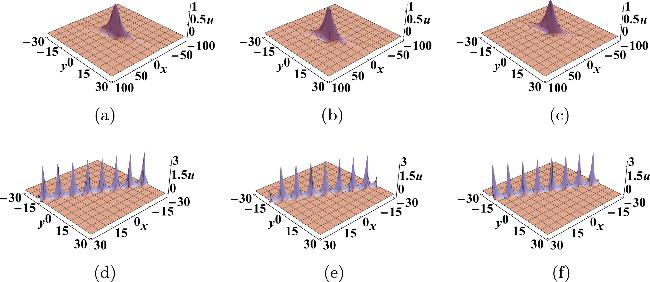
Figure 4. Lump solution with k11 = 1, k12 = 0.5, k13 = 1.5, k21 = 0.8, k22 = 1.8, k23 = 1.6, c = 1, d = − 0.5, g = 0.3, m = 16.153, a(t) = 0.01t2, b(t) = 0.1t, α(t) = 0.01t2, β(t) = 0.1t; (a) 3D plots: u(x, y, 0, 0); (b) 3D plots: u(x, y, 0, 10); (c) 3D plots: u(x, y, 10, 0). Breather solution with k11 = 0.8, k12 = 1.6, k13 = 1.1, k21 = 0.3, k22 = − 1, k23 = 0.3, c = 0.2, d = − 0.3, g = − 0.2, a12 = 1.752, a(t) = 0.01t2, b(t) = 0.1t, α(t) = 0.01t2, β(t) = 0.1t; (d) 3D plots: u(x, y, 0, 0); (e) 3D plots: u(x, y, 0, 5); (f) 3D plots: u(x, y, 5, 0). |
4.3. Interaction solutions
4.3.1. Interaction between lump soliton and one stripe soliton
To derive the one-lump-one-soliton solutions of equation (4 ), we set φ(x, y, z, t) to be composed of two positive quadratic functions and a single exponential function:
$\begin{eqnarray}\phi (x,y,z,t)={\theta }_{1}^{2}+{\theta }_{2}^{2}+{{\rm{e}}}^{{\theta }_{3}}+m,\end{eqnarray}$
where θi = ki1x + ki2y + ki3z + fi(t), (i = 1, 2, 3), m > 0.Inserting equation (68 ) into equation (17 ) and balancing the coefficients, constraints of fi(t), (i = 1, 2, 3) can therefore be obtained.
$\begin{aligned}f_{3}(t)= & \int\left(-k_{31} a(t)-\left(4 c k_{31}^{3}+\mathrm{d} \frac{k_{32}^{2}}{k_{31}}+g \frac{k_{32} k_{33}}{k_{31}}\right.\right. \\& \left.\left.+\frac{g^{2} k_{33}^{2}}{4 \mathrm{~d} k_{31}}\right) b(t)-k_{32} \alpha(t)-k_{33} \beta(t)\right) \mathrm{d} t,\end{aligned}$
$\begin{eqnarray}\begin{array}{r}{f}_{i}(t)=\displaystyle \int \frac{{N}_{5i}}{{k}_{31}^{2}}{\rm{d}}t\,(i=1,2),\end{array}\end{eqnarray}$
where $\begin{eqnarray}\begin{array}{rcl}{N}_{5i} & = & -{k}_{i1}{k}_{31}^{2}a(t)-{k}_{i2}{k}_{31}^{2}\alpha (t)-{k}_{i3}{k}_{31}^{2}\beta (t)\\ & & -\left(3c{k}_{i1}{k}_{31}^{4}-2d{k}_{i2}{k}_{31}{k}_{32}-g{k}_{i3}{k}_{31}{k}_{32}\right.\\ & & +d{k}_{i1}{32}^{2}-g{k}_{i2}{k}_{31}{k}_{33}-\frac{{g}^{2}}{2d}{k}_{i3}{k}_{31}{k}_{32}\\ & & \left.+g{k}_{i1}{k}_{32}{k}_{33}+\frac{{g}^{2}}{4d}{k}_{i1}{k}_{33}^{2}\right)b(t).\end{array}\end{eqnarray}$
It is noted that there are also constraints of k12, k22 and k32. Here we list two cases.
Case I: It can be solved that
$\begin{eqnarray}\begin{array}{r}{k}_{22}=\frac{2d{k}_{21}{k}_{12}+g({k}_{13}{k}_{21}-{k}_{11}{k}_{23})\pm 2\sqrt{-3cd}({k}_{11}-{k}_{21}){k}_{11}{k}_{21}}{2d{k}_{11}},\end{array}\end{eqnarray}$
$\begin{eqnarray}\begin{array}{r}{k}_{32}=\frac{2{k}_{11}(d{k}_{12}{k}_{31}+g{k}_{13}{k}_{31})-g{k}_{33}({k}_{11}^{2}+{k}_{21}^{2})+\frac{2d{k}_{12}{k}_{21}^{2}{k}_{31}+g{k}_{13}{k}_{21}^{2}{k}_{31}}{{k}_{11}}\pm \frac{2\sqrt{-3cd}{k}_{21}{k}_{31}{k}_{31}({k}_{11}^{2}+{k}_{21}^{2})}{{k}_{11}^{2}}}{2d({k}_{11}^{2}+{k}_{21}^{2})},\end{array}\end{eqnarray}$
with cd < 0. Therefore, the constant term turns to $\begin{eqnarray}48cd({k}_{11}^{2}+{k}_{21}^{2})({k}_{11}^{2}+{k}_{21}^{2}-{k}_{31}^{2}m)b(t)=0,\end{eqnarray}$
thus leading to $m=\frac{{k}_{11}^{2}+{k}_{21}^{2}}{{k}_{31}^{2}}$.Case II: It can be solved that
$\begin{eqnarray}\begin{array}{r}{k}_{12}=\frac{-g{k}_{11}^{2}{k}_{13}{k}_{21}^{2}-g{k}_{13}{k}_{21}^{4}+g{k}_{11}^{3}{k}_{21}{k}_{23}+g{k}_{11}{k}_{21}^{3}{k}_{23}\pm 2\sqrt{-3cd}{k}_{21}{k}_{31}{({k}_{11}^{2}+{k}_{21}^{2})}^{2}}{2d{({k}_{11}^{2}+{k}_{11}^{2})}^{2}},\end{array}\end{eqnarray}$
$\begin{eqnarray}\begin{array}{r}{k}_{32}=\frac{g({k}_{11}{k}_{13}{k}_{31}+{k}_{21}{k}_{23}{k}_{31}-{k}_{11}^{2}{k}_{33}-{k}_{21}^{2}{k}_{33})}{2d({k}_{11}^{2}+{k}_{21}^{2})},\end{array}\end{eqnarray}$
where cd < 0. k22 can also be expressed by ki1, ki3, (i = 1, 2, 3), c, d and g. We omit it because of its length. $m=\frac{{k}_{11}^{2}+{k}_{21}^{2}}{{k}_{31}^{2}}$ can also be obtained by eliminating the constant term.Interactions between the lump soliton and one stripe soliton are shown in figures 5 and 6. We find that during the variation of time t, the relative positions of the lump soliton and the stripe soliton remain unchanged and do not separate in both cases. However, the shapes and position of the solitons in two cases are significantly different even with partially identical coefficients.
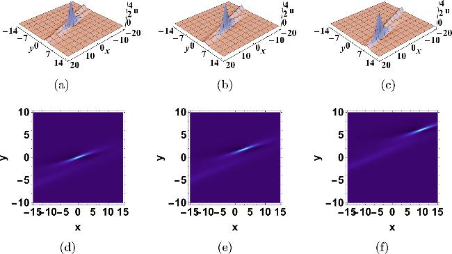
Figure 5. Interaction between lump soliton and one stripe soliton in Case I with k11 = − 1, k12 = 0.65, k13 = 1.5, k21 = 1.4, k23 = 1.3, k31 = 0.7, k33 = 0.2, c = 1, d = − 0.4, g = 0.3, k22 = − 2.562, k32 = 0.443, m = 6.041, a(t) = 0.01t2, b(t) = 0.1t, α(t) = 0.01t2, β(t) = 0.1t; (a) 3D plots: u(x, y, 0, 1); (b) 3D plots: u(x, y, 0, 4); (c) 3D plots: u(x, y, 0, 7); (d) u(x, y, 0, 1); (e) u(x, y, 0, 4); (f) u(x, y, 0, 7). |
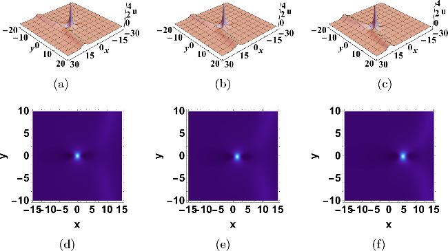
Figure 6. Interaction between lump soliton and one stripe soliton in Case II with k11 = − 1, k13 = 1.5, k21 = 1.4, k23 = 1.3, k31 = 0.7, k33 = 0.2, c = 1, d = − 0.4, g = 0.3, k12 = − 3.287, k22 = − 2.348, k32 = − 0.047, m = 6.041, a(t) = 0.01t2, b(t) = 0.1t, α(t) = 0.01t2, β(t) = 0.1t; (a) 3D plots: u(x, y, 0, 1); (b) 3D plots: u(x, y, 0, 4); (c) 3D plots: u(x, y, 0, 7); (d) u(x, y, 0, 1); (e) u(x, y, 0, 4); (f) u(x, y, 0, 7). |
4.3.2. Interaction between lump soliton and two stripe soliton
Based upon the interaction between the lump soliton and one stripe soliton, we assume an interaction between the lump soliton and two stripe soliton with
$\begin{eqnarray}\phi (x,y,z,t)={\theta }_{1}^{2}+{\theta }_{2}^{2}+{{\rm{e}}}^{{\theta }_{3}}+{{\rm{e}}}^{{\theta }_{4}}+m,\end{eqnarray}$
where θi = ki1x + ki2y + ki3z + fi(t), (i = 1, 2, 3, 4), m > 0.Inserting equation (77 ) into equation (13 ) and balancing the coefficients, constraints of fi(t), (i = 1, 2, 3 ⋯ ) can therefore be obtained.71 ).
$\begin{array}{l}f_{i}(t)=\int\left(-k_{i 1} a(t)-\left(4 c k_{i 1}^{3}+\mathrm{d} \frac{k_{i 2}^{2}}{k_{i 1}}+g \frac{k_{i 2} k_{i 3}}{k_{i 1}}\right.\right. \\\left.\left.+\frac{g^{2} k_{i 3}^{2}}{4 \mathrm{~d} k_{i 1}}\right) b(t)-k_{i 2} \alpha(t)-k_{i 3} \beta(t)\right) \mathrm{d} t, \quad(i=3,4)\end{array}$
$\begin{eqnarray}\begin{array}{r}{f}_{i}(t)=\displaystyle \int \frac{{N}_{5i}}{{k}_{31}^{2}}{\rm{d}}t\,(i=1,2),\end{array}\end{eqnarray}$
where N5i satisfy equation (It can be derived that
$\begin{eqnarray}\begin{array}{r}{k}_{22}=\frac{2d{k}_{21}{k}_{12}+g({k}_{13}{k}_{21}-{k}_{11}{k}_{23})\pm 2\sqrt{-3cd}({k}_{11}-{k}_{21}){k}_{11}{k}_{21}}{2d{k}_{11}},\end{array}\end{eqnarray}$
$\begin{eqnarray}\begin{array}{r}{k}_{32}=\frac{2{k}_{11}(d{k}_{12}{k}_{31}+g{k}_{13}{k}_{31})-g{k}_{33}({k}_{11}^{2}+{k}_{21}^{2})+\frac{2d{k}_{12}{k}_{21}^{2}{k}_{31}+g{k}_{13}{k}_{21}^{2}{k}_{31}}{{k}_{11}}\pm \frac{2\sqrt{-3c{d}^{3}}{k}_{21}{k}_{31}{k}_{11}{k}_{31}({k}_{11}^{2}+{k}_{21}^{2})}{d{k}_{11}^{2}}}{2d({k}_{11}^{2}+{k}_{21}^{2})},\end{array}\end{eqnarray}$
$\begin{eqnarray}\begin{array}{r}{k}_{42}=\frac{2{k}_{11}(d{k}_{12}{k}_{31}+g{k}_{13}{k}_{31})-g{k}_{43}({k}_{11}^{2}+{k}_{21}^{2})+\frac{2d{k}_{12}{k}_{21}^{2}{k}_{31}+g{k}_{13}{k}_{21}^{2}{k}_{31}}{{k}_{11}}\pm \frac{2\sqrt{-3c{d}^{3}}{k}_{21}{k}_{31}{k}_{11}{k}_{31}({k}_{11}^{2}+{k}_{21}^{2})}{d{k}_{11}^{2}}}{2d({k}_{11}^{2}+{k}_{21}^{2})},\end{array}\end{eqnarray}$
$\begin{eqnarray*}\begin{array}{r}{k}_{41}={k}_{31},\,m=\frac{{k}_{11}^{2}+{k}_{21}^{2}}{{k}_{31}^{2}}.\end{array}\end{eqnarray*}$
The profiles of the one-lump-two-soliton are shown in figure 7. Similarly to the one-lump-one-soliton, as time t changes, the relative positions of the lump soliton and the stripe soliton remain constant with no separation occurring between them.
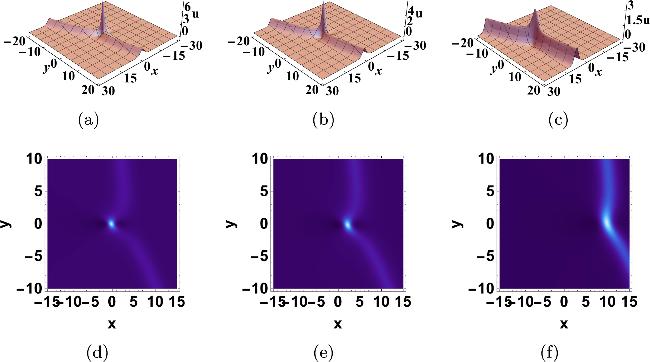
Figure 7. Interaction between lump soliton and two stripe soliton with k11 = 1, k12 = − 1.2, k13 = 0.8, k21 = − 0.6, k23 = 0.7, k31 = 0.7, k33 = 1, k43 = 0.6, c = 1, d = − 0.4, g = 0.3, k22 = − 2.562, k32 = 0.443, k42 = 0.368, m = 1.36, a(t) = 0.01t2, b(t) = 0.1t, α(t) = 0.01t2, β(t) = 0.1t; (a) 3D plots: u(x, y, 0, 1); (b) 3D plots: u(x, y, 0, 4); (c) 3D plots: u(x, y, 0, 8); (d) u(x, y, 0, 1); (e) u(x, y, 0, 4); (f) u(x, y, 0, 8). |
4.3.3. Interaction between breather soliton and one soliton
To discover the one-breather-one-soliton solution, which is a combination of the breather soliton and one soliton for equation (4 ), we hypothesize that 62 ) and (63 ).
$\begin{eqnarray}\begin{array}{rcl}\phi (x,y,t) & = & 1+2\cos ({I}_{1}){{\rm{e}}}^{{R}_{1}}+{{\rm{e}}}^{{\theta }_{3}}+{a}_{12}{{\rm{e}}}^{2{R}_{1}}\\ & & +{a}_{13}{{\rm{e}}}^{{R}_{1}+{I}_{1}{\rm{i}}+{\theta }_{3}}+\overline{{a}_{13}}{{\rm{e}}}^{{R}_{1}-{I}_{1}{\rm{i}}+{\theta }_{3}}+{a}_{123}{{\rm{e}}}^{2{R}_{1}+{\theta }_{3}},\end{array}\end{eqnarray}$
$\begin{eqnarray}\begin{array}{r}{\theta }_{3}={k}_{31}x+{k}_{32}y+{k}_{33}z+{f}_{3}(t),\end{array}\end{eqnarray}$
where R1 and I1 satisfy equations (To fulfill the conditions of breather soliton and one soliton discussed above, it should be satisfied that 66 ) and (67 ).
$\begin{eqnarray}\begin{array}{r}{a}_{12}=\frac{{N}_{4}}{{G}_{4}},\end{array}\end{eqnarray}$
$\begin{array}{l}f_{3}(t)=\int\left(-k_{31} a(t)-\left(4 c k_{31}^{3}+\mathrm{d} \frac{k_{32}^{2}}{k_{31}}+g \frac{k_{32} k_{33}}{k_{31}}\right.\right. \\\left.\left.+\frac{g^{2} k_{33}^{2}}{4 \mathrm{~d} k_{31}}\right) b(t)-k_{32} \alpha(t)-k_{33} \beta(t)\right) \mathrm{d} t,\end{array}$
where N4 and G4 satisfy equations (By substituting equation (83 ) into equation (17 ), we can also derive expressions for a13 and a123. Given the considerable length of this derivation process, we opt to omit it here.
Profiles of the one-breather-one-soliton can also be described by choosing appropriate parameters in figure 8. It can be seen that throughout the temporal evolution, the breather soliton and one soliton propagate in a phase-locked manner, with each preserving its original, coherent waveform.
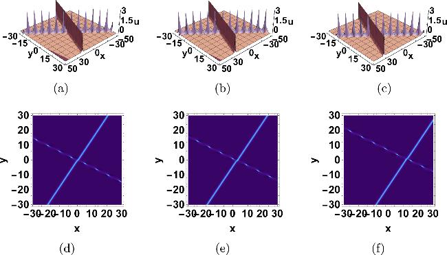


Figure 8. Interaction between breather soliton and one soliton with k11 = 0.8, k12 = 0.3, k13 = 3, k21 = − 1.6, k22 = − 1, k23 = − 2, k31 = 1.1, k32 = 0.2, k33 = 1.2, c = 0.2, d = − 0.3, g = − 0.2, a12 = 1.752, a13 = 0.470 + 1.367i, a123 = 3.664, a(t) = 0.01t2, b(t) = 0.1t, α(t) = 0.01t2, β(t) = 0.1t (a) 3D plots: u(x, y, 0, 1); (b) 3D plots: u(x, y, 0, 5); (c) 3D plots: u(x, y, 0, 10); (d) u(x, y, 0, 1); (e) u(x, y, 0, 5); (f) u(x, y, 0, 10). |
5. Various other solutions
5.1. tanh soliton solution
Inserting equation (87 ) into equation (4 ) and taking the compatibility conditions equation (8 ) into account, we can obtain that 89 ) and (90 ).
$\begin{eqnarray}\begin{array}{r}{a}_{1}=-6c{k}_{1}^{2},\end{array}\end{eqnarray}$
$\begin{eqnarray}\begin{array}{r}{f}_{0}(t)=\displaystyle \int \frac{{N}_{6}}{4d{k}_{1}}\,{\rm{d}}t,\end{array}\end{eqnarray}$
where $\begin{eqnarray}\begin{array}{rcl}{N}_{6} & = & -4d{k}_{1}^{2}a(t)-40{a}_{1}d{k}_{1}^{2}b(t)-4{d}^{2}{k}_{2}^{2}b(t)\\ & & -4dg{k}_{2}{k}_{3}b(t)-{g}^{2}{k}_{3}^{2}b(t)-208cd{k}_{1}^{4}b(t)\\ & & -4d{k}_{1}{k}_{2}\alpha (t)-4d{k}_{1}{k}_{3}\beta (t)-8d{k}_{1}^{2}b(t){f}_{1}(t),\end{array}\end{eqnarray}$
and f1(t) is an arbitrary function. Therefore, the following soliton solution is acquired: $\begin{eqnarray}\begin{array}{rcl}u(x,y,z,t) & = & {f}_{1}(t)-6c{k}_{1}^{2}{\tanh }^{2}({k}_{1}x+{k}_{2}y\\ & & +{k}_{3}z+{f}_{0}(t)),\end{array}\end{eqnarray}$
where f0(t) satisfies equations (5.2. Periodic solution
Following the tan scheme, the periodic solution is considered:
$\begin{eqnarray}\begin{array}{rcl}u(x,y,z,t) & = & {f}_{1}(t)+{a}_{1}{\tan }^{2}({k}_{1}x+{k}_{2}y\\ & & +{k}_{3}z+{f}_{0}(t)),\end{array}\end{eqnarray}$
where f0(t) also represents the dispersion relation [15].Substituting equation (92 ) into equation (4 ) can obtain 94 ) and (95 ).
$\begin{eqnarray}\begin{array}{r}{a}_{1}=-6c{k}_{1}^{2},\end{array}\end{eqnarray}$
$\begin{eqnarray}\begin{array}{r}{f}_{0}(t)=\displaystyle \int \frac{{N}_{7}}{4d{k}_{1}}\,{\rm{d}}t,\end{array}\end{eqnarray}$
where $\begin{eqnarray}\begin{array}{rcl}{N}_{7} & = & -4d{k}_{1}^{2}a(t)-40{a}_{1}d{k}_{1}^{2}b(t)-4{d}^{2}{k}_{2}^{2}b(t)\\ & & -4dg{k}_{2}{k}_{3}b(t)-{g}^{2}{k}_{3}^{2}b(t)-272cd{k}_{1}^{4}b(t)\\ & & -4d{k}_{1}{k}_{2}\alpha (t)-4d{k}_{1}{k}_{3}\beta (t)-8d{k}_{1}^{2}b(t){f}_{1}(t),\end{array}\end{eqnarray}$
and f1(t) is an arbitrary function. Therefore, the following periodic solution is derived: $\begin{eqnarray}\begin{array}{rcl}u(x,y,z,t) & = & {f}_{1}(t)-6c{k}_{1}^{2}{\tan }^{2}({k}_{1}x+{k}_{2}y\\ & & +{k}_{3}z+{f}_{0}(t)),\end{array}\end{eqnarray}$
where f0(t) satisfies equations (5.3. Ratio of trigonometric function
Case I:
In this case, we assume
$\begin{eqnarray}u(x,y,z,t)=\frac{{a}_{0}}{1+{a}_{1}\cos ({k}_{1}x+{k}_{2}y+{k}_{3}z+{f}_{0}(t))}.\end{eqnarray}$
Substituting equation (97 ) into equation (4 ) can get
$\begin{eqnarray}\begin{array}{r}{a}_{0}=-6c{k}_{1}^{2},\end{array}\end{eqnarray}$
$\begin{eqnarray}\begin{array}{r}{f}_{0}(t)=\displaystyle \int \frac{{N}_{8}}{4d{k}_{1}}\,{\rm{d}}t,\end{array}\end{eqnarray}$
$\begin{eqnarray}\begin{array}{r}{a}_{1}=\pm 1,\end{array}\end{eqnarray}$
where $\begin{eqnarray}\begin{array}{rcl}{N}_{8} & = & -4d{k}_{1}^{2}a(t)-40{a}_{1}d{k}_{1}^{2}b(t)-4{d}^{2}{k}_{2}^{2}b(t)\\ & & -4dg{k}_{2}{k}_{3}b(t)-{g}^{2}{k}_{3}^{2}b(t)-116cd{k}_{1}^{4}b(t)\\ & & -4d{k}_{1}{k}_{2}\alpha (t)-4d{k}_{1}{k}_{3}\beta (t)-8d{k}_{1}^{2}b(t){f}_{1}(t).\end{array}\end{eqnarray}$
Case II:
In this case, we consider
$\begin{eqnarray}u(x,y,z,t)=\frac{{a}_{0}}{1+{a}_{1}\sec ({k}_{1}x+{k}_{2}y+{k}_{3}z+{f}_{0}(t))}.\end{eqnarray}$
Inserting equation (102 ) into equation (4 ) can obtain
$\begin{eqnarray}\begin{array}{r}{a}_{0}=6c{k}_{1}^{2},\\ \end{array}\end{eqnarray}$
$\begin{eqnarray}\begin{array}{r}{f}_{0}(t)=\displaystyle \int \frac{{N}_{9}}{4d{k}_{1}}\,{\rm{d}}t,\\ \end{array}\end{eqnarray}$
$\begin{eqnarray}\begin{array}{r}{a}_{1}=\pm 1,\end{array}\end{eqnarray}$
where $\begin{eqnarray}\begin{array}{rcl}{N}_{9} & = & -4d{k}_{1}^{2}a(t)-40{a}_{1}d{k}_{1}^{2}b(t)-4{d}^{2}{k}_{2}^{2}b(t)\\ & & -4dg{k}_{2}{k}_{3}b(t)-{g}^{2}{k}_{3}^{2}b(t)+100cd{k}_{1}^{4}b(t)\\ & & -4d{k}_{1}{k}_{2}\alpha (t)-4d{k}_{1}{k}_{3}\beta (t)-8d{k}_{1}^{2}b(t){f}_{1}(t).\end{array}\end{eqnarray}$
Therefore, the ratio of trigonometric functions in two cases are both obtained.
6. Conclusion
In this paper, a generalized (3+1)-dimension variable-coefficient nonlinear evolution equation equation (4 ) exploring the nonlinear behaviors of waves in ion-acoustic waves in fluid mechanics and plasma physics has been investigated with symbolic computation. The Painlevé integrability has been tested by means of the WTC method and it has been demonstrated that the Painlevé property holds for equation (4 ) under specific constraints on its coefficients. The Hirota bilinear method has been applied to present the bilinear form corresponding to equation (4 ). On the basis of the obtained bilinear forms, we have put forward analytical solutions, covering X-shaped and Y-shaped soliton, lump, breather, and interaction solutions. In addition, an in-depth investigation has been conducted into the propagation characteristics and dynamic behaviors exhibited by these solutions. In addition, we have discussed various other solutions, including $\tanh $ solution, periodic solution, and ratio of trigonometric functions.
It is anticipated that the results obtained herein will provide valuable insights for the further exploration of the generalized (3+1)-dimension variable-coefficient nonlinear evolution equation. Additionally, investigations into more types of interaction solutions, as well as Lie symmetries, Lax pairs, and auto-Bäcklund transformations are also expected to be carried out.