


1. Introduction
Complex nonlinear partial differential equations (PDEs) represent a formidable family of mathematical models that arise in various scientific disciplines, including physics, engineering, and biology. These equations capture intricate interactions and nonlinear behaviors in dynamic systems, making their analysis challenging yet essential. Investigating exact solutions for complex nonlinear PDEs holds significant importance as it provides an elaboration of the considered physical phenomena. Exact solutions serve as benchmarks for numerical methods, validating their accuracy and reliability. Additionally, these solutions provide important insights into the qualitative behavior of the systems represented by the equations, shedding light on the emergence of patterns, solitons, and other complex structures. The discovery of analytical solutions also contributes to the development of analytical tools and methodologies, fostering advancements in the broader understanding of nonlinear dynamics and facilitating the design of innovative solutions to practical problems in diverse scientific and engineering applications.
In [1], the dynamical behavior and optical soliton solutions of the coupled Kaup–Newell equation in birefringent fibers are investigated. Using traveling wave transforms and the homogeneous balance principle, the system is reduced to an ODE. The complete discriminant system method is then employed to derive various soliton solutions, including solitary wave, rational, Jacobian elliptic, and hyperbolic function solutions. In [2], Tang examines the dynamical behavior and dispersive optical solitons of the coupled Schrödinger–Hirota equation in birefringent fibers. Using traveling wave transformations, the system is reduced to a planar dynamical system, from which bell-shaped, periodic, and kink-shaped wave solutions are derived. The complete discriminant system method is then applied to classify all single traveling wave solutions. In [3], a bifurcation analysis of a concatenation model from nonlinear fiber optics is presented. The fixed points of the dynamical system are identified and classified, the system's Hamiltonian is derived, and its phase portraits are examined. By integrating along periodic orbits, the authors successfully retrieve soliton solutions for the model.
In this study, we investigate the complex Ginzburg–Landau equation (CGLE) presented in the following form: 1 ) correspond to linear dispersion, nonlinear frequency shift, and linear gain or loss, respectively, while the right-hand side terms account for more intricate perturbation effects arising from higher-order corrections in the amplitude expansion [13]. The specific form of equation (1 ) considered in this paper incorporates generalized nonlinearity $F\left(| \phi {| }^{2}\right)$ and additional dissipative terms that extend the standard CGLE. Such generalized models arise naturally when deriving amplitude equations from physical systems with more complex nonlinear couplings or when higher-order corrections to the bifurcation scenario become significant [10, 13]. These extensions allow the model to capture phenomena beyond the reach of the standard CGLE, including more diverse soliton dynamics and richer pattern formation scenarios relevant to modern applications in photonics and fluid dynamics.
$\begin{eqnarray}\begin{array}{c}{\rm{i}}{\phi }_{t}+a{\phi }_{{xx}}+F\left(|\phi {|}^{2}\right)\phi \\ =\,\frac{1}{|\phi {|}^{2}{\phi }^{\ast }}\left[\alpha |\phi {|}^{2}{\left(|\phi {|}^{2}\right)}_{{xx}}\right.\\ \left.-\,\beta {\left\{{\left(|\phi {|}^{2}\right)}_{x}\right\}}^{2}\right]+\gamma \phi .\end{array}\end{eqnarray}$
Here, φ(x, t) denotes a function with complex values, and x and t represent spatial and temporal coordinates, respectively. The parameter a accounts for group velocity dispersion and is termed the group-velocity dispersion parameter, as referenced in [4, 5]. The function $F\left(| \phi {| }^{2}\right)$ is a nonlinear potential characterized by ∣φ∣2, with its specific form considered in this study being an anti-cubic expression, given as $F\left(| \phi {| }^{2}\right)=\frac{b}{| \phi {| }^{4}}$ as outlined in [6, 7]. The parameters α and β are empirical constants, as discussed in [6,7], while the parameter γ is associated with detuning effects [8]. Beyond superconductivity, the CGLE has acquired a much broader significance as a canonical amplitude equation in the theory of pattern formation and nonlinear dynamics [9]. Near the onset of a supercritical Hopf bifurcation in oscillatory media, the CGLE arises universally as the equation governing the slow spatiotemporal modulation of the oscillation amplitude [9, 10]. More specifically, when a reaction-diffusion system undergoes a Hopf bifurcation, a multiple-scale analysis yields the CGLE as the reduced amplitude equation for the complex oscillation envelope, provided the system is close to the bifurcation threshold [10]. This derivation establishes the CGLE as a normal form for a wide class of oscillatory media, including chemical oscillations (such as the Belousov–Zhabotinsky reaction), hydrodynamic instabilities, and biological pattern formation [9, 11]. In fluid dynamics, the CGLE describes the evolution of perturbations near the onset of oscillatory instabilities, such as those leading to chaotic dynamics in fluid mechanical systems [11]. It has been extensively studied as a model for turbulent dynamics in nonlinear partial differential equations, serving as a dissipative extension of the nonlinear Schrödinger equation. In nonlinear optics, the CGLE plays a particularly prominent role. It models the propagation of optical pulses in fiber lasers and communication systems, where the balance between gain, loss, dispersion, and nonlinearity gives rise to dissipative solitons [12, 13]. The cubic-quintic version of the CGLE, in particular, has proven essential for describing localized structures in various optical systems with gain and loss. The terms involving α, β and γ in equation (The CGLE is a mathematical model that describes the dynamics of complex scalar fields, particularly in the context of nonlinear wave phenomena. Originally developed in the field of condensed matter physics to explain the behavior of superconductors and superfluids, the CGLE has since found widespread applicability across diverse scientific disciplines. In the realm of nonlinear optics, it serves as a crucial tool for understanding the dynamics of optical pulses and patterns in various media. Additionally, the CGLE has proven instrumental in describing pattern formation in chemical reactions, fluid dynamics, and even biological systems. Its real-world applications extend to the study of spatiotemporal phenomena, such as the formation of coherent structures and the emergence of turbulence, thereby providing valuable insights into complex systems across multiple scientific domains [14–16].
In this study, we demonstrate that solitary waves can be derived under the condition $F\left(| \phi {| }^{2}\right)=b| \phi {| }^{-4}$, for equation (1 ). Through the application of a modified version of the simplest equation method, we derive soliton solutions for equation (1 ), revealing that the amplitude of the soliton solution remains independent of its velocity.
Let us look for the solution of equation (1 ), in the following form:
$\begin{eqnarray}\phi (x,t)={ \mathcal Q }(\xi ){{\rm{e}}}^{{\rm{i}}(\varpi (\xi )-\omega t)},\quad \xi =x-\varrho t,\end{eqnarray}$
where ϱ is a parameter of the solution, and ${ \mathcal Q }(\xi )$ and ϖ(ξ) are new functions that can be determined as follows [21]: $\begin{eqnarray}\begin{array}{l}a(a-2\alpha ){ \mathcal Q }{{ \mathcal Q }}_{\xi \xi }+2a(2\beta -\alpha ){{ \mathcal Q }}_{\xi }^{2}\\ +\,\left[\frac{{\varrho }^{2}}{4}+a(\omega -\gamma )\right]{{ \mathcal Q }}^{2}=0,\end{array}\end{eqnarray}$
and $\begin{eqnarray}\varpi (\xi )=\frac{\varrho \xi }{2a}+\frac{{{ \mathcal K }}_{1}}{ak{A}^{2}}{\int }_{0}^{\xi -{\xi }_{0}}{\left({{\rm{e}}}^{\xi }+{{\rm{e}}}^{-\xi }\right)}^{m}{\rm{d}}\xi +{{ \mathcal K }}_{2},\end{eqnarray}$
where ${{ \mathcal K }}_{2}$ is an arbitrary constant and $m=\frac{4\alpha -2a}{a+4\beta -4\alpha }$.The primary research meaning of this work is to address a fundamental limitation in the analytical treatment of complex nonlinear systems. While nonlinear PDEs like the CGLE are cornerstones of modern physics—describing phenomena from fluid dynamics and nonlinear waves to Bose–Einstein condensation—their analytical solutions are notoriously difficult to obtain. Traditional methods, such as those relying on first-degree or constant-coefficient auxiliary equations, often fail to capture the full dynamical richness of these systems, particularly when parameters vary or when higher-order nonlinearities are present. This creates a critical gap between the mathematical models and our ability to explore their physical implications analytically. The motivation for this paper stems from the need to bridge this gap. The CGLE, in particular, serves as a universal model for systems near a Hopf bifurcation, making its solutions highly sought after for understanding pattern formation, turbulence, and wave propagation. Our work is motivated by the premise that to uncover new and more general wave behaviors, we must move beyond the methodological status quo of constant-coefficient ODEs. We hypothesize that introducing variable coefficients directly into the solving mechanism will yield a richer set of solutions that are more representative of real-world physical systems, which are often non-uniform and subject to varying conditions.Our primary contribution is the development of a new analytical technique that utilizes a VCSDGAE as its sub-equation. This represents a significant methodological departure from existing techniques (e.g., the (G'/G)-method, sine-cosine method) that are constrained by constant coefficients. This innovation provides a more flexible and powerful mathematical ansatz for constructing solutions to nonlinear PDEs.Beyond merely presenting new mathematical expressions, we establish the physical relevance of our results. By performing a linear stability analysis, we rigorously demonstrate the robustness of the obtained soliton solutions against small perturbations. This is a crucial step that confirms the solutions are not just mathematical artifacts but represent potentially observable and stable physical phenomena.
2. Description of method
The utilized technique in the current study, firstly introduced by Hashemi in [22], and then developed to the two-mode Cahn–Allen equation in [23]. This technique utilized in [24] for the third-order Gilson–Pickering equation. In [25], the authors applied this method for the perturbed nonlinear Schrödinger equations. In this manuscript, we investigate a nth-order differential equation characterized by the following form:
$\begin{eqnarray*}{\rm{\Xi }}\left(\xi ,{ \mathcal W },{ \mathcal W }^{\prime} ,\ldots ,{{ \mathcal W }}^{(n)}\right)=0,\end{eqnarray*}$
where ${\rm{\Xi }}\left(\xi ,{ \mathcal W },{ \mathcal W }^{\prime} ,\ldots ,{{ \mathcal W }}^{(n)}\right)$ is a polynomial in the variables ${ \mathcal W },{ \mathcal W }^{\prime} ,\ldots ,{{ \mathcal W }}^{(n)}$.In the current investigation, we propose an approach wherein solutions to the following second-degree Abel's equation also serve as solutions to the equation represented by (3 ):
$\begin{eqnarray}{ \mathcal W }^{\prime} ={\vartheta }_{2}(\xi ){{ \mathcal W }}^{2}+{\vartheta }_{1}(\xi ){ \mathcal W }+{\vartheta }_{0}(\xi ),\end{eqnarray}$
where ϑi(ξ), 0≤i≤2, are arbitrary, smooth functions.Obviously, equation (5 ) is a general form of constant sub-equation methods, such as the tanh method [26, 27], modified extended tanh function method [28, 29], extended hyperbolic function method [30], and the modified extended direct algebraic technique [31–34]. It is important to highlight that in the majority of analytical techniques employing the sub-equation for obtaining exact solutions, the sub-equation is formulated as an ODE with coefficients that remain constant.
To begin with, we present a method for obtaining the equations (5 ) from the specified equation (3 ). One time differentiation of equation (5 ) with respect to ξ, we get 5 ) into (6 ), we obtain 5 ) will also be a solution to (3 ).
$\begin{eqnarray}{{ \mathcal W }}^{{\prime\prime} }(\xi )={\vartheta }_{2}^{\prime} {{ \mathcal W }}^{2}+{\vartheta }_{1}^{\prime} { \mathcal W }+{\vartheta }_{0}^{\prime} +{ \mathcal W }^{\prime} \left[2{\vartheta }_{2}{ \mathcal W }+{\vartheta }_{1}\right].\end{eqnarray}$
Therefore, by substituting ${{ \mathcal W }}^{{\prime} }$ from ( $\begin{eqnarray}\begin{array}{l}{{ \mathcal W }}^{{\prime\prime} }(\xi )={\vartheta }_{2}^{\prime} {{ \mathcal W }}^{2}+{\vartheta }_{1}^{\prime} { \mathcal W }+{\vartheta }_{0}^{\prime} \\ \,+\,\left({\vartheta }_{2}{{ \mathcal W }}^{2}+{\vartheta }_{1}{ \mathcal W }+{\vartheta }_{0}\right)\left[2{\vartheta }_{2}{ \mathcal W }+{\vartheta }_{1}\right]\\ \,=\,2{\vartheta }_{2}^{2}{{ \mathcal W }}^{3}+\left({\vartheta }_{2}^{\prime} +3{\vartheta }_{1}{\vartheta }_{2}\right){{ \mathcal W }}^{2}\\ \,+\,\left({\vartheta }_{1}^{\prime} +{\vartheta }_{1}^{2}+2{\vartheta }_{0}{\vartheta }_{2}\right){ \mathcal W }+\left({\vartheta }_{0}^{\prime} +{\vartheta }_{0}{\vartheta }_{1}\right).\end{array}\end{eqnarray}$
The fundamental concept of this novel approach is explained as follows. By substituting polynomial forms for ${ \mathcal W }^{\prime} ,{{ \mathcal W }}^{{\prime\prime} },\ldots ,{{ \mathcal W }}^{(n)}$ into ${\rm{\Xi }}\left(\xi ,{ \mathcal W },{ \mathcal W }^{\prime} ,\ldots ,{{ \mathcal W }}^{(n)}\right)$, one can obtain a polynomial expressed in terms of ${ \mathcal W }$. By setting the coefficients of this polynomial to zero, an overdetermined system of algebraic and ODEs for ϑi(ξ), 0≤i≤2, is generated. If a solution in the form of ϑ0(ξ), ϑ1(ξ), ϑ2(ξ) exists for this system, then any solution to (The main novelties of this manuscript lie in the development of the “VCSDGAE,” which innovates by utilizing variable-coefficient ODEs within a sub-equation framework, marking a departure from traditional constant-coefficient approaches. The significance of this research is twofold: first, it successfully demonstrates the method's powerful versatility by deriving new analytical solutions for the CGLE, and second, it rigorously validates the physical viability of these solutions through linear stability analysis. By moving beyond constant-coefficient constraints, this work provides a more flexible and effective analytical tool for tackling complex nonlinear phenomena in fields like fluid dynamics and wave propagation, thereby advancing the suite of methodologies available for mathematical physics.
It is also important to acknowledge the potential drawbacks of the proposed method. First, the substitution of the generalized Abel equation into the reduced ODE can, in some cases, lead to an inconsistent system, where no solution exists that satisfies both the original equation and the auxiliary equation simultaneously. This is a critical point where the method fails to yield a valid result for the specific parameter regime under consideration. Second, even when a consistent reduction is achieved, the resulting differential-algebraic system may not be solvable analytically. In such instances, while the method successfully reduces the problem's complexity, obtaining a closed-form solution would require further analytical manipulation or the application of numerical techniques.
3. Main results
In this section, we apply the proposed method to the nonlinear ODE (3 ). For this study, we consider the generalized Abel equation (5 ). Substituting (5 ) into equation (3 ) results in a fifth-degree polynomial in ${ \mathcal W }$, expressed as:
$\begin{eqnarray*}\displaystyle \sum _{i=0}^{4}{S}_{i}{{ \mathcal W }}^{i}=0,\end{eqnarray*}$
where $\begin{eqnarray*}{S}_{0}=16a\left(\beta -\frac{\alpha }{2}\right){\vartheta }_{0}^{2}\left(\xi \right),\end{eqnarray*}$
$\begin{eqnarray*}{S}_{1}=4a\left(a-2\alpha \right){\vartheta }_{0}^{{\prime} }\left(\xi \right)+4a{\vartheta }_{0}\left(\xi \right)\left(a+8\beta -6\alpha \right){\vartheta }_{1}\left(\xi \right),\end{eqnarray*}$
$\begin{eqnarray*}{S}_{2}=4a\left(a-2\alpha \right){\vartheta }_{1}^{{\prime} }\left(\xi \right)+4a\left(a+4\beta -4\alpha \right){\vartheta }_{1}^{2}\left(\xi \right)+8a{\vartheta }_{0}\left(\xi \right)\left(a+4\beta -4\alpha \right){\vartheta }_{2}\left(\xi \right)+{\varrho }^{2}+4a\left(w-\gamma \right),\end{eqnarray*}$
$\begin{eqnarray*}{S}_{3}=4a\left(a-2\alpha \right){\vartheta }_{2}^{{\prime} }\left(\xi \right)+12a\left(a+\frac{8\beta }{3}-\frac{10\alpha }{3}\right){\vartheta }_{2}\left(\xi \right){\vartheta }_{1}\left(\xi \right),\end{eqnarray*}$
$\begin{eqnarray*}{S}_{4}=8a\left(a+2\beta -3\alpha \right){\vartheta }_{2}^{2}\left(\xi \right).\end{eqnarray*}$
Setting Si = 0, i = 0, …, 4, results in a system of differential-algebraic equations (DAEs) with the following sets of solutions:
Family 1: 5 ) transforms into 8 ) concludes: 3 ) and (9 ), the initial exact solution can be expressed as a periodic wave solution in the following form: 4 ). In the general case, for arbitrary values of m, the function ϖ(ξ) takes the form of an integral that cannot be expressed explicitly. Therefore, by setting ξ0 = 0 and considering the following special cases for m, we derive several explicit solutions:
$\begin{eqnarray*}\begin{array}{rcl}{\vartheta }_{1}(\xi ) & = & -\frac{\tan \,\left(\frac{\sqrt{\left(-4a\gamma +4aw+{\varrho }^{2}\right)a\left(a+4\beta -4\alpha \right)}\left({R}_{1}+\xi \right)}{2a\left(a-2\alpha \right)}\right)\sqrt{\left(-4a\gamma +4aw+{\varrho }^{2}\right)a\left(a+4\beta -4\alpha \right)}}{2a\left(a+4\beta -4\alpha \right)},\\ {\vartheta }_{0}(\xi ) & = & {\vartheta }_{2}(\xi )=0,\,{R}_{1}\in {\mathbb{R}}.\end{array}\end{eqnarray*}$
In this scenario, the ODE ( $\begin{eqnarray}{{ \mathcal W }}^{{\prime} }\left(\xi \right)=-\frac{\tan \,\left(\frac{\sqrt{\left(-4a\gamma +4aw+{\varrho }^{2}\right)a\left(a+4\beta -4\alpha \right)}\left({R}_{1}+\xi \right)}{2a\left(a-2\alpha \right)}\right)\sqrt{\left(-4a\gamma +4aw+{\varrho }^{2}\right)a\left(a+4\beta -4\alpha \right)}}{2a\left(a+4\beta -4\alpha \right)}{ \mathcal W }\left(\xi \right).\end{eqnarray}$
Solving the equation ( $\begin{eqnarray}\begin{array}{l}{ \mathcal W }(\xi )={R}_{2}{\left(1+{\tan }^{2}\left(\frac{\sqrt{\left(-4a\gamma +4aw+{\varrho }^{2}\right)a\left(a+4\beta -4\alpha \right)}\left({R}_{1}+\xi \right)}{2a\left(a-2\alpha \right)}\right)\right)}^{-\frac{a-2\alpha }{2a+8\beta -8\alpha }},\\ {R}_{2}\in {\mathbb{R}}.\end{array}\end{eqnarray}$
Therefore, according to ( $\begin{eqnarray}\begin{array}{r}\begin{array}{l}\phi (x,t)={R}_{2}{\left(1+{\tan }^{2}\left(\frac{\sqrt{\left(-4a\gamma +4aw+{\varrho }^{2}\right)a\left(a+4\beta -4\alpha \right)}\left({R}_{1}+x-\varrho t\right)}{2a\left(a-2\alpha \right)}\right)\right)}^{-\frac{a-2\alpha }{2a+8\beta -8\alpha }}\\ \,\times \,{{\rm{e}}}^{{\rm{i}}(\varpi (x-\varrho t)-\omega t)},\end{array}\end{array}\end{eqnarray}$
where ϖ(ξ) is defined by equation (Case 1-1: m = 1.
In this case, we obtain $\alpha =\frac{3a}{8}+\frac{\beta }{2}$, and
$\begin{eqnarray}\varpi (\xi )=\frac{\varrho k{A}^{2}\xi +2{{ \mathcal K }}_{1}{{\rm{e}}}^{\xi }-2{{ \mathcal K }}_{1}{{\rm{e}}}^{-\xi }}{2ak{A}^{2}}.\end{eqnarray}$
Therefore, from equations (10 ) and (11 ) we obtain
$\begin{eqnarray}\begin{array}{r}\begin{array}{l}\phi (x,t)={R}_{2}{\left(1+{\tan }^{2}\left(\frac{\sqrt{\left(-4a\gamma +4aw+{\varrho }^{2}\right)a\left(-\frac{a}{2}+2\beta \right)}\left(-\varrho t+x+{R}_{1}\right)}{2a\left(\frac{a}{4}-\beta \right)}\right)\right)}^{-\frac{\frac{a}{4}-\beta }{-a+4\beta }}\\ \,\times \,{{\rm{e}}}^{{\rm{i}}\left(\frac{\varrho \left(-\varrho t+x\right)}{2a}+\frac{{{ \mathcal K }}_{1}\left({{\rm{e}}}^{-\varrho t+x}-{{\rm{e}}}^{\varrho t-x}\right)}{ak{A}^{2}}-wt\right)}.\end{array}\end{array}\end{eqnarray}$
Case 1-2: m = 2.
In this case, we obtain $\alpha =\frac{a+2\beta }{3}$, and
$\begin{eqnarray}\varpi (\xi )=\frac{-{{ \mathcal K }}_{1}{{\rm{e}}}^{-2\xi }+{{ \mathcal K }}_{1}{{\rm{e}}}^{2\xi }+\xi \left({A}^{2}\varrho k+4{{ \mathcal K }}_{1}\right)}{2ak{A}^{2}}.\end{eqnarray}$
Therefore, from equations (10 ) and (13 ) we obtain
$\begin{eqnarray}\begin{array}{rcl}\phi (x,t) & = & {R}_{2}{\left(1+{\tan }^{2}\left(\frac{\sqrt{\left(-4a\gamma +4aw+{\varrho }^{2}\right)a\left(-\frac{a}{3}+\frac{4\beta }{3}\right)}\left(-\varrho t+x+{R}_{1}\right)}{2a\left(\frac{a}{3}-\frac{4\beta }{3}\right)}\right)\right)}^{-\frac{\frac{a}{3}-\frac{4\beta }{3}}{-\frac{2a}{3}+\frac{8\beta }{3}}}\\ & & \times {{\rm{e}}}^{{\rm{i}}\left(\frac{\varrho \left(-\varrho t+x\right)}{2a}+\frac{{{ \mathcal K }}_{1}\left({{\rm{e}}}^{-4\varrho t+4x}+4\left(-\varrho t+x\right){{\rm{e}}}^{-2\varrho t+2x}-1\right){{\rm{e}}}^{2\varrho t-2x}}{2ak{A}^{2}}-wt\right)}.\end{array}\end{eqnarray}$
Case 1-3: m = 3.
In this case, we obtain $\alpha =\frac{5a}{16}+\frac{3\beta }{4}$, and
$\begin{eqnarray}\varpi (\xi )=\frac{\left(-6{{ \mathcal K }}_{1}{{\rm{e}}}^{2\xi }+\varrho \xi k{A}^{2}{{\rm{e}}}^{3\xi }+6\left({{\rm{e}}}^{4\xi }+\frac{{{\rm{e}}}^{6\xi }}{9}-\frac{1}{9}\right){{ \mathcal K }}_{1}\right){{\rm{e}}}^{-3\xi }}{2ak{A}^{2}}.\end{eqnarray}$
Therefore, from equations (10 ) and (15 ) we obtain
$\begin{eqnarray}\begin{array}{rcl}\phi (x,t) & = & {R}_{2}{\left(1+{\tan }^{2}\left(\frac{\sqrt{\left({\varrho }^{2}-4a\gamma +4aw\right)a\left(-\frac{a}{4}+\beta \right)}\left(-\varrho t+{R}_{1}+x\right)}{2a\left(\frac{3a}{8}-\frac{3\beta }{2}\right)}\right)\right)}^{-\frac{\frac{3a}{8}-\frac{3\beta }{2}}{-\frac{a}{2}+2\beta }}\\ & & \times {{\rm{e}}}^{{\rm{i}}\left(\frac{\varrho \left(-\varrho t+x\right)}{2a}+\frac{{{ \mathcal K }}_{1}\left({{\rm{e}}}^{-6\varrho t+6x}+9{{\rm{e}}}^{-4\varrho t+4x}-9{{\rm{e}}}^{-2\varrho t+2x}-1\right){{\rm{e}}}^{3\varrho t-3x}}{3ak{A}^{2}}-wt\right)}.\end{array}\end{eqnarray}$
Family 2:
$\begin{eqnarray*}\begin{array}{rcl}{\vartheta }_{2}(\xi ) & = & {R}_{1}\sqrt{\tanh \,\left(\frac{{\rm{\Theta }}\left({R}_{2}+\xi \right)}{\left(-4\beta +6\alpha \right)\left(-2\beta +\alpha \right)}\right)-1}\times \sqrt{\tanh \,\left(\frac{{\rm{\Theta }}\left({R}_{2}+\xi \right)}{\left(-4\beta +6\alpha \right)\left(-2\beta +\alpha \right)}\right)+1},\\ {\vartheta }_{1}(\xi ) & = & -\frac{\tanh \,\left(\frac{\sqrt{{\rm{\Xi }}\left(3{\alpha }^{2}-8\beta \alpha +4{\beta }^{2}\right)}\left({R}_{2}+\xi \right)}{6{\alpha }^{2}-16\beta \alpha +8{\beta }^{2}}\right)\sqrt{{\rm{\Xi }}\left(3{\alpha }^{2}-8\beta \alpha +4{\beta }^{2}\right)}}{6{\alpha }^{2}-16\beta \alpha +8{\beta }^{2}},\\ {\vartheta }_{0}(\xi ) & = & 0,\,a=3\alpha -2\beta ,\,\,{R}_{1}\in {\mathbb{R}},\end{array}\end{eqnarray*}$
where Ξ = − 12αγ + 12αw + 8βγ − 8wβ + ϱ2, and ${\rm{\Theta }}=\sqrt{-\left(32\beta -16\alpha \right)\left(\left(-\frac{3w}{2}+\frac{3\gamma }{2}\right)\alpha +\left(w-\gamma \right)\beta -\frac{{\varrho }^{2}}{8}\right)\left(\beta -\frac{3\alpha }{2}\right)}.$ In this scenario, the ODE ( $\begin{eqnarray}\begin{array}{rcl}{{ \mathcal W }}^{{\prime} }\left(\xi \right) & = & {R}_{1}\sqrt{\tanh \,\left(\frac{{\rm{\Theta }}\left({R}_{2}+\xi \right)}{\left(-4\beta +6\alpha \right)\left(-2\beta +\alpha \right)}\right)-1}\sqrt{\tanh \,\left(\frac{{\rm{\Theta }}\left({R}_{2}+\xi \right)}{\left(-4\beta +6\alpha \right)\left(-2\beta +\alpha \right)}\right)+1}\times {{ \mathcal W }}^{2}\left(\xi \right)\\ & & -\frac{\tanh \,\left(\frac{\sqrt{{\rm{\Xi }}\left(3{\alpha }^{2}-8\beta \alpha +4{\beta }^{2}\right)}\left({R}_{2}+\xi \right)}{6{\alpha }^{2}-16\beta \alpha +8{\beta }^{2}}\right)\sqrt{{\rm{\Xi }}\left(3{\alpha }^{2}-8\beta \alpha +4{\beta }^{2}\right)}}{6{\alpha }^{2}-16\beta \alpha +8{\beta }^{2}}{ \mathcal W }\left(\xi \right).\end{array}\end{eqnarray}$
The direct solution to ( $\begin{eqnarray}\begin{array}{r}\begin{array}{l}{ \mathcal W }(\xi )=2\sqrt{\left(\beta -\frac{\alpha }{2}\right)\left(\beta -\frac{3\alpha }{2}\right){\rm{\Xi }}}\left[\left(-16{R}_{1}\arctan \,\left({{\rm{e}}}^{\frac{\sqrt{\left(\beta -\frac{\alpha }{2}\right)\left(\beta -\frac{3\alpha }{2}\right){\rm{\Xi }}}\left({R}_{2}+\xi \right)}{\left(-2\beta +3\alpha \right)\left(-2\beta +\alpha \right)}}\right)\sqrt{\frac{\sinh \left(\frac{{\rm{\Theta }}\left({R}_{2}+\xi \right)}{6{\alpha }^{2}-16\beta \alpha +8{\beta }^{2}}\right)+\cosh \left(\frac{{\rm{\Theta }}\left({R}_{2}+\xi \right)}{6{\alpha }^{2}-16\beta \alpha +8{\beta }^{2}}\right)}{\cosh \left(\frac{{\rm{\Theta }}\left({R}_{2}+\xi \right)}{6{\alpha }^{2}-16\beta \alpha +8{\beta }^{2}}\right)}}\right.\right.\\ \,\times \,\left(\beta -\frac{3\alpha }{2}\right)\left(\beta -\frac{\alpha }{2}\right)\sqrt{\frac{\sinh \left(\frac{{\rm{\Theta }}\left({R}_{2}+\xi \right)}{6{\alpha }^{2}-16\beta \alpha +8{\beta }^{2}}\right)-\cosh \left(\frac{{\rm{\Theta }}\left({R}_{2}+\xi \right)}{6{\alpha }^{2}-16\beta \alpha +8{\beta }^{2}}\right)}{\cosh \left(\frac{{\rm{\Theta }}\left({R}_{2}+\xi \right)}{6{\alpha }^{2}-16\beta \alpha +8{\beta }^{2}}\right)}}\\ \,{\left.\left.+\,2{R}_{3}\sqrt{\left(\beta -\frac{\alpha }{2}\right)\left(\beta -\frac{3\alpha }{2}\right){\rm{\Xi }}}\right)\cosh \,\left(\frac{\sqrt{\left(\beta -\frac{\alpha }{2}\right)\left(\beta -\frac{3\alpha }{2}\right){\rm{\Xi }}}\left({R}_{2}+\xi \right)}{3{\alpha }^{2}-8\beta \alpha +4{\beta }^{2}}\right)\right]}^{-1},\,{R}_{2}\in {\mathbb{R}}.\end{array}\end{array}\end{eqnarray}$
Therefore, based on ( $\begin{eqnarray}\begin{array}{l}\phi (x,t)=2\sqrt{\left(\beta -\frac{\alpha }{2}\right)\left(\beta -\frac{3\alpha }{2}\right){\rm{\Xi }}}\left[\left(-16{R}_{1}\arctan \,\left({{\rm{e}}}^{\frac{\sqrt{\left(\beta -\frac{\alpha }{2}\right)\left(\beta -\frac{3\alpha }{2}\right){\rm{\Xi }}}\left({R}_{2}+x-\varrho t\right)}{\left(-2\beta +3\alpha \right)\left(-2\beta +\alpha \right)}}\right)\sqrt{\frac{\sinh \left(\frac{{\rm{\Theta }}\left({R}_{2}+x-\varrho t\right)}{6{\alpha }^{2}-16\beta \alpha +8{\beta }^{2}}\right)+\cosh \left(\frac{{\rm{\Theta }}\left({R}_{2}+x-\varrho t\right)}{6{\alpha }^{2}-16\beta \alpha +8{\beta }^{2}}\right)}{\cosh \left(\frac{{\rm{\Theta }}\left({R}_{2}+x-\varrho t\right)}{6{\alpha }^{2}-16\beta \alpha +8{\beta }^{2}}\right)}}\right.\right.\\ \,\times \,\left(\beta -\frac{3\alpha }{2}\right)\left(\beta -\frac{\alpha }{2}\right)\sqrt{\frac{\sinh \left(\frac{{\rm{\Theta }}\left({R}_{2}+x-\varrho t\right)}{6{\alpha }^{2}-16\beta \alpha +8{\beta }^{2}}\right)-\cosh \left(\frac{{\rm{\Theta }}\left({R}_{2}+x-\varrho t\right)}{6{\alpha }^{2}-16\beta \alpha +8{\beta }^{2}}\right)}{\cosh \left(\frac{{\rm{\Theta }}\left({R}_{2}+x-\varrho t\right)}{6{\alpha }^{2}-16\beta \alpha +8{\beta }^{2}}\right)}}\\ {\left.\left.\,+\,2{R}_{3}\sqrt{\left(\beta -\frac{\alpha }{2}\right)\left(\beta -\frac{3\alpha }{2}\right){\rm{\Xi }}}\right)\cosh \,\left(\frac{\sqrt{\left(\beta -\frac{\alpha }{2}\right)\left(\beta -\frac{3\alpha }{2}\right){\rm{\Xi }}}\left({R}_{2}+x-\varrho t\right)}{3{\alpha }^{2}-8\beta \alpha +4{\beta }^{2}}\right)\right]}^{-1}\times {{\rm{e}}}^{{\rm{i}}(\varpi (x-\varrho t)-\omega t)},\end{array}\end{eqnarray}$
where ϖ(ξ) is defined by equation ( $\begin{eqnarray}\varpi (\xi )=\frac{{{ \mathcal K }}_{1}{{\rm{e}}}^{-2\xi }-{{ \mathcal K }}_{1}{{\rm{e}}}^{2\xi }-\xi \left({A}^{2}\varrho k+4{{ \mathcal K }}_{1}\right)}{\left(4\beta -6\alpha \right)k{A}^{2}}.\end{eqnarray}$
Therefore, from equations ( $\begin{eqnarray}\begin{array}{l}\phi (x,t)=2\sqrt{\left(\beta -\frac{\alpha }{2}\right)\left(\beta -\frac{3\alpha }{2}\right){\rm{\Xi }}}\left[\left(-16{R}_{1}\arctan \,\left({{\rm{e}}}^{\frac{\sqrt{\left(\beta -\frac{\alpha }{2}\right)\left(\beta -\frac{3\alpha }{2}\right){\rm{\Xi }}}\left({R}_{2}+x-\varrho t\right)}{\left(-2\beta +3\alpha \right)\left(-2\beta +\alpha \right)}}\right)\right.\right.\sqrt{\frac{\sinh \left(\frac{{\rm{\Theta }}\left({R}_{2}+x-\varrho t\right)}{6{\alpha }^{2}-16\beta \alpha +8{\beta }^{2}}\right)+\cosh \left(\frac{{\rm{\Theta }}\left({R}_{2}+x-\varrho t\right)}{6{\alpha }^{2}-16\beta \alpha +8{\beta }^{2}}\right)}{\cosh \left(\frac{{\rm{\Theta }}\left({R}_{2}+x-\varrho t\right)}{6{\alpha }^{2}-16\beta \alpha +8{\beta }^{2}}\right)}}\\ \,\times \,\left(\beta -\frac{3\alpha }{2}\right)\left(\beta -\frac{\alpha }{2}\right)\sqrt{\frac{\sinh \left(\frac{{\rm{\Theta }}\left({R}_{2}+x-\varrho t\right)}{6{\alpha }^{2}-16\beta \alpha +8{\beta }^{2}}\right)-\cosh \left(\frac{{\rm{\Theta }}\left({R}_{2}+x-\varrho t\right)}{6{\alpha }^{2}-16\beta \alpha +8{\beta }^{2}}\right)}{\cosh \left(\frac{{\rm{\Theta }}\left({R}_{2}+x-\varrho t\right)}{6{\alpha }^{2}-16\beta \alpha +8{\beta }^{2}}\right)}}\\ \,\left.+\,2{R}_{3}\sqrt{\left(\beta -\frac{\alpha }{2}\right)\left(\beta -\frac{3\alpha }{2}\right){\rm{\Xi }}}\right){\left.\cosh \,\left(\frac{\sqrt{\left(\beta -\frac{\alpha }{2}\right)\left(\beta -\frac{3\alpha }{2}\right){\rm{\Xi }}}\left({R}_{2}+x-\varrho t\right)}{3{\alpha }^{2}-8\beta \alpha +4{\beta }^{2}}\right)\right]}^{-1}\\ \,\times \,{{\rm{e}}}^{{\rm{i}}\left(\frac{{{ \mathcal K }}_{1}{{\rm{e}}}^{-2(x-\varrho t)}-{{ \mathcal K }}_{1}{{\rm{e}}}^{2(x-\varrho t)}-(x-\varrho t)\left({A}^{2}\varrho k+4{{ \mathcal K }}_{1}\right)}{\left(4\beta -6\alpha \right)k{A}^{2}}-wt\right)}.\end{array}\end{eqnarray}$
Family 3:5 ) transforms into 22 ) we have: 3 ), and (23 ), we have 4 ) and by the assumption $\beta =\frac{\alpha }{2},$ we have $m=\frac{4\alpha -2a}{a-2\alpha }$. Therefore by selecting ξ0 = 0, we obtain
$\begin{eqnarray*}\begin{array}{l}{\vartheta }_{2}(\xi )=0,\,\,\beta =\frac{\alpha }{2},\\ {\vartheta }_{0}(\xi )={R}_{1}\sqrt{{\tan }^{2}\left(\frac{\sqrt{\left({\varrho }^{2}-4a\gamma +4aw\right)a\left(a-2\alpha \right)}\left({R}_{2}+\xi \right)}{2a\left(a-2\alpha \right)}\right)-1},\\ {\vartheta }_{1}(\xi )=\frac{\tanh \left(\frac{\sqrt{\left({\varrho }^{2}-4a\gamma +4aw\right)a\left(2\alpha -a\right)}\left({R}_{2}+\xi \right)}{2a\left(2\alpha -a\right)}\right)\sqrt{\left({\varrho }^{2}-4a\gamma +4aw\right)a\left(a-2\alpha \right)}}{2a\left(a-2\alpha \right)},\,\,{R}_{2}\in {\mathbb{R}}.\end{array}\end{eqnarray*}$
Here, the ODE ( $\begin{eqnarray}\begin{array}{l}{{ \mathcal W }}^{{\prime} }\left(\xi \right)=\frac{\tanh \left(\frac{\sqrt{\left({\varrho }^{2}-4a\gamma +4aw\right)a\left(2\alpha -a\right)}\left({R}_{2}+\xi \right)}{2a\left(2\alpha -a\right)}\right)\sqrt{\left({\varrho }^{2}-4a\gamma +4aw\right)a\left(a-2\alpha \right)}}{2a\left(a-2\alpha \right)}{ \mathcal W }\left(\xi \right)\\ \,+\,{R}_{1}\sqrt{{\tan }^{2}\left(\frac{\sqrt{\left({\varrho }^{2}-4a\gamma +4aw\right)a\left(a-2\alpha \right)}\left({R}_{2}+\xi \right)}{2a\left(a-2\alpha \right)}\right)-1}.\end{array}\end{eqnarray}$
By solving the equation ( $\begin{eqnarray}{ \mathcal W }(\xi )={R}_{3}\cos \,\left(\frac{\sqrt{\left({\varrho }^{2}-4a\gamma +4aw\right)a\left(2\alpha -a\right)}\left({R}_{2}+\xi \right)}{2a\left(a-2\alpha \right)}\right),\,{R}_{2}\in {\mathbb{R}}.\end{eqnarray}$
Hence, from ( $\begin{eqnarray}\begin{array}{rcl}\phi (x,t) & = & {R}_{3}\cos \left(\frac{\sqrt{\left({\varrho }^{2}-4a\gamma +4aw\right)a\left(2\alpha -a\right)}\left({R}_{2}+x-\varrho t\right)}{2a\left(a-2\alpha \right)}\right)\times {{\rm{e}}}^{{\rm{i}}(\varpi (x-\varrho t)-\omega t)},\end{array}\end{eqnarray}$
where ϖ(ξ) is defined by equation ( $\begin{eqnarray}\varpi (\xi )=\frac{\left(2\varrho \xi k{A}^{2}+{{ \mathcal K }}_{1}\right){{\rm{e}}}^{2\xi }+2\varrho \xi k{A}^{2}-{{ \mathcal K }}_{1}}{4ak{A}^{2}\left({{\rm{e}}}^{2\xi }+1\right)}.\end{eqnarray}$
Therefore, from equations (24 ) and (25 ) we obtain
$\begin{eqnarray}\begin{array}{l}\phi (x,t)={R}_{3}\cos \,\left(\frac{\sqrt{\left({\varrho }^{2}-4a\gamma +4aw\right)a\left(2\alpha -a\right)}\left({R}_{2}+x-\varrho t\right)}{2a\left(a-2\alpha \right)}\right)\\ \,\times \,{{\rm{e}}}^{{\rm{i}}\left(\frac{\left(2\varrho (x-\varrho t)k{A}^{2}+{{ \mathcal K }}_{1}\right){{\rm{e}}}^{2(x-\varrho t)}+2\varrho (x-\varrho t)k{A}^{2}-{{ \mathcal K }}_{1}}{4ak{A}^{2}\left({{\rm{e}}}^{2(x-\varrho t)}+1\right)}-\omega t\right)}.\end{array}\end{eqnarray}$
Family 4:5 ) transforms into 27 ) can be found as4 ) and by the assumption a = 2α, we have m = 0. Therefore by selecting ξ0 = 0, we obtain
$\begin{eqnarray*}{\vartheta }_{0}(\xi )={\vartheta }_{2}(\xi )=0,\,{\vartheta }_{1}(\xi )=\sqrt{-\frac{-{\varrho }^{2}+8\alpha \gamma -8\alpha w}{16{\alpha }^{2}-32\beta \alpha }},\,a=2\alpha .\end{eqnarray*}$
For this family, the ODE ( $\begin{eqnarray}{{ \mathcal W }}^{{\prime} }\left(\xi \right)=\sqrt{-\frac{-{\varrho }^{2}+8\alpha \gamma -8\alpha w}{16{\alpha }^{2}-32\beta \alpha }}{ \mathcal W }\left(\xi \right).\end{eqnarray}$
Exact solution to the first order separable ODE ( $\begin{eqnarray}{ \mathcal W }(\xi )={R}_{1}{{\rm{e}}}^{\frac{\sqrt{\frac{\left(-8w+8\gamma \right)\alpha -{\varrho }^{2}}{\alpha \left(2\beta -\alpha \right)}}\xi }{4}},\,{R}_{1}\in {\mathbb{R}}.\end{eqnarray}$
Therefore $\begin{eqnarray}\phi (x,t)={R}_{1}{{\rm{e}}}^{\frac{{\rm{i}}\sqrt{\frac{\left(-8w+8\gamma \right)\alpha -{\varrho }^{2}}{\alpha \left(2\beta -\alpha \right)}}\times (x-\varrho t)\times (\varpi (x-\varrho t)-\omega t)}{4}},\end{eqnarray}$
where ϖ(ξ) is defined by equation ( $\begin{eqnarray}\varpi (\xi )=\frac{\xi \left(\varrho k{A}^{2}+2{{ \mathcal K }}_{1}\right)}{4\alpha k{A}^{2}}.\end{eqnarray}$
Therefore, from equations (29 ) and (30 ) we obtain
$\begin{eqnarray}\phi (x,t)={R}_{1}{{\rm{e}}}^{\frac{{\rm{i}}\sqrt{\frac{\left(-8w+8\gamma \right)\alpha -{\varrho }^{2}}{\alpha \left(2\beta -\alpha \right)}}\times (x-\varrho t)\times \left(\frac{(x-\varrho t)\left(\varrho k{A}^{2}+2{{ \mathcal K }}_{1}\right)}{4\alpha k{A}^{2}}-\omega t\right)}{4}}.\end{eqnarray}$
4. Stability analysis
We now examine the linear stability of the soliton solutions obtained in the previous sections. Following the reduction procedure with (2 ), the amplitude function ${ \mathcal Q }(\xi )$ satisfies equation (3 ). For a given soliton solution ${{ \mathcal Q }}_{0}(\xi )$, we introduce a small perturbation to investigate its stability: 3 ) and collecting terms at order ϵ0 yields the equation satisfied by the unperturbed solution ${{ \mathcal Q }}_{0}(\xi )$. At order ϵ1, we obtain the linearized perturbation equation:
$\begin{eqnarray}{ \mathcal Q }(\xi )={{ \mathcal Q }}_{0}(\xi )+\varepsilon {{ \mathcal Q }}_{1}(\xi )+{ \mathcal O }({\varepsilon }^{2}),\end{eqnarray}$
where ϵ ≪ 1 is a small parameter and ${{ \mathcal Q }}_{1}(\xi )$ represents the perturbation function. Substituting this expansion into equation ( $\begin{eqnarray}a(a-2\alpha )\left[{{ \mathcal Q }}_{0}{({{ \mathcal Q }}_{1})}_{\xi \xi }+{{ \mathcal Q }}_{1}{({{ \mathcal Q }}_{0})}_{\xi \xi }\right]+4a(2\beta -\alpha ){({{ \mathcal Q }}_{0})}_{\xi }{({{ \mathcal Q }}_{1})}_{\xi }+2\left[\frac{{\varrho }^{2}}{4}+a(\omega -\gamma )\right]{{ \mathcal Q }}_{0}{{ \mathcal Q }}_{1}=0.\end{eqnarray}$
This equation can be rewritten in the form of a linear differential operator: $\begin{eqnarray}{ \mathcal L }{{ \mathcal Q }}_{1}=0,\end{eqnarray}$
where the operator ${ \mathcal L }$ is defined as $\begin{eqnarray}{ \mathcal L }\equiv a(a-2\alpha ){{ \mathcal Q }}_{0}\frac{{{\rm{d}}}^{2}}{{\rm{d}}{\xi }^{2}}+a(a-2\alpha ){({{ \mathcal Q }}_{0})}_{\xi \xi }+4a(2\beta -\alpha ){({{ \mathcal Q }}_{0})}_{\xi }\frac{{\rm{d}}}{{\rm{d}}\xi }+2\left[\frac{{\varrho }^{2}}{4}+a(\omega -\gamma )\right]{{ \mathcal Q }}_{0}.\end{eqnarray}$
To analyze the stability, we seek solutions of the form ${{ \mathcal Q }}_{1}(\xi )=\lambda {{ \mathcal Q }}_{0}^{{\prime} }(\xi )$, where ${{ \mathcal Q }}_{0}^{{\prime} }(\xi )$ denotes the derivative with respect to ξ. This approach exploits the translational invariance of the system. Direct substitution confirms that ${{ \mathcal Q }}_{0}^{{\prime} }(\xi )$ satisfies the linearized equation due to the translational symmetry, corresponding to the zero eigenvalue mode. The general solution to the linearized equation can be expressed as $\begin{eqnarray}{{ \mathcal Q }}_{1}(\xi )={C}_{1}{{ \mathcal Q }}_{0}^{{\prime} }(\xi )+{C}_{2}{{ \mathcal Q }}_{2}(\xi ),\end{eqnarray}$
where ${{ \mathcal Q }}_{2}(\xi )$ represents a second linearly independent solution. The asymptotic behavior of perturbations as ∣ξ∣ → ∞ determines stability. For localized soliton solutions, we require that ${{ \mathcal Q }}_{1}(\xi )$ remains bounded as ∣ξ∣ → ∞. The linear stability condition reduces to analyzing the spectrum of the operator ${ \mathcal L }$. If all eigenvalues of ${ \mathcal L }$ are real and non-negative, the soliton is linearly stable. The presence of eigenvalues with positive real parts indicates exponential growth of perturbations and thus instability. For the specific soliton solutions obtained in this work, the linear stability analysis yields the following parameter constraint for stable propagation: $\begin{eqnarray}a(a-2\alpha )\gt 0,\end{eqnarray}$
which ensures that the operator ${ \mathcal L }$ is positive definite in an appropriate function space. This condition guarantees that small perturbations do not grow exponentially and the soliton maintains its shape during propagation.5. Results and discussions
Complex PDEs are pivotal in various fields of science and engineering, often yielding exact solutions that reveal intricate dynamics. Among these solutions, periodic singular solutions exhibit behaviors that can model phenomena such as wave breaking in fluid dynamics, where the wave's amplitude grows without bound over time, leading to singularities. The bright soliton solution is another significant type, representing stable, localized wave packets that maintain their shape while traveling at constant speeds; this solution is essential in applications such as optical fibers and shallow water waves, where solitons can transmit information without distortion. Lastly, periodic solutions are crucial for understanding systems that exhibit repetitive behaviors, such as the oscillations in mechanical systems or the patterns in biological populations. Together, these solutions not only enhance our theoretical understanding of complex systems but also provide practical tools for modeling and predicting real-world phenomena across diverse disciplines.
The periodic singular solution (12 ) is plotted in figure 1 with respect to the parameters ${R}_{1}={R}_{2}=\varrho ={{ \mathcal K }}_{1}=\gamma \,=w=\beta =A=1,$ and k = a = 2. The bright soliton solution (14 ) is plotted in figure 2 with respect to the parameters ${R}_{1}={R}_{2}={{ \mathcal K }}_{1}=\gamma =w=\beta =A=1,\,a=5,$ and ϱ = k = 2. The bright soliton solution (16 ) is plotted in figure 3 with respect to the parameters ${R}_{1}={R}_{2}={{ \mathcal K }}_{1}=\gamma \,=w=\beta =A=1,\,a=8,$ and ϱ = k = 2. The bright soliton solution (21 ) is plotted in figure 4 with respect to the parameters ${R}_{1}={R}_{2}={R}_{3}={{ \mathcal K }}_{1}=\gamma =w=\beta =A=1,$ and a = ϱ = k = 2, α = 3. Figure 5 shows the periodic wave solution of (26 ) with respect to the parameters R1 = R2 = α = w = 1, and $\gamma =k=2,\,\varrho =-5,\,{{ \mathcal K }}_{1}=0.1,a=5,\,A=0.5.$
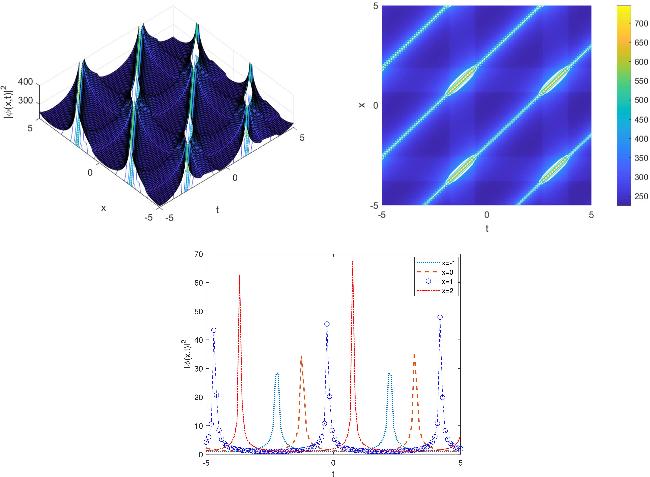
Figure 1. 3D, 2D and Contour plot of ( |
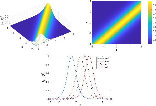
Figure 2. 3D, 2D and Contour plot of ( |
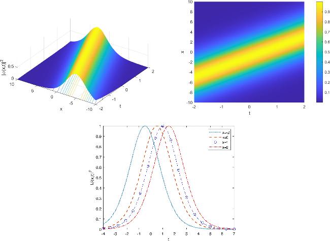
Figure 3. 3D, 2D and Contour plot of ( |
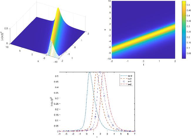
Figure 4. 3D, 2D and Contour plot of ( |
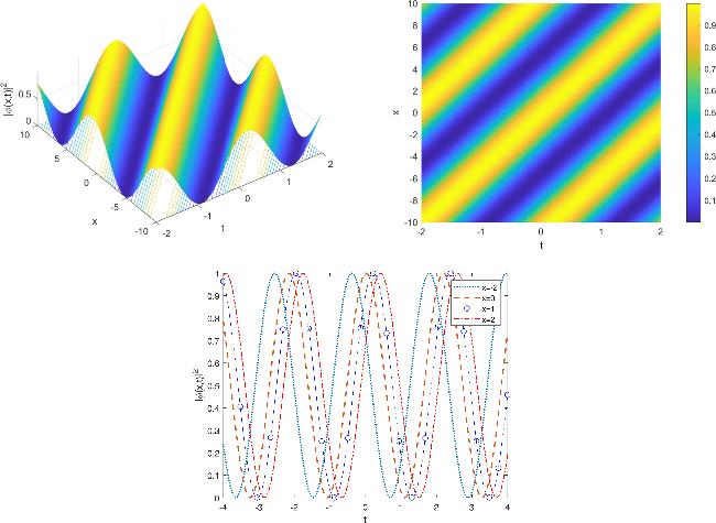


Figure 5. 3D, 2D and Contour plot of ( |
The novelty of this study is twofold and represents a fundamental shift in the paradigm of analytical solution methods for nonlinear PDEs. First, to the best of our knowledge, this work constitutes the first application of a variable coefficient sub-equation method to the CGLE, marking a clear departure from traditional approaches, which are universally constrained by the use of constant coefficient ODEs. This methodological innovation facilitates the exploration of a significantly broader solution space, thereby enabling the modeling of physical systems characterized by non-uniform or spatially varying properties. Second, the transition from constant to variable coefficients fundamentally alters the mathematical structure of the problem. Whereas conventional methodologies reduce the governing equations to a tractable system of algebraic equations, our approach yields a system of DAEs. The resolution of this DAE system serves as the key mechanism for introducing functional parameters into the solutions, resulting in new families of soliton forms that have not been previously documented in the literature. These generalized solutions possess significant potential for application across various scientific domains, including nonlinear optics for the description of pulse propagation in non-uniform fibers, fluid dynamics for the analysis of wave packets over variable topographies, and plasma physics for the study of localized waves in inhomogeneous media. By transcending the inherent constraints of constant-coefficient algebra, this work not only contributes new analytical results but also establishes a more powerful and versatile framework for investigating complex nonlinear models in non-uniform environments.
6. Conclusion
In this study, we introduced the VCSDGAE as a novel analytical approach to solving the CGLE, particularly in the context of anti-cubic nonlinearity. By moving away from conventional methods that typically employ constant coefficient ODEs and auxiliary ODEs, our method demonstrates a significant advancement in tackling nonlinear partial differential equations. The use of variable coefficient ODEs within a sub-equation framework not only enhances the adaptability of our approach but also allows for the derivation of precise analytical solutions to the CGLE. The stability of the obtained soliton solutions has been verified through linear stability analysis, confirming their robustness against small perturbations and establishing the parameter conditions required for their sustainable propagation.
The effectiveness and efficiency of this method were clearly illustrated through various examples, demonstrating its potential as a robust tool for addressing complex problems in fluid dynamics and wave propagation. Furthermore, our findings contribute to the broader landscape of analytical techniques available for mathematical physics, offering new pathways for researchers to explore solutions to challenging nonlinear equations. While the present work focuses on the analytical derivation and linear stability of soliton solutions, a more detailed investigation of their propagation characteristics, parameter dependence, and physical significance through numerical simulations and experimental validation is planned for future work.
Declarations
Conflicts of interest
The authors declare that there are no conflicts of interest associated with this publication.
Funding
Not applicable.
Data Availability Statement
All datasets utilized in this study are fully presented within the body of the manuscript.
Declaration of generative AI and AI-assisted technologies in the writing process
During the preparation of this work the author used ChatGPT in order to improve the readability and language of the manuscript. After using this tool/service, the author reviewed and edited the content as needed and takes full responsibility for the content of the published article.