Welcome to visit Communications in Theoretical Physics,
Quantum Physics and Quantum Information

Tighter Rényi-α entropy entanglement monogamy and polygamy relations of qubit systems

  • Wen Zhou , 1 ,
  • Zhong-Xi Shen , 2 ,
  • Dong-Ping Xuan , 1 ,
  • Zhi-Xi Wang , 1 ,
  • Shao-Ming Fei , 1, *
Expand
  • 1School of Mathematical Sciences, Capital Normal University, Beijing 100048, China
  • 2School of Mathematics and Physics, Nanyang Institute of Technology, Nanyang 473004, China

*Author to whom any correspondence should be addressed.

Received date: 2025-09-22

  Accepted date: 2026-02-27

  Online published: 2026-03-25

Copyright

© 2026 Institute of Theoretical Physics CAS, Chinese Physical Society and IOP Publishing. All rights, including for text and data mining, AI training, and similar technologies, are reserved.
This article is available under the terms of the IOP-Standard License.

Abstract

The monogamy and polygamy relations characterize the distributions of quantum entanglement in multipartite systems. We investigate the monogamy relations related to the Rényi-α entanglement (RαE) and polygamy relations related to the RαE of assistance (RαEoA). We present new entanglement monogamy relations satisfied by the η-th (η ≥ 2) power of RαE for α ≥ 2, and by the γ-th (γ ≥ 4) power of RαE for $\frac{\sqrt{7}-1}{2}\,\leqslant \,\alpha \lt 2$, respectively. Moreover, we present polygamy relations satisfied by the tth power of RαEoA with $\frac{\sqrt{7}-1}{2}\,\leqslant \,\alpha \lt \frac{\sqrt{13}-1}{2}$ for 0 ≤ t ≤ 1. We also give relationships among the residual entanglements of RαE and RαEoA, and the three tangle based on our general monogamy relations.

Cite this article

Wen Zhou , Zhong-Xi Shen , Dong-Ping Xuan , Zhi-Xi Wang , Shao-Ming Fei . Tighter Rényi-α entropy entanglement monogamy and polygamy relations of qubit systems[J]. Communications in Theoretical Physics, 2026 , 78(6) : 065102 . DOI: 10.1088/1572-9494/ae4b16

1. Introduction

Quantum entanglement is a pivotal aspect within quantum mechanics, yielding a comprehensive comprehension of quantum correlations' fundamental nature and being instrumental in the field of quantum information processing. As a fundamental resource for quantum tasks, quantum entanglement has been harnessed in a variety of quantum communication protocols, including superdense coding [1], quantum cryptography [2], quantum teleportation [3] and remote-state preparation [4].
A fundamental characteristic of quantum entanglement is illustrated by the monogamy relation [5]. This principle states that a quantum subsystem, when entangled with one of the other subsystems, restricts its level of entanglement with the rest, a notion known as the monogamy of entanglement (MoE) [5]. Consider a three-qubit system where Alice and Bob share a Bell state $| {\rm{\Psi }}\rangle =\frac{1}{\sqrt{2}}(| 00\rangle +| 11\rangle )$ across systems A and B, they are precluded from sharing any entangled states with Charlie's system C in this scenario. Such inherent restricted entanglement distribution can be exploited in the realm of quantum cryptography, enabling the estimation of the amount of information that an eavesdropper might intercept about the secret key that is intended to be securely shared [6]. MoE has been extensively utilized in diverse disciplines such as condensed-matter physics [7] and even black-hole physics [8]. It highlights the concept that entanglement is not freely distributed, leading to profound implications for the manipulation and distribution of quantum information in multipartite quantum systems [9, 10]. Mathematically, the MoE is expressed by utilizing an entanglement measure denoted as ${ \mathcal E }$, applied to a tripartite system ϱABC, as follows
$\begin{eqnarray}{ \mathcal E }({\varrho }_{A| BC})\geqslant { \mathcal E }({\varrho }_{AB})+{ \mathcal E }({\varrho }_{AC}),\end{eqnarray}$
which is commonly recognized as the CKW inequality [5], where ${\varrho }_{AB}={{\rm{Tr}}}_{C}({\varrho }_{ABC})$, ${\varrho }_{AC}={{\rm{Tr}}}_{B}({\varrho }_{ABC})$, and ${ \mathcal E }$ serves as a quantum entanglement measure. It has been further shown that the squared concurrence satisfies the monogamy relations for multi-qubit states [5]. Subsequently, the monogamy relations have been extensively studied for other entanglement measures such as entanglement of formation [11], entanglement negativity [12], the Tsallis-q entanglement, and Rényi-α entanglement (RαE) [13, 14].
Dual to the entanglement measures, the concept of entanglement of assistances leads to polygamy relations. Gour et al introduced in [15] the initial polygamy inequality for arbitrary tripartite systems, which is based on the squared concurrence of assistance. The polygamy relation for the tripartite state ϱABC is defined by
$\begin{eqnarray}{{ \mathcal E }}_{a}({\varrho }_{A| BC})\leqslant {{ \mathcal E }}_{a}({\varrho }_{A| B})+{{ \mathcal E }}_{a}({\varrho }_{A| C}),\end{eqnarray}$
where ${{ \mathcal E }}_{a}$ represents the entanglement measure of assistance that corresponds to ${ \mathcal E }$. Subsequently, Buscemi et al in [16] introduced a polygamy relation for any dimensional pure states. Later, Kim extended this relationship to the case of arbitrary dimensional mixed states [17].
As a kind of generalized entanglement of formation [18], the RαE has the advantages to characterize quantum phases with differing computational power [19], as well as the topologically ordered states [20, 21]. It is naturally of significance to study the monogamy and polygamy relations associated with RαE and its dual RαE of assistance (RαEoA) in multipartite systems. Recently, it was demonstrated that if α ≥ 2, the RαE satisfies the monogamy relation within multi-qubit systems [22]. In general, enhancing monogamy relations allows for a more accurate depiction of multipartite entanglement. Subsequently, more tighter monogamous relations have been presented for RαE [2327]. In [28], Song et al presented a novel polygamy relation of multipartite systems using RαEoA for $\frac{\sqrt{7}-1}{2}\,\leqslant \,\alpha \lt \frac{\sqrt{13}-1}{2}$. Then, in [23] the authors further improved the polygamy inequalities.
The following sections detail the organization of this article. In section 2, we will review the essential foundational concepts required. In section 3, we focus on tightening the monogamy relations satisfied by the η-th (η ≥ 2) power of RαE for α ≥ 2, and by the γ-th (γ ≥ 4) power of RαE for $\frac{\sqrt{7}-1}{2}\,\leqslant \,\alpha \lt 2$, respectively. The results indicate that the newly derived monogamy relations exhibit tighter bounds than the ones given in [2227]. In section 4, we give the polygamy relations satisfied by the t-th power of RαEoA with $\frac{\sqrt{7}-1}{2}\,\leqslant \,\alpha \lt \frac{\sqrt{13}-1}{2}$ for 0 ≤ t ≤ 1, which are tighter than those given in [23, 28]. In section 5, we present a bound of RαEoA by examining the relations between the residual entanglement of RαE and the three tangle. In addition, we provide detailed examples to illustrate the benefits of our results. The conclusion is given in section 6.

2. Preliminaries

Let HA and HB represent finite dimensional complex Hilbert spaces corresponding to the quantum subsystems A and B, respectively. For a bipartite pure state ∣ψAB ∈ HA ⨂ HB,  the concurrence ${\mathscr{C}}(| \psi {\rangle }_{AB})$ is expressed as [29, 30]
$\begin{eqnarray}{\mathscr{C}}(| \psi {\rangle }_{AB})=\sqrt{2[1-{\rm{Tr}}({\varrho }_{A}^{2})]},\end{eqnarray}$
where ${\varrho }_{A}={{\rm{Tr}}}_{B}(| \psi {\rangle }_{AB}\langle \psi | )$. The concurrence of a bipartite mixed state ϱAB ∈ HA ⨂ HB is derived via the convex roof extension,
$\begin{eqnarray}{\mathscr{C}}({\varrho }_{AB})=\mathop{\min }\limits_{\{{p}_{i},| {\psi }_{i}\rangle \}}\displaystyle \sum _{i}{p}_{i}{\mathscr{C}}(| {\psi }_{i}\rangle ),\end{eqnarray}$
where the minimum is taken over all possible pure decompositions of ϱAB = ∑ipiψiABψi∣ with pi ≥ 0 and ∑ipi = 1.
For an N-qubit state $| \psi {\rangle }_{A{B}_{1}\cdots {B}_{N-1}}\in {H}_{A}\otimes {H}_{{B}_{1}}\otimes \cdots \otimes {H}_{{B}_{N-1}}$, the concurrence ${\mathscr{C}}(| \psi {\rangle }_{A| {B}_{1}\cdots {B}_{N-1}})$ for the state $| \psi {\rangle }_{A{B}_{1}\cdots {B}_{N-1}}$ under the bipartite partition A and B1B2 ⋯ BN−1 obeys the following monogamy inequality [6],
$\begin{eqnarray}\begin{array}{r}{{\mathscr{C}}}^{2}(| \psi {\rangle }_{A| {B}_{1}{B}_{2}\cdots {B}_{N-1}})\geqslant \displaystyle \sum _{i=1}^{N-1}{{\mathscr{C}}}^{2}({\varrho }_{A| {B}_{i}}),\end{array}\end{eqnarray}$
where ${\mathscr{C}}({\varrho }_{A| {B}_{i}})$ is the concurrence of the reduced state ${\varrho }_{A{B}_{i}}={{\rm{tr}}}_{{B}_{1}\cdots {B}_{i-1}{B}_{i+1}\cdots {B}_{N-1}}(\varrho )$.
For a tripartite pure state ∣ψABC, the concurrence of assistance is expressed as [31, 32],
$\begin{eqnarray*}\begin{array}{r}{{\mathscr{C}}}_{a}(| \psi {\rangle }_{ABC})\equiv {{\mathscr{C}}}_{a}({\varrho }_{AB})=\mathop{\max }\limits_{\{{p}_{i},| {\psi }_{i}\rangle \}}\displaystyle \sum _{i}{p}_{i}{\mathscr{C}}(| {\psi }_{i}\rangle ),\end{array}\end{eqnarray*}$
where the maximum is taken over all possible pure state decompositions of ${\varrho }_{AB}={{\rm{Tr}}}_{C}(| \psi {\rangle }_{ABC}{\langle \psi | )={\sum }_{i}{p}_{i}| {\psi }_{i}\rangle }_{AB}\langle {\psi }_{i}| $ with pi ≥ 0 and ∑ipi = 1. For a pure state ϱAB, it holds that ${\mathscr{C}}(| \psi {\rangle }_{AB})={{\mathscr{C}}}_{a}({\varrho }_{AB})$.
For a two-qubit mixed state ϱ, the concurrence of ϱ is expressed as [33]
$\begin{eqnarray*}\begin{array}{r}{\mathscr{C}}(\varrho )=\max \{{\vartheta }_{1}-{\vartheta }_{2}-{\vartheta }_{3}-{\vartheta }_{4},0\},\end{array}\end{eqnarray*}$
where ϑ1ϑ2ϑ3ϑ4 represents the eigenvalues of the matrix $\sqrt{\sqrt{\varrho }\widetilde{\varrho }\sqrt{\varrho }}$. The expression $\widetilde{\varrho }$ is defined as (ϱy ⨂ ϱy)ϱ*(ϱy ⨂ ϱy), with ϱ* denoting the complex conjugation of ϱ, and ϱy denoting the standard Pauli matrix.
RαE is a widely recognized entanglement measure that has found numerous applications in various fields such as condensed matter physics [34]. For a bipartite pure state ∣φAB, the RαE is defined as [22]
$\begin{eqnarray}{R}_{\alpha }(| \varphi {\rangle }_{AB})=\frac{1}{1-\alpha }{{\rm{log}}}_{2}({\rm{Tr}}{\varrho }_{A}^{\alpha }),\end{eqnarray}$
where α > 0, α ≠ 1 and ${\varrho }_{A}={{\rm{Tr}}}_{B}(| \varphi {\rangle }_{AB}\langle \varphi | )$. When α tends to 1, the RαE converges to the von Neumann entropy. The RαE of a bipartite mixed state ϱAB is defined by
$\begin{eqnarray}{R}_{\alpha }({\varrho }_{AB})={\rm{\min }}\displaystyle \sum _{i}{p}_{i}{R}_{\alpha }(| {\varphi }_{i}{\rangle }_{AB}),\end{eqnarray}$
where the minimum is taken over all possible pure state decompositions $\{{p}_{i},{\varphi }_{AB}^{i}\}$ of ϱAB.
It has been proved in [22, 35] that when $\alpha \,\geqslant \,\frac{\sqrt{7}-1}{2}$, the RαE of any two-qubit state ϱAB has an analytical formula,
$\begin{eqnarray}{R}_{\alpha }({\varrho }_{AB})={f}_{\alpha }({\mathscr{C}}({\varrho }_{AB})),\end{eqnarray}$
where
$\begin{eqnarray}\begin{array}{rcl}{f}_{\alpha }(\xi ) & = & \frac{1}{1-\alpha }{{\rm{log}}}_{2}\left[{\left(\frac{1-\sqrt{1-{\xi }^{2}}}{2}\right)}^{\alpha }\right.\\ & & \left.+{\left(\frac{1+\sqrt{1-{\xi }^{2}}}{2}\right)}^{\alpha }\right]\end{array}\end{eqnarray}$
is a monotonically increasing convex function, 0 ≤ ξ ≤ 1. When α ≥ 2, one has [22],
$\begin{eqnarray}\begin{array}{r}{f}_{\alpha }(\sqrt{{\xi }_{1}^{2}+{\xi }_{2}^{2}})\geqslant {f}_{\alpha }({\xi }_{1})+{f}_{\alpha }({\xi }_{2}),\end{array}\end{eqnarray}$
for $0\,\leqslant \,{\xi }_{1},{\xi }_{2},{\xi }_{1}^{2}+{\xi }_{2}^{2}\,\leqslant \,1$. When $\frac{\sqrt{7}-1}{2}\,\leqslant \,\alpha \lt 2$, it has been shown that [26],
$\begin{eqnarray}{f}_{\alpha }^{2}(\sqrt{{\xi }_{1}^{2}+{\xi }_{2}^{2}})\geqslant {f}_{\alpha }^{2}({\xi }_{1})+{f}_{\alpha }^{2}({\xi }_{2}),\end{eqnarray}$
for $0\,\leqslant \,{\xi }_{1},{\xi }_{2},{\xi }_{1}^{2}+{\xi }_{2}^{2}\,\leqslant \,1$.
For any N-qubit state ${\varrho }_{A{B}_{1}\cdots {B}_{N-1}}\in {H}_{A}\otimes {H}_{{B}_{1}}\otimes \cdots \otimes {H}_{{B}_{N-1}}$, RαE satisfies the following monogamy relation [22],
$\begin{eqnarray}{R}_{\alpha }^{\mu }\left({\varrho }_{A| {B}_{1}\cdots {B}_{N-1}}\right)\geqslant {R}_{\alpha }^{\mu }\left({\varrho }_{A| {B}_{1}}\right)+\cdots +{R}_{\alpha }^{\mu }\left({\varrho }_{A| {B}_{N-1}}\right),\end{eqnarray}$
for α ≥ 2 and μ ≥ 1, and the following monogamy relation [26],
$\begin{eqnarray}{R}_{\alpha }^{\omega }\left({\varrho }_{A| {B}_{1}\cdots {B}_{N-1}}\right)\geqslant {R}_{\alpha }^{\omega }\left({\varrho }_{A| {B}_{1}}\right)+\cdots +{R}_{\alpha }^{\omega }\left({\varrho }_{A| {B}_{N-1}}\right),\end{eqnarray}$
for $\alpha \,\geqslant \,\frac{\sqrt{7}-1}{2}$ and ω ≥ 2, where ${R}_{\alpha }\left({\varrho }_{A| {B}_{1}\cdots {B}_{N-1}}\right)$ is the RαE of ${\varrho }_{A{B}_{1}\cdots {B}_{N-1}}$ related to the bipartition A and the rest, and ${R}_{\alpha }\left({\varrho }_{A| {B}_{i-1}}\right)$ is the RαE of the reduced density matrix ${\varrho }_{A{B}_{i-1}}$ of the two-qubit system ABi−1, i = 2, …, n.
Dual to RαE, the RαEoA is expressed as
$\begin{eqnarray}{R}_{\alpha }^{a}({\varrho }_{AB})={\rm{\max }}\displaystyle \sum _{i}{p}_{i}{R}_{\alpha }(| {\varphi }_{i}{\rangle }_{AB}),\end{eqnarray}$
where the maximum is taken over all possible pure state decompositions $\{{p}_{i},{\varphi }_{AB}^{i}\}$ of ϱAB. For $\frac{\sqrt{7}-1}{2}\,\leqslant \,\alpha \,\leqslant \,\frac{\sqrt{13}-1}{2}$, 0 ≤ t ≤ 1 and any N-qubit state ${\varrho }_{A{B}_{1}\cdots {B}_{N-1}}$, one has [28]
$\begin{eqnarray}{({R}_{\alpha }^{a})}^{t}\left({\varrho }_{A| {B}_{1}\cdots {B}_{N-1}}\right)\leqslant {({R}_{\alpha }^{a})}^{t}\left({\varrho }_{A| {B}_{1}}\right)+\cdots +{({R}_{\alpha }^{a})}^{t}\left({\varrho }_{A| {B}_{N-1}}\right),\end{eqnarray}$
where ${R}_{\alpha }^{a}\left({\varrho }_{A| {B}_{1}\cdots {B}_{N-1}}\right)$ denotes the RαEoA in the partition AB1 ⋯ BN−1, and ${R}_{\alpha }^{a}\left({\varrho }_{A| {B}_{i-1}}\right)$ is the RαEoA of the reduced density matrix ${\varrho }_{A{B}_{i-1}}$ of the two-qubit system ABi−1,i = 2, …, n.

3. Tighter monogamy relations for RαE

Monogamy relations serve as a pivotal tool in advancing our comprehension of entanglement distribution within multipartite systems. Tighter monogamy relations enable a more detailed delineation of the distribution of quantum correlations within the subsystems. This could result in tighter security constraints within the realm of quantum cryptography [36]. In the following, we establish new classes of tighter monogamy relations of RαE. We first introduce some related lemmas.

[37] For λ≥2 and ς≥0, one has

$\begin{eqnarray}\begin{array}{l}{(1+\varsigma )}^{\lambda -1}\geqslant 1+(\lambda -1)\varsigma .\end{array}\end{eqnarray}$

For 0 ≤ θ ≤ 1 and λ≥2, we see that

$\begin{eqnarray}\begin{array}{l}{(1+\theta )}^{\lambda }\geqslant 1+\lambda \theta +({2}^{\lambda }-\lambda -1){\theta }^{\lambda }.\end{array}\end{eqnarray}$

If θ = 0, the inequality holds. If θ ≠ 0, the core idea is to reformulate the desired inequality. Observing that equation (17) is equivalent to $\frac{{(1+\theta )}^{\lambda }-\lambda \theta -1}{{\theta }^{\lambda }}\,\geqslant \,{2}^{\lambda }-\lambda -1$, we consider the function $f(\theta ,\lambda )=\frac{{(1+\theta )}^{\lambda }-\lambda \theta -1}{{\theta }^{\lambda }}$ for 0 < θ ≤ 1. Proving the inequality (17) is now equivalent to showing f(θλ) ≥ f(1, λ) = 2λ − λ − 1. To establish this, we examine the monotonicity of f with respect to θ. We have

$\begin{eqnarray*}\begin{array}{l}\frac{\partial f}{\partial \theta }=\frac{\lambda {\theta }^{\lambda -1}\{[{(1+\theta )}^{\lambda -1}-1]\theta -[{(1+\theta )}^{\lambda }-\lambda \theta -1]\}}{{\theta }^{2\lambda }}\\ =\,\frac{[\lambda {(1+\theta )}^{\lambda -1}-\lambda ]{\theta }^{\lambda }-\left[{(1+\theta )}^{\lambda }-\lambda \theta -1\right]\lambda {\theta }^{\lambda -1}}{{\theta }^{2\lambda }}\\ =\,\frac{\lambda {\theta }^{\lambda -1}[1+(\lambda -1)\theta -{(1+\theta )}^{\lambda -1}]}{{\theta }^{2\lambda }}.\end{array}\end{eqnarray*}$
By lemma 1, this implies g(θ) = (1 + θ)λ − λθ − 1 ≤ 0. Thus, $\frac{\partial f}{\partial \theta }\,\leqslant \,0$ for all 0 < θ ≤ 1. The function f(θλ) decreases with respect to θ. Since 0 ≤ θ ≤ 1, f(θλ) ≥ f(1, λ) = 2λ − λ − 1. Multiplying both sides by the positive quantity θλ we obtain the inequality (17), (1 + θ)λ ≥ 1 + λθ + (2λ − λ − 1)θλ. This completes the proof.  □

We present below the tighter monogamy inequality in terms of the RαE for α ≥ 2.

For any tripartite quantum state ϱABC, we have for α ≥ 2 and η ≥ 2,

(1) If Rα(ϱA∣B) ≥ Rα(ϱA∣C), then

$\begin{eqnarray}\begin{array}{rcl}{R}_{\alpha }^{\eta }({\varrho }_{A| BC}) & \geqslant & {R}_{\alpha }^{\eta }({\varrho }_{A| B})+\eta {R}_{\alpha }^{\eta -1}({\varrho }_{A| B}){R}_{\alpha }({\varrho }_{A| C})\\ & & +({2}^{\eta }-\eta -1){R}_{\alpha }^{\eta }({\varrho }_{A| C}).\end{array}\end{eqnarray}$
(2) If Rα(ϱAB) ≤ Rα(ϱAC), then
$\begin{eqnarray}\begin{array}{rcl}{R}_{\alpha }^{\eta }({\varrho }_{A| BC}) & \geqslant & {R}_{\alpha }^{\eta }({\varrho }_{A| C})+\eta {R}_{\alpha }^{\eta -1}({\varrho }_{A| C}){R}_{\alpha }({\varrho }_{A| B})\\ & & +({2}^{\eta }-\eta -1){R}_{\alpha }^{\eta }({\varrho }_{A| B}).\end{array}\end{eqnarray}$

If Rα(ϱAB) ≥ Rα(ϱAC), we have

$\begin{eqnarray}\begin{array}{rcl}{R}_{\alpha }^{\eta }({\varrho }_{A| BC}) & \geqslant & {[{R}_{\alpha }({\varrho }_{A| B})+{R}_{\alpha }({\varrho }_{A| C})]}^{\eta }\\ & = & {R}_{\alpha }^{\eta }({\varrho }_{A| B}){\left(1+\frac{{R}_{\alpha }({\varrho }_{A| C})}{{R}_{\alpha }({\varrho }_{A| B})}\right)}^{\eta }\\ & \geqslant & {R}_{\alpha }^{\eta }({\varrho }_{A| B})+\eta {R}_{\alpha }^{\eta -1}({\varrho }_{A| B}){R}_{\alpha }({\varrho }_{A| C})\\ & & +({2}^{\eta }-\eta -1){R}_{\alpha }^{\eta }({\varrho }_{A| C}),\end{array}\end{eqnarray}$
where the first inequality is derived from the inequality (12), and the second inequality is due to the inequality (17) in lemma 2. The inequality (19) can be proved in a similar way.  □

From lemma 2, we have

$\begin{eqnarray*}\begin{array}{rcl}{(1+\theta )}^{\lambda } & \geqslant & 1+\lambda \theta +({2}^{\lambda }-\lambda -1){\theta }^{\lambda }\\ & \geqslant & 1+\frac{{\lambda }^{2}}{\lambda +1}\theta +({2}^{\lambda }-\frac{{\lambda }^{2}}{\lambda +1}-1){\theta }^{\lambda }\\ & & (\,\rm{The inequality in [27]}\,)\\ & \geqslant & 1+\frac{\lambda }{2}\theta +({2}^{\lambda }-\frac{\lambda }{2}-1){\theta }^{\lambda }\\ & & \quad (\,\rm{The inequality in [26]}\,)\\ & \geqslant & 1+({2}^{\lambda }-1){\theta }^{\lambda }\quad (\,\rm{The inequality in [25]}\,).\end{array}\end{eqnarray*}$
Since $\lambda \gt \frac{{\lambda }^{2}}{\lambda +1}\,\geqslant \,\frac{\lambda }{2}$, θ − θλ > 0 for 0 ≤ θ ≤ 1 and λ ≥ 2, obviously our inequality given in theorem 1 is tighter than the ones presented in [2225].

Generalizing theorem 1 to N-qubit quantum systems, we obtain the following theorem. The conditions in theorem 2 describe the distribution order of entanglement among the subsystems: the first z subsystems (i.e. B1 to Bz, ∀ 1 ≤ zN − 3, N ≥ 4) have strong entanglement with subsystem A, sufficient to dominate the combined entanglement of all subsequent subsystems; starting from Bz+1, the entanglement is weaker and cannot dominate the subsequent parts. This ordering allows us to iteratively simplify the derivation of the monogamy inequality, ensuring a tighter bound.

For any N-qubit quantum state ${\varrho }_{A{B}_{1}\cdots {B}_{N-1}}\in {H}_{A}\otimes {H}_{{B}_{1}}\otimes \cdots \otimes {H}_{{B}_{N-1}}$, if ${R}_{\alpha }({\varrho }_{A| {B}_{i}})\,\geqslant \,\displaystyle {\sum }_{l=i+1}^{N-1}{R}_{\alpha }({\varrho }_{A| {B}_{l}})$ for i = 1, 2, ⋯  , z, and ${R}_{\alpha }({\varrho }_{A| {B}_{j}})\,\leqslant \,\displaystyle {\sum }_{l=j+1}^{N-1}{R}_{\alpha }({\varrho }_{A| {B}_{l}})$ for j = z + 1, ⋯  , N − 2, ∀ 1 ≤ zN − 3, N ≥ 4, then

$\begin{array}{l}R_{\alpha}^{\eta}\left(\varrho_{A \mid B_{1} \cdots B_{N-1}}\right) \\\geqslant \sum_{i=1}^{z}\left\{( 2 ^ { \eta } - \eta - 1 ) ^ { i - 1 } \left[R_{\alpha}^{\eta}\left(\varrho_{A \mid B_{i}}\right)\right.\right. \\\left.\left.+\eta R_{\alpha}^{\eta-1}\left(\varrho_{A \mid B_{i}}\right)\left(\sum_{l=i+1}^{N-1} R_{\alpha}\left(\varrho_{A \mid B_{l}}\right)\right)\right]\right\} \\+\left(2^{\eta}-\eta-1\right)^{z}\left(2^{\eta}-1\right)\left[R_{\alpha}^{\eta}\left(\varrho_{A \mid B_{z+1}}\right)\right. \\\left.+\cdots+R_{\alpha}^{\eta}\left(\varrho_{A \mid B_{N-3}}\right)\right] \\+\left(2^{\eta}-\eta-1\right)^{z}\left\{\left(2^{\eta}-\eta-1\right) R_{\alpha}^{\eta}\left(\varrho_{A \mid B_{N-2}}\right)\right. \\\left.+\eta R_{\alpha}\left(\varrho_{A \mid B_{N-2}}\right) R_{\alpha}^{\eta-1}\left(\varrho_{A \mid B_{N-1}}\right)+R_{\alpha}^{\eta}\left(\varrho_{A \mid B_{N-1}}\right)\right\}\end{array}$
where η ≥ 2 and α ≥ 2.

When ${R}_{\alpha }({\varrho }_{A| {B}_{i}})\,\geqslant \,\displaystyle {\sum }_{l=i+1}^{N-1}{R}_{\alpha }({\varrho }_{A| {B}_{l}})$ for i = 1, 2, ⋯  , z, set ${\theta }_{i}=\displaystyle {\sum }_{l=i+1}^{N-1}{R}_{\alpha }({\varrho }_{A| {B}_{l}})/{R}_{\alpha }({\varrho }_{A| {B}_{i}})$. Substituting θi into the inequality (17) and using inequality (12), we get

$\begin{eqnarray}\begin{array}{rcl}{R}_{\alpha }^{\eta }({\varrho }_{A| {B}_{i}\cdots {B}_{N-1}}) & \geqslant & {\left(\displaystyle \sum _{l=i}^{N-1}{R}_{\alpha }({\varrho }_{A| {B}_{l}})\right)}^{\eta }\\ & \geqslant & {R}_{\alpha }^{\eta }({\varrho }_{A| {B}_{i}})+\eta {R}_{\alpha }^{\eta -1}({\varrho }_{A| {B}_{i}})\\ & & \times \displaystyle \sum _{l=i+1}^{N-1}{R}_{\alpha }({\varrho }_{A| {B}_{l}})+({2}^{\eta }-\eta -1)\\ & & \times \left(\displaystyle \sum _{l=i+1}^{N-1}{R}_{\alpha }({\varrho }_{A| {B}_{l}})\right).\end{array}\end{eqnarray}$
When i = 1, we obtain
$\begin{eqnarray}\begin{array}{l}{R}_{\alpha }^{\eta }({\varrho }_{A| {B}_{1}\cdots {B}_{N-1}})\\ \geqslant \,{R}_{\alpha }^{\eta }({\varrho }_{A| {B}_{1}})+\eta {R}_{\alpha }^{\eta -1}({\varrho }_{A| {B}_{1}})\left(\displaystyle \sum _{l=2}^{N-1}{R}_{\alpha }({\varrho }_{A| {B}_{l}})\right)\\ +\,({2}^{\eta }-\eta -1){\left(\displaystyle \sum _{l=2}^{N-1}{R}_{\alpha }({\varrho }_{A| {B}_{l}})\right)}^{\eta }\\ \geqslant \,{R}_{\alpha }^{\eta }({\varrho }_{A| {B}_{1}})+\eta {R}_{\alpha }^{\eta -1}({\varrho }_{A| {B}_{1}})\left(\displaystyle \sum _{l=2}^{N-1}{R}_{\alpha }({\varrho }_{A| {B}_{l}})\right)\\ +\,({2}^{\eta }-\eta -1){R}_{\alpha }^{\eta }({\varrho }_{A| {B}_{2}})\\ +\,({2}^{\eta }-\eta -1)\eta {R}_{\alpha }^{\eta -1}({\varrho }_{A| {B}_{2}})\left(\displaystyle \sum _{l=3}^{N-1}{R}_{\alpha }({\varrho }_{A| {B}_{l}})\right)\\ +\,{({2}^{\eta }-\eta -1)}^{2}{\left(\displaystyle \sum _{l=3}^{N-1}{R}_{\alpha }({\varrho }_{A| {B}_{l}})\right)}^{\eta }\\ \geqslant \,\cdots \\ \geqslant \,\displaystyle \sum _{i=1}^{z}\left\{{({2}^{\eta }-\eta -1)}^{i-1}\left[{R}_{\alpha }^{\eta }({\varrho }_{A| {B}_{i}})\right.\right.\\ \left.\left.+\,\eta {R}_{\alpha }^{\eta -1}({\varrho }_{A| {B}_{i}})\left(\displaystyle \sum _{l=i+1}^{N-1}{R}_{\alpha }({\varrho }_{A| {B}_{l}})\right)\right]\right\}\\ +\,{({2}^{\eta }-\eta -1)}^{z}{\left(\displaystyle \sum _{l=z+1}^{N-1}{R}_{\alpha }({\varrho }_{A| {B}_{l}})\right)}^{\eta },\end{array}\end{eqnarray}$
by utilizing the inequality (22) iteratively.

When ${R}_{\alpha }({\varrho }_{A| {B}_{j}})\,\leqslant \,\displaystyle {\sum }_{l=j+1}^{N-1}{R}_{\alpha }({\varrho }_{A| {B}_{l}})$ for j = z + 1, ⋯  , N − 2, we use a strengthened version of lemma 2. Noting that for 0 ≤ θ ≤ 1 and λ ≥ 2, we have 1 + λθ + (2λ − λ − 1)θλ ≥1 + (2λ − 1)θλ. This implies (1 + θ)λ ≥ 1 + (2λ − 1)θλ. Let ${\theta }_{j}={R}_{\alpha }({\varrho }_{A| {B}_{j}})/\displaystyle {\sum }_{l=j+1}^{N-1}{R}_{\alpha }({\varrho }_{A| {B}_{l}})$. Substituting θj into the above inequality, we obtain

$\begin{eqnarray}\begin{array}{rcl}{\left(\displaystyle \sum _{l=j}^{N-1}{R}_{\alpha }({\varrho }_{A| {B}_{l}})\right)}^{\eta } & \geqslant & {\left(\displaystyle \sum _{l=j+1}^{N-1}{R}_{\alpha }({\varrho }_{A| {B}_{l}})\right)}^{\eta }\\ & & +({2}^{\eta }-1){R}_{\alpha }^{\eta }({\varrho }_{A| {B}_{j}}).\end{array}\end{eqnarray}$
When j = z + 1, we see that
$\begin{eqnarray}\begin{array}{l}{\left(\displaystyle \sum _{l=z+1}^{N-1}{R}_{\alpha }({\varrho }_{A| {B}_{l}})\right)}^{\eta }\\ \geqslant \,{\left(\displaystyle \sum _{l=z+2}^{N-1}{R}_{\alpha }({\varrho }_{A| {B}_{l}})\right)}^{\eta }+({2}^{\eta }-1){R}_{\alpha }^{\eta }({\varrho }_{A| {B}_{z}+1})\\ \geqslant \,{[{R}_{\alpha }({\varrho }_{A| {B}_{N-2}})+{R}_{\alpha }({\varrho }_{A| {B}_{N-1}})]}^{\eta }\\ +\,({2}^{\eta }-1)[{R}_{\alpha }^{\eta }({\varrho }_{A| {B}_{z+1}})+\cdots +{R}_{\alpha }^{\eta }({\varrho }_{A| {B}_{N-3}})]\\ \geqslant \,{R}_{\alpha }^{\eta }({\varrho }_{A| {B}_{N-1}})+\eta {R}_{\alpha }({\varrho }_{A| {B}_{N-2}}){R}_{\alpha }^{\eta -1}({\varrho }_{A| {B}_{N-1}})\\ +\,({2}^{\eta }-\eta -1){R}_{\alpha }^{\eta }({\varrho }_{A| {B}_{N-2}})\\ +\,({2}^{\eta }-1)[{R}_{\alpha }^{\eta }({\varrho }_{A| {B}_{z+1}})+\cdots +{R}_{\alpha }^{\eta }({\varrho }_{A| {B}_{N-3}})],\end{array}\end{eqnarray}$
where the first and second inequalities hold because of the inequality (36), the third inequality is derived from the inequality (17). Combining (23) and (25), we get the inequality (21).  □

In particular, we have the following monogamy relation.

For any N-qubit quantum state ${\varrho }_{A{B}_{1}\cdots {B}_{N-1}}$ $\in {H}_{A}\otimes {H}_{{B}_{1}}\otimes $ $\cdots \otimes {H}_{{B}_{N-1}}$, if ${R}_{\alpha }({\varrho }_{A| {B}_{i}})\,\geqslant \,\displaystyle {\sum }_{l=i+1}^{N-1}{R}_{\alpha }({\varrho }_{A| {B}_{l}})$ for i = 1, 2, ⋯  , N − 2, then

$\begin{eqnarray}\begin{array}{rcl}{R}_{\alpha }^{\eta }({\varrho }_{A| {B}_{1}\cdots {B}_{N-1}}) & \geqslant & \displaystyle \sum _{i=1}^{N-2}\left\{{({2}^{\eta }-\eta -1)}^{i-1}\right.\\ & & \times \left[{R}_{\alpha }^{\eta }({\varrho }_{A| {B}_{i}})+\eta {R}_{\alpha }^{\eta -1}({\varrho }_{A| {B}_{i}})\right.\\ & & \left.\left.\times \left(\displaystyle \sum _{l=i+1}^{N-1}{R}_{\alpha }({\varrho }_{A| {B}_{l}})\right)\right]\right\}\\ & & +{({2}^{\eta }-\eta -1)}^{N-2}{R}_{\alpha }^{\eta }({\varrho }_{A| {B}_{N}-1}),\end{array}\end{eqnarray}$
where η ≥ 2 and α ≥ 2.

To illustrate the tightness of the monogamy inequality, we consider the following example.

Under local unitary operations, any three-qubit pure state can be written as [38, 39],
$\begin{eqnarray}\begin{array}{rcl}| \psi {\rangle }_{A| BC} & = & {\lambda }_{0}| 000\rangle +{\lambda }_{1}{{\rm{e}}}^{{\rm{i}}\varphi }| 100\rangle +{\lambda }_{2}| 101\rangle \\ & & +{\lambda }_{3}| 110\rangle +{\lambda }_{4}| 111\rangle ,\end{array}\end{eqnarray}$
where 0 ≤ φπ, λi ≥ 0, i = 0, 1, 2, 3, 4, and ${\sum }_{i=0}^{4}{\lambda }_{i}^{2}=1$. Set ${\lambda }_{0}=\frac{\sqrt{5}}{3}$, λ1 = 0, λ4 = 0, ${\lambda }_{2}=\frac{\sqrt{3}}{3}$ and ${\lambda }_{3}=\frac{1}{3}$. When α = 2, we get R2(ψABC) = 0.98230, R2(ϱAB) = 0.66742 and R2(ϱAC) = 0.19010. Thus,
$\begin{eqnarray}\begin{array}{r}{R}_{2}^{\eta }({\varrho }_{A| B})+({2}^{\eta }-\eta -1){R}_{2}^{\eta }({\varrho }_{A| C})\\ \quad +\,\eta {R}_{2}^{\eta -1}({\varrho }_{A| B}){R}_{2}({\varrho }_{A| C})\\ \quad =\,{(0.66742)}^{\eta }+\eta {(0.66742)}^{\eta -1}(0.19010)\\ \quad +\,({2}^{\eta }-\eta -1){(0.19010)}^{\eta },\end{array}\end{eqnarray}$
$\begin{eqnarray}\begin{array}{r}{R}_{2}^{\eta }({\varrho }_{A| B})+{R}_{2}^{\eta }({\varrho }_{A| C})={(0.66742)}^{\eta }+{(0.19010)}^{\eta },\end{array}\end{eqnarray}$
$\begin{eqnarray}\begin{array}{r}{R}_{2}^{\eta }({\varrho }_{A| B})+({2}^{\eta }-1){R}_{2}^{\eta }({\varrho }_{A| C})\\ \quad =\,{(0.66742)}^{\eta }+({2}^{\eta }-1){(0.19010)}^{\eta },\end{array}\end{eqnarray}$
$\begin{eqnarray}\begin{array}{r}{R}_{2}^{\eta }({\varrho }_{A| B})+\frac{\eta }{2}{R}_{2}^{\eta -1}({\varrho }_{A| B}){R}_{2}({\varrho }_{A| C})\\ \quad +({2}^{\eta }-\frac{\eta }{2}-1){R}_{2}^{\eta }({\varrho }_{A| C})\\ \quad =\,{(0.66742)}^{\eta }+\frac{\eta }{2}{(0.66742)}^{\eta -1}(0.19010)\\ \quad +\,({2}^{\eta }-\frac{\eta }{2}-1){(0.19010)}^{\eta },\end{array}\end{eqnarray}$
$\begin{eqnarray}\begin{array}{r}{R}_{2}^{\eta }({\varrho }_{A| B})+\frac{{\eta }^{2}}{\eta +1}{R}_{2}^{\eta -1}({\varrho }_{A| B}){R}_{2}({\varrho }_{A| C})\\ \quad +\,({2}^{\eta }-\frac{{\eta }^{2}}{\eta +1}-1){R}_{2}^{\eta }({\varrho }_{A| C})\\ \quad =\,{(0.66742)}^{\eta }+\frac{{\eta }^{2}}{\eta +1}{(0.66742)}^{\eta -1}(0.19010)\\ \quad +\,({2}^{\eta }-\frac{{\eta }^{2}}{\eta +1}-1){(0.19010)}^{\eta }.\end{array}\end{eqnarray}$
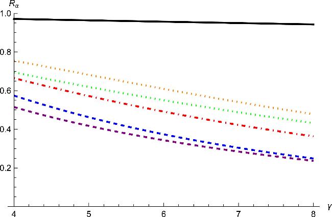
Equation (28) from our results (18) in theorem 1, equation (29) from (12) in [22], equation (30) from [23], equation (31) from [24], equation (32) from [25]. Our result is tighter than the results given in [2225], see figure 1.

Figure 1. The y axis is the lower bound of Rα(ψABC). Solid black line denotes R2(ψABC) for the state given in equation (27). The orange dotted (purple dot dashed, blue dot dashed thick, red dot dashed and green dotted) line represents the lower bound from our result (18) ([2224] and [25]), respectively.
For $\frac{\sqrt{7}-1}{2}\,\leqslant \,\alpha \,\leqslant \,2$, we have the following conclusion.

For any tripartite quantum state ϱABC, we have when $\frac{\sqrt{7}-1}{2}\,\leqslant \,\alpha \lt 2$.

(1) If Rα(ϱAB) ≥ Rα(ϱAC), then

$\begin{eqnarray}\begin{array}{l}{R}_{\alpha }^{\gamma }({\varrho }_{A| BC})\geqslant {R}_{\alpha }^{\gamma }({\varrho }_{A| B})+\lambda {R}_{\alpha }^{\gamma -2}({\varrho }_{A| B}){R}_{\alpha }^{2}({\varrho }_{A| C})\\ +\,({2}^{\lambda }-\lambda -1){R}_{\alpha }^{\gamma }({\varrho }_{A| C}),\end{array}\end{eqnarray}$
for γ ≥ 4.

(2) If Rα(ϱAB) ≤ Rα(ϱAC), then

$\begin{eqnarray}\begin{array}{l}{R}_{\alpha }^{\gamma }({\varrho }_{A| BC})\geqslant {R}_{\alpha }^{\gamma }({\varrho }_{A| C})+\lambda {R}_{\alpha }^{\gamma -2}({\varrho }_{A| C}){R}_{\alpha }^{2}({\varrho }_{A| B})\\ \,+\,({2}^{\lambda }-\lambda -1){R}_{\alpha }^{\gamma }({\varrho }_{A| B}),\end{array}\end{eqnarray}$
for γ ≥ 4, where $\lambda =\frac{\gamma }{2}(\geqslant 2)$.

If Rα(ϱAB) ≥ Rα(ϱAC), we have

$\begin{eqnarray*}\begin{array}{l}{R}_{\alpha }^{\gamma }({\varrho }_{A| BC})\geqslant {[{R}_{\alpha }^{2}({\varrho }_{A| B})+{R}_{\alpha }^{2}({\varrho }_{A| C})]}^{\lambda }\\ =\,{R}_{\alpha }^{\gamma }({\varrho }_{A| B}){\left(1+\frac{{R}_{\alpha }^{2}({\varrho }_{A| C})}{{R}_{\alpha }^{2}({\varrho }_{A| B})}\right)}^{\lambda }\\ \geqslant \,{R}_{\alpha }^{\gamma }({\varrho }_{A| B})+\lambda {R}_{\alpha }^{\gamma -2}({\varrho }_{A| B}){R}_{\alpha }^{2}({\varrho }_{A| C})\\ +\,({2}^{\lambda }-\lambda -1){R}_{\alpha }^{\gamma }({\varrho }_{A| C}),\end{array}\end{eqnarray*}$
where the first inequality is obtained from the inequality (13), the second inequality is derived from the inequality (17) in lemma 2. The inequality (34) can be proves in a similar way.  □

From theorem 4, we get the following theorem for multi-qubit quantum systems. The conditions in theorem 5 reflect the distribution characteristics of entanglement assistance in multipartite systems. The first z (∀ 1 ≤ zN − 3, N ≥ 4) subsystems have sufficiently large squared entanglement values with A, enough to cover the sum of the subsequent subsystems, indicating that these subsystems play a dominant role in the polygamy relations. In contrast, the subsequent subsystems have smaller squared entanglement values, suggesting a more uniform distribution of entanglement resources. This condition allows us to decompose the polygamy inequality into a dominant part and a residual part, thereby obtaining a more precise upper bound.

For any N-qubit quantum state ${\varrho }_{A{B}_{1}\cdots {B}_{N-1}}\in {H}_{A}\otimes {H}_{{B}_{1}}\otimes \cdots \otimes {H}_{{B}_{N-1}}$, if ${R}_{\alpha }^{2}({\varrho }_{A| {B}_{i}})\,\geqslant \displaystyle {\sum }_{l=i+1}^{N-1}{R}_{\alpha }^{2}({\varrho }_{A| {B}_{l}})$ for i = 1, 2, ⋯  , z, and ${R}_{\alpha }^{2}({\varrho }_{A| {B}_{j}})\,\leqslant \,\displaystyle {\sum }_{l=j+1}^{N-1}{R}_{\alpha }^{2}({\varrho }_{A| {B}_{l}})$ for j = z + 1, ⋯  , N − 2, ∀ 1 ≤ z ≤ N − 3 and N ≥ 4, we see that

$\begin{eqnarray}\begin{array}{l}{R}_{\alpha }^{\gamma }({\varrho }_{A| {B}_{1}\cdots {B}_{N-1}})\geqslant \displaystyle \sum _{i=1}^{z}\left\{{({2}^{\lambda }-\lambda -1)}^{i-1}\right.\\ \times \,\left[{R}_{\alpha }^{\gamma }({\varrho }_{A| {B}_{i}})+\lambda {R}_{\alpha }^{\gamma -2}({\varrho }_{A| {B}_{i}})\right.\\ \times \,\left.\left.\left(\displaystyle \sum _{l=i+1}^{N-1}{R}_{\alpha }^{2}({\varrho }_{A| {B}_{l}})\right)\right]\right\}\\ +\,{({2}^{\lambda }-\lambda -1)}^{z}({2}^{\lambda }-1)[{R}_{\alpha }^{\gamma }({\varrho }_{A| {B}_{z+1}})\\ +\,\cdots +{R}_{\alpha }^{\gamma }({\varrho }_{A| {B}_{N-3}})]\\ +\,{({2}^{\lambda }-\lambda -1)}^{z}\left\{({2}^{\lambda }-\lambda -1){R}_{\alpha }^{\gamma }({\varrho }_{A| {B}_{N-2}})\right.\\ +\,\lambda {R}_{\alpha }^{2}({\varrho }_{A| {B}_{N-2}}){R}_{\alpha }^{\gamma -2}({\varrho }_{A| {B}_{N-1}})\\ \left.+\,{R}_{\alpha }^{\gamma }({\varrho }_{A| {B}_{N-1}})\right\},\end{array}\end{eqnarray}$
where γ ≥ 4, $\frac{\sqrt{7}-1}{2}\,\leqslant \,\alpha \lt 2$ and $\lambda =\frac{\gamma }{2}$(≥2).

When ${R}_{\alpha }^{2}({\varrho }_{A| {B}_{i}})\,\geqslant \,\displaystyle {\sum }_{l=i+1}^{N-1}{R}_{\alpha }^{2}({\varrho }_{A| {B}_{l}})$ for i = 1, 2, ⋯ , z, set ${\theta }_{i}^{{\prime} }=\displaystyle {\sum }_{l=i+1}^{N-1}{R}_{\alpha }^{2}({\varrho }_{A| {B}_{l}})/{R}_{\alpha }^{2}({\varrho }_{A| {B}_{i}})$. Substituting ${\theta }_{i}^{{\prime} }$ into the inequality (17) and using inequality (13), we get

$\begin{eqnarray}\begin{array}{l}{R}_{\alpha }^{\gamma }({\varrho }_{A| {B}_{i}\cdots {B}_{N-1}})\geqslant {\left(\displaystyle \sum _{l=i}^{N-1}{R}_{\alpha }^{2}({\varrho }_{A| {B}_{l}})\right)}^{\lambda }\\ \geqslant {R}_{\alpha }^{\gamma }({\varrho }_{A| {B}_{i}})+\lambda {R}_{\alpha }^{\gamma -2}({\varrho }_{A| {B}_{i}})\\ \times \displaystyle \sum _{l=i+1}^{N-1}{R}_{\alpha }^{2}({\varrho }_{A| {B}_{l}})\\ +({2}^{\lambda }-\lambda -1){\left(\displaystyle \sum _{l=i+1}^{N-1}{R}_{\alpha }^{2}({\varrho }_{A| {B}_{l}})\right)}^{\lambda }.\end{array}\end{eqnarray}$
When i = 1, we obtain
$\begin{eqnarray}\begin{array}{l}{R}_{\alpha }^{\gamma }({\varrho }_{A| {B}_{1}\cdots {B}_{N-1}})\\ \geqslant \,{R}_{\alpha }^{\gamma }({\varrho }_{A| {B}_{1}})+\lambda {R}_{\alpha }^{\gamma -2}({\varrho }_{A| {B}_{1}})\left(\displaystyle \sum _{l=2}^{N-1}{R}_{\alpha }^{2}({\varrho }_{A| {B}_{l}})\right)\\ +\,({2}^{\lambda }-\lambda -1){\left(\displaystyle \sum _{l=2}^{N-1}{R}_{\alpha }^{2}({\varrho }_{A| {B}_{l}})\right)}^{\lambda }\\ \geqslant \,{R}_{\alpha }^{\gamma }({\varrho }_{A| {B}_{1}})+\lambda {R}_{\alpha }^{\gamma -2}({\varrho }_{A| {B}_{1}})\left(\displaystyle \sum _{l=2}^{N-1}{R}_{\alpha }^{2}({\varrho }_{A| {B}_{l}})\right)\\ +\,({2}^{\lambda }-\lambda -1){R}_{\alpha }^{\gamma }({\varrho }_{A| {B}_{2}})\\ +\,({2}^{\lambda }-\lambda -1)\lambda {R}_{\alpha }^{\gamma -2}({\varrho }_{A| {B}_{2}})\left(\displaystyle \sum _{l=3}^{N-1}{R}_{\alpha }^{2}({\varrho }_{A| {B}_{l}})\right)\\ +\,{({2}^{\lambda }-\lambda -1)}^{2}{\left(\displaystyle \sum _{l=3}^{N-1}{R}_{\alpha }^{2}({\varrho }_{A| {B}_{l}})\right)}^{\lambda }\\ \geqslant \,\cdots \\ \geqslant \,\displaystyle \sum _{i=1}^{z}\left\{{({2}^{\lambda }-\lambda -1)}^{i-1}\left[{R}_{\alpha }^{\gamma }({\varrho }_{A| {B}_{i}})\right.\right.\\ +\,\left.\left.\lambda {R}_{\alpha }^{\gamma -2}({\varrho }_{A| {B}_{i}})\\ \times \,\left(\displaystyle \sum _{l=i+1}^{N-1}{R}_{\alpha }^{2}({\varrho }_{A| {B}_{l}})\right)\right]\right\}\\ +\,{({2}^{\lambda }-\lambda -1)}^{z}{\left(\displaystyle \sum _{l=z+1}^{N-1}{R}_{\alpha }^{2}({\varrho }_{A| {B}_{l}})\right)}^{\lambda },\end{array}\end{eqnarray}$
by using the inequality (36) iteratively.

When ${R}_{\alpha }^{2}({\varrho }_{A| {B}_{j}})\,\leqslant \,\displaystyle {\sum }_{l=j+1}^{N-1}{R}_{\alpha }^{2}({\varrho }_{A| {B}_{l}})$ for j = z + 1, ⋯ , N − 2, we use a strengthened version of lemma 2. Noting that for 0 ≤ θ ≤ 1 and λ ≥ 2, we have 1 + λθ + (2λ − λ − 1)θλ ≥ 1 + (2λ − 1)θλ. This implies (1 + θ)λ ≥ 1 + (2λ − 1)θλ. Let ${\theta }_{j}^{{\prime} }={R}_{\alpha }^{2}({\varrho }_{A| {B}_{j}})/\displaystyle {\sum }_{l=j+1}^{N-1}{R}_{\alpha }^{2}({\varrho }_{A| {B}_{l}})$. Substituting ${\theta }_{j}^{{\prime} }$ into the above inequality, we obtain

$\begin{eqnarray}\begin{array}{l}{\left(\displaystyle \sum _{l=j}^{N-1}{R}_{\alpha }^{2}({\varrho }_{A| {B}_{l}})\right)}^{\lambda }\geqslant {\left(\displaystyle \sum _{l=j+1}^{N-1}{R}_{\alpha }^{2}({\varrho }_{A| {B}_{l}})\right)}^{\lambda }\\ \,+\,({2}^{\lambda }-1){R}_{\alpha }^{\gamma }({\varrho }_{A| {B}_{j}}).\end{array}\end{eqnarray}$
When j = z + 1, we get
$\begin{eqnarray}\begin{array}{l}{\left(\displaystyle \sum _{l=z+1}^{N-1}{R}_{\alpha }^{2}({\varrho }_{A| {B}_{l}})\right)}^{\lambda }\geqslant {\left(\displaystyle \sum _{l=z+2}^{N-1}{R}_{\alpha }^{2}({\varrho }_{A| {B}_{l}})\right)}^{\lambda }\\ +\,({2}^{\lambda }-1){R}_{\alpha }^{\gamma }({\varrho }_{A| {B}_{z}+1})\\ \geqslant \,{[{R}_{\alpha }^{2}({\varrho }_{A| {B}_{N-2}})+{R}_{\alpha }^{2}({\varrho }_{A| {B}_{N-1}})]}^{\lambda }+({2}^{\lambda }-1)\\ \times \,[{R}_{\alpha }^{\gamma }({\varrho }_{A| {B}_{z+1}})+\cdots +{R}_{\alpha }^{\gamma }({\varrho }_{A| {B}_{N-3}})]\\ \geqslant \,{R}_{\alpha }^{\gamma }({\varrho }_{A| {B}_{N-1}})+\lambda {R}_{\alpha }^{2}({\varrho }_{A| {B}_{N-2}}){R}_{\alpha }^{\gamma -2}({\varrho }_{A| {B}_{N-1}})\\ +\,({2}^{\lambda }-\lambda -1){R}_{\alpha }^{\gamma }({\varrho }_{A| {B}_{N-2}})\\ +\,({2}^{\lambda }-1)[{R}_{\alpha }^{\gamma }({\varrho }_{A| {B}_{z+1}})+\cdots +{R}_{\alpha }^{\gamma }({\varrho }_{A| {B}_{N-3}})],\end{array}\end{eqnarray}$
where the first and second inequalities hold because of the inequality (38), the third inequality is derived from the inequality (17). Combining inequalities (37) and (39), we get the inequality (35).  □

In particular, the following monogamy relations hold.

For any N-qubit quantum state ${\varrho }_{A{B}_{1}\cdots {B}_{N-1}}\in {H}_{A}\otimes {H}_{{B}_{1}}\otimes \cdots \otimes {H}_{{B}_{N-1}}$, if ${R}_{\alpha }^{2}({\varrho }_{A| {B}_{i}})\,\geqslant \,\displaystyle {\sum }_{l=i+1}^{N-1}{R}_{\alpha }^{2}({\varrho }_{A| {B}_{l}})$ for i = 1, 2, ⋯  , N − 2, then

$\begin{eqnarray}\begin{array}{l}{R}_{\alpha }^{\gamma }({\varrho }_{A| {B}_{1}\cdots {B}_{N-1}})\geqslant \displaystyle \sum _{i=1}^{N-2}\left\{{({2}^{\lambda }-\lambda -1)}^{i-1}\right.\\ \left[{R}_{\alpha }^{\gamma }({\varrho }_{A| {B}_{i}})+\lambda {R}_{\alpha }^{\gamma -2}({\varrho }_{A| {B}_{i}})\right.\\ \times \,\left.\left.\left(\displaystyle \sum _{l=i+1}^{N-1}{R}_{\alpha }^{2}({\varrho }_{A| {B}_{l}})\right)\right]\right\}\\ +\,{({2}^{\lambda }-\lambda -1)}^{N-2}{R}_{\alpha }^{\gamma }({\varrho }_{A| {B}_{N}-1}),\end{array}\end{eqnarray}$
where γ ≥ 4, $\frac{\sqrt{7}-1}{2}\,\leqslant \,\alpha \lt 2$ and $\lambda =\frac{\gamma }{2}$(≥2).

Theorems 5 and 6 introduce a new class of monogamy relations in terms of RαE for multi-qubit systems. Similar to the discussions in remark 1, our results in theorems 5 and 6 are better than the ones given in [2427]. Let us consider the example below.

For state (27) given in Example 1, set ${\lambda }_{0}=\frac{\sqrt{5}}{3}$, λ1 = λ4 = 0, ${\lambda }_{2}=\frac{\sqrt{3}}{3}$, ${\lambda }_{3}=\frac{1}{3}$ and $\alpha =\frac{\sqrt{7}-1}{2}$. We have Rα(ψABC) = 0.99265, Rα(ϱAB) = 0.83477 and Rα(ϱAC) = 0.41466. Thus we get

$\begin{eqnarray}\begin{array}{r}{R}_{\alpha }^{\gamma }({\varrho }_{A| B})+({2}^{\frac{\gamma }{2}}-\frac{\gamma }{2}-1){R}_{\alpha }^{\gamma }({\varrho }_{A| C})\\ +\frac{\gamma }{2}{R}_{\alpha }^{\gamma -2}({\varrho }_{A| B}){R}_{\alpha }({\varrho }_{A| C})\\ =\,{(0.83477)}^{\gamma }+\frac{\gamma }{2}{(0.41466)}^{2}{(0.83477)}^{\gamma -2}\\ +({2}^{\frac{\gamma }{2}}-\frac{\gamma }{2}-1){(0.41466)}^{\gamma },\end{array}\end{eqnarray}$
$\begin{eqnarray}\begin{array}{r}{R}_{\alpha }^{\gamma }({\varrho }_{A| B})+{R}_{\alpha }^{\gamma }({\varrho }_{A| C})={(0.83477)}^{\gamma }+{(0.41466)}^{\gamma },\end{array}\end{eqnarray}$
$\begin{eqnarray}\begin{array}{r}{R}_{\alpha }^{\gamma }({\varrho }_{A| B})+({2}^{\gamma }-1){R}_{\alpha }^{\gamma }({\varrho }_{A| C})\\ =\,{(0.83477)}^{\gamma }+({2}^{\gamma }-1){(0.41466)}^{\gamma },\end{array}\end{eqnarray}$
$\begin{eqnarray}\begin{array}{r}{R}_{\alpha }^{\gamma }({\varrho }_{A| B})+\frac{\gamma }{4}{R}_{\alpha }^{\gamma -2}({\varrho }_{A| B}){R}_{\alpha }({\varrho }_{A| C})\\ +\,({2}^{\frac{\gamma }{2}}-\frac{\gamma }{4}-1){R}_{\alpha }^{\gamma }({\varrho }_{A| C})\\ =\,{(0.83477)}^{\gamma }+\frac{\gamma }{4}{(0.41466)}^{2}{(0.83477)}^{\gamma -2}\\ +\,({2}^{\frac{\gamma }{2}}-\frac{\gamma }{4}-1){(0.41466)}^{\gamma },\end{array}\end{eqnarray}$
$\begin{eqnarray}\begin{array}{r}{R}_{\alpha }^{\gamma }({\varrho }_{A| B})+\frac{{\gamma }^{2}}{2(\gamma +2)}{R}_{\alpha }^{\gamma -2}({\varrho }_{A| B}){R}_{\alpha }({\varrho }_{A| C})\\ +\,({2}^{\frac{\gamma }{2}}-\frac{{\gamma }^{2}}{2(\gamma +2)}-1){R}_{\alpha }^{\gamma }({\varrho }_{A| C})\\ =\,{(0.83477)}^{\gamma }+\frac{{\gamma }^{2}}{2(\gamma +2)}{(0.41466)}^{2}{(0.83477)}^{\gamma -2}\\ +\,({2}^{\frac{\gamma }{2}}-\frac{{\gamma }^{2}}{2(\gamma +2)}-1){(0.41466)}^{\gamma }.\end{array}\end{eqnarray}$
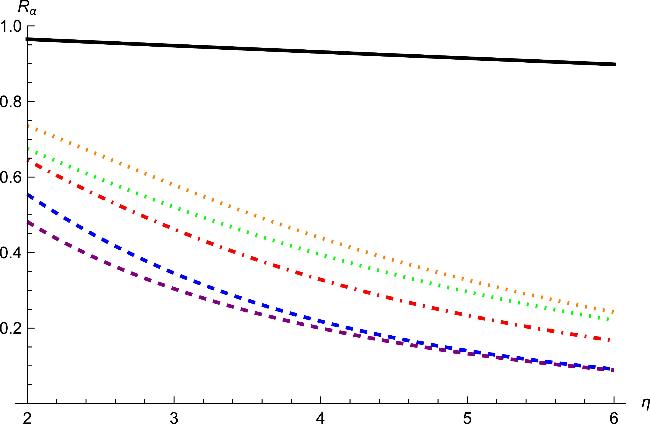
Equation (41) from our result (33) in theorem 4, equation (42) from (13) in [26], equation (43) from [27], equation (44) from [24] and equation (45) from [25], one sees that our result is better than the results given in [2427], see figure 2.

Figure 2. The y axis is the lower bound of Rα(ψABC). Solid black line denotes Rα(ψABC) of the state (27). The orange dotted (purple dot dashed, blue dot dashed thick, red dot dashed and green dotted) line represents the lower bound from our result (33) ([24, 26, 27] and [25]), respectively.

4. Tighter polygamy relations for RαEoA

In this section, we study the polygamy relations of RαEoA with $\frac{\sqrt{7}-1}{2}\,\leqslant \,\alpha \,\leqslant \,\frac{\sqrt{13}-1}{2}$ for N-qubit systems. In [23], the relation (15) has been further improved to be
$\begin{eqnarray}\begin{array}{r}{[{R}_{\alpha }^{a}({\varrho }_{A| {B}_{1}\cdots {B}_{N-1}})]}^{t}\leqslant {[{R}_{\alpha }^{a}({\varrho }_{A| {B}_{1}})]}^{t}\\ +\,({2}^{t}-1){[{R}_{\alpha }^{a}({\varrho }_{A| {B}_{2}})]}^{t}+\cdots \\ \,+\,{({2}^{t}-1)}^{z-1}{[{R}_{\alpha }^{a}({\varrho }_{A| {B}_{z}})]}^{t}\\ \,+\,{({2}^{t}-1)}^{z+1}\left({[{R}_{\alpha }^{a}({\varrho }_{A| {B}_{z+1}})]}^{t}\right.\\ \,\left.+\cdots +{[{R}_{\alpha }^{a}({\varrho }_{A| {B}_{N-2}})]}^{t}\right)\\ \,+\,{({2}^{t}-1)}^{z}{[{R}_{\alpha }^{a}({\varrho }_{A| {B}_{N-1}})]}^{t},\end{array}\end{eqnarray}$
for 0 ≤ t ≤ 1, where ${R}_{\alpha }^{a}({\varrho }_{A{B}_{i}})\,\geqslant \,{R}_{\alpha }^{a}({\varrho }_{A| {B}_{i+1}\cdots {B}_{N-1}})$ for i = 1, 2, ⋯  , z, and ${R}_{\alpha }^{a}({\varrho }_{A{B}_{j}})\,\leqslant \,{R}_{\alpha }^{a}({\varrho }_{A| {B}_{j+1}\cdots {B}_{N-1}})$ for j = z + 1, ⋯  , N − 2, ∀1 ≤ zN − 3, N ≥ 4 and $\frac{\sqrt{7}-1}{2}\,\leqslant \,\alpha \,\leqslant \,\frac{\sqrt{13}-1}{2}$.
Next, we illustrate that the above polygamy relations can be tightened under some conditions. We first propose the following lemma.

For any 0 ≤ θ ≤ 1 and 0 ≤ v ≤ 1, then

$\begin{eqnarray}\begin{array}{l}{(1+\theta )}^{v}\leqslant 1+{2}^{v-2}v\theta +({2}^{v}-{2}^{v-2}v-1){\theta }^{v}\\ \leqslant 1+({2}^{v}-1){\theta }^{v}.\end{array}\end{eqnarray}$

If θ = 0, the inequality holds. If θ ≠ 0, the core idea is to reformulate the desired inequality. Observing that equation (47) is equivalent to $\frac{{(1+\theta )}^{v}-{2}^{v-2}v\theta -1}{{\theta }^{v}}\,\geqslant \,{2}^{v}-{2}^{v-2}v-1$, we consider the function $f(\theta ,v)\,=\frac{{(1+\theta )}^{v}-{2}^{v-2}v\theta -1}{{\theta }^{v}}$ for 0 ≤ θ ≤ 1 and 0 ≤ v ≤ 1. Proving the inequality (47) is now equivalent to showing f(θv) ≤ f(1, v) = 2v − 2v−2v − 1. To establish this, we examine the monotonicity of f with respect to θ. We have

$\begin{eqnarray*}\begin{array}{l}\frac{\partial f(\theta ,v)}{\partial \theta }=\frac{[v{(1+\theta )}^{v-1}-{2}^{v-2}v]{\theta }^{v}-\left[{(1+\theta )}^{v}-{2}^{v-2}v\theta -1\right]v{\theta }^{v-1}}{{\theta }^{2v}}\\ =\,\frac{v{\theta }^{v-1}[1+{2}^{v-2}\theta (v-1)-{(1+\theta )}^{v-1}]}{{\theta }^{2v}}.\end{array}\end{eqnarray*}$
Let g(θv) = (1 + θ)v−1 − 1 − 2v−2θ(v − 1). Then $\frac{\partial g(\theta ,v)}{\partial \theta }=(v-1)[{(1+\theta )}^{v-2}-{2}^{v-2}]\,\leqslant \,0$ for 0 ≤ θ ≤ 1 and 0 ≤ v ≤ 1. Hence, g(θv) is a decreasing function of θ for fixed v, and g(θv) ≤ g(0, v) = 0. Thus, $\frac{\partial f(\theta ,v)}{\partial \theta }\,\geqslant \,0$. f(θv) is an increasing function of θ, i.e., f(θv) ≤ f(1, v) = 2v − 2v−2v − 1. Then, we have (1 + θ)v ≤ 1 + 2v−2 + (2v − 2v−2v − 1)θv. Since 2v−2v(θ − θv) ≤ 0 for 0 ≤ θ ≤ 1 and 0 ≤ v ≤ 1, we get 2v−2 + (2v − 2v−2v − 1)θv ≤ 1 + (2v − 1)θv.  □

By using lemma 3, we have the following polygamy relations which is tighter than the relations (15) and (46) in references [28] and [23].

For any tripartite quantum state ϱABC, if ${R}_{\alpha }^{a}({\varrho }_{A| B})\,\geqslant \,{R}_{\alpha }^{a}({\varrho }_{A| C})$, we see that

$\begin{eqnarray}\begin{array}{l}{({R}_{\alpha }^{a})}^{t}({\varrho }_{A| BC})\leqslant {({R}_{\alpha }^{a})}^{t}({\varrho }_{A| B})+h{({R}_{\alpha }^{a})}^{t}({\varrho }_{A| C})\\ \quad +\,{2}^{t-2}t[{R}_{\alpha }^{a}({\varrho }_{A| C}){({R}_{\alpha }^{a})}^{t-1}({\varrho }_{A| B})\\ \quad -\,{({R}_{\alpha }^{a})}^{t}({\varrho }_{A| C})],\end{array}\end{eqnarray}$
for 0 ≤ t ≤ 1, where h = 2t − 1.

It has been shown that ${R}_{\alpha }^{a}({\varrho }_{A| BC})\,\leqslant \,{R}_{\alpha }^{a}({\varrho }_{A| B})\,+{R}_{\alpha }^{a}({\varrho }_{A| C})$ in (15). In terms of ${R}_{\alpha }^{a}({\varrho }_{A| B})\,\geqslant \,{R}_{\alpha }^{a}({\varrho }_{A| C})$ we have

$\begin{eqnarray}\begin{array}{l}{({R}_{\alpha }^{a})}^{t}({\varrho }_{A| BC})\leqslant {[{R}_{\alpha }^{a}({\varrho }_{A| B})+{R}_{\alpha }^{a}({\varrho }_{A| C})]}^{t}\\ \quad =\,{({R}_{\alpha }^{a})}^{t}({\varrho }_{A| B}){\left(1+\frac{{R}_{\alpha }^{a}({\varrho }_{A| C})}{{R}_{\alpha }^{a}({\varrho }_{A| B})}\right)}^{t}\\ \quad \leqslant \,{({R}_{\alpha }^{a})}^{t}({\varrho }_{A| B})\left[1+{2}^{t-2}t\frac{{R}_{\alpha }^{a}({\varrho }_{A| C})}{{R}_{\alpha }^{a}({\varrho }_{A| B})}\right.\\ \quad \left.+\,({2}^{t}-{2}^{t-2}t-1)\frac{{({R}_{\alpha }^{a})}^{t}({\varrho }_{A| C})}{{({R}_{\alpha }^{a})}^{t}({\varrho }_{A| B})}\right]\\ \quad =\,{({R}_{\alpha }^{a})}^{t}({\varrho }_{A| B})+h{({R}_{\alpha }^{a})}^{t}({\varrho }_{A| C})\\ \quad +\,{2}^{t-2}t[{R}_{\alpha }^{a}({\varrho }_{A| C}){({R}_{\alpha }^{a})}^{t-1}({\varrho }_{A| B})\\ \quad -\,{({R}_{\alpha }^{a})}^{t}({\varrho }_{A| C})],\end{array}\end{eqnarray}$
where the second inequality is due to lemma 3.  □

From lemma 3, we have

$\begin{eqnarray*}\begin{array}{l}{(1+\theta )}^{v}\leqslant 1+{2}^{v-2}v\theta +({2}^{v}-{2}^{v-2}v-1){\theta }^{v}\\ \leqslant 1+({2}^{v}-1){\theta }^{v}\quad (\,\rm{The inequality in [25]}\,).\end{array}\end{eqnarray*}$
Since θ − θλ ≤ 0 for 0 ≤ θ ≤ 1 and 0 ≤ v ≤ 1, obviously our inequality given in theorem 7 is tighter than the ones presented in [23, 28].

The following theorem gives tighter upper bounds of ${({R}_{\alpha }^{a})}^{t}({\varrho }_{A| {B}_{1}\cdots {B}_{N-1}})$ for 0 ≤ t ≤ 1.

For any N-qubit mixed state ${\varrho }_{A{B}_{1}\cdots {B}_{N-1}}\in {H}_{A}\otimes {H}_{{B}_{1}}\otimes \cdots \otimes {H}_{{B}_{N-1}}$, if ${R}_{\alpha }^{a}({\varrho }_{A| {B}_{i}})\,\geqslant \,\displaystyle {\sum }_{k=i+1}^{N-1}{R}_{\alpha }^{a}({\varrho }_{A| {B}_{k}})$ for i = 1, 2, ⋯  , N − 2, we obtain

$\begin{eqnarray}\begin{array}{rcl}{({R}_{\alpha }^{a})}^{t}({\varrho }_{A| {B}_{1}\cdots {B}_{N-1}}) & \leqslant & \displaystyle \sum _{i=1}^{N-2}{h}^{i-1}[{({R}_{\alpha }^{a})}^{t}({\varrho }_{A| {B}_{i}})+{N}_{A{B}_{i}}]\\ & & +{h}^{N-2}{({R}_{\alpha }^{a})}^{t}({\varrho }_{A| {B}_{N-1}}),\end{array}\end{eqnarray}$
for 0 ≤ t ≤ 1, where h = 2t − 1 and ${N}_{A{B}_{i}}$ = ${2}^{t-2}t\left(\displaystyle {\sum }_{k=i+1}^{N-1}{R}_{\alpha }({\varrho }_{A| {B}_{k}})\right.$ ${({R}_{\alpha }^{a})}^{t-1}({\varrho }_{A| {B}_{i}})$ $-\left.{[\displaystyle {\sum }_{k=i+1}^{N-1}{R}_{\alpha }({\varrho }_{A| {B}_{k}})]}^{t}\right)$.

According to (15), we get

$\begin{eqnarray}\begin{array}{l}{({R}_{\alpha }^{a})}^{t}({\varrho }_{A| {B}_{1}\cdots {B}_{N-1}})\leqslant [{R}_{\alpha }^{a}({\varrho }_{A| {B}_{1}})\\ +\,{R}_{\alpha }^{a}({\varrho }_{A| {B}_{2}})+\cdots +{R}_{\alpha }^{a}({\varrho }_{A| {B}_{N-1}}){]}^{t}\\ \leqslant \,{({R}_{\alpha }^{a})}^{t}({\varrho }_{A| {B}_{1}})+h{\left[\displaystyle \sum _{k=2}^{N-1}{R}_{\alpha }^{a}({\varrho }_{A| {B}_{k}})\right]}^{t}+{2}^{t-2}t\left(\displaystyle \sum _{k=2}^{N-1}{R}_{\alpha }^{a}({\varrho }_{A| {B}_{k}})\right.\\ \times \left.{({R}_{\alpha }^{a})}^{t-1}({\varrho }_{A| {B}_{1}})-{\left[\displaystyle \sum _{k=2}^{N-1}{R}_{\alpha }^{a}({\varrho }_{A| {B}_{k}})\right]}^{t}\right)\\ \leqslant \,{({R}_{\alpha }^{a})}^{t}({\varrho }_{A| {B}_{1}})+h\left[{({R}_{\alpha }^{a})}^{t}({\varrho }_{A| {B}_{2}})+h{\left[\displaystyle \sum _{k=3}^{N-1}{R}_{\alpha }^{a}({\varrho }_{A| {B}_{k}})\right]}^{t}\right.\\ +\,{2}^{t-2}t\left(\displaystyle \sum _{k=3}^{N-1}{R}_{\alpha }^{a}({\varrho }_{A| {B}_{k}})\right.\\ \times \,\left.\left.{({R}_{\alpha }^{a})}^{t-1}({\varrho }_{A| {B}_{2}})-{\left[\displaystyle \sum _{k=3}^{N-1}{R}_{\alpha }^{a}({\varrho }_{A| {B}_{k}})\right]}^{t}\right)\right]\\ +\,{2}^{t-2}t\left(\displaystyle \sum _{k=2}^{N-1}{R}_{\alpha }^{a}({\varrho }_{A| {B}_{k}})\right.\\ \times \,\left.{({R}_{\alpha }^{a})}^{t-1}({\varrho }_{A| {B}_{1}})-{\left[\displaystyle \sum _{k=2}^{N-1}{R}_{\alpha }^{a}({\varrho }_{A| {B}_{k}})\right]}^{t}\right)\\ \leqslant \,\cdots \\ \leqslant \,{({R}_{\alpha }^{a})}^{t}({\varrho }_{A| {B}_{1}})+h{({R}_{\alpha }^{a})}^{t}({\varrho }_{A| {B}_{2}})+\cdots +{h}^{N-2}{({R}_{\alpha }^{a})}^{t}({\varrho }_{A| {B}_{N-1}})\\ +\,{h}^{N-3}{2}^{t-2}t\left({R}_{\alpha }^{a}({\varrho }_{A| {B}_{N-1}})\right.\\ \times \,\left.{({R}_{\alpha }^{a})}^{t-1}({\varrho }_{A| {B}_{N-2}})-{({R}_{\alpha }^{a})}^{t}({\varrho }_{A| {B}_{N-1}})\right)\\ +\,\cdots \\ +\,h{2}^{t-2}t\left(\displaystyle \sum _{k=3}^{N-1}{R}_{\alpha }^{a}({\varrho }_{A| {B}_{k}})\right.\\ \times \,\left.{({R}_{\alpha }^{a})}^{t-1}({\varrho }_{A| {B}_{2}})-{\left[\displaystyle \sum _{k=3}^{N-1}{R}_{\alpha }^{a}({\varrho }_{A| {B}_{k}})\right]}^{t}\right)\\ +\,{2}^{t-2}t\left(\displaystyle \sum _{k=2}^{N-1}{R}_{\alpha }^{a}({\varrho }_{A| {B}_{k}})\right.\\ \times \,\left.{({R}_{\alpha }^{a})}^{t-1}({\varrho }_{A| {B}_{1}})-{\left[\displaystyle \sum _{k=2}^{N-1}{R}_{\alpha }^{a}({\varrho }_{A| {B}_{k}})\right]}^{t}\right),\end{array}\end{eqnarray}$
where the second inequality is due to lemma 3. By the denotation of ${N}_{A{B}_{i}}$, we complete the proof.  □

Typically, the conditions for inequalities (15) are not fulfilled in every case. As a consequence, we propose a general polygamy inequality.

For any N-qubit mixed state ${\varrho }_{A{B}_{1}\cdots {B}_{N-1}}\in {H}_{A}\otimes {H}_{{B}_{1}}\otimes \cdots \otimes {H}_{{B}_{N-1}}$, if ${R}_{\alpha }^{a}({\varrho }_{A| {B}_{i}})\,\geqslant \,\displaystyle {\sum }_{k=i+1}^{N-1}{R}_{\alpha }^{a}({\varrho }_{A| {B}_{k}})$ for i = 1, 2, ⋯  , z, and ${R}_{\alpha }^{a}({\varrho }_{A| {B}_{j}})\,\leqslant \,\displaystyle {\sum }_{k=j+1}^{N-1}{R}_{\alpha }^{a}({\varrho }_{A| {B}_{k}})$ for j = z + 1, ⋯  , N − 2, ∀ 1 ≤ zN − 3 and N ≥ 4, then

$\begin{eqnarray}\begin{array}{l}{({R}_{\alpha }^{a})}^{t}({\varrho }_{A| {B}_{1}\cdots {B}_{N-1}})\\ \leqslant \,\displaystyle \sum _{i=1}^{z}{h}^{i-1}[{({R}_{\alpha }^{a})}^{t}({\varrho }_{A| {B}_{i}})+{N}_{A{B}_{i}}]\\ +\,{h}^{z}\displaystyle \sum _{j=z+1}^{N-2}[h{({R}_{\alpha }^{a})}^{t}({\varrho }_{A| {B}_{j}})+{\overline{N}}_{A{B}_{j}}]\\ +\,{h}^{z}{({R}_{\alpha }^{a})}^{t}({\varrho }_{A| {B}_{N-1}}),\end{array}\end{eqnarray}$
for 0 ≤ t ≤ 1, where h = 2t − 1, ${N}_{A{B}_{i}}$ = ${2}^{t-2}t\left(\displaystyle {\sum }_{k=i+1}^{N-1}{R}_{\alpha }^{a}({\varrho }_{A| {B}_{k}})\right.$ $\times {({R}_{\alpha }^{a})}^{t-1}({\varrho }_{A| {B}_{i}})$ $-\left.{[\displaystyle {\sum }_{k=i+1}^{N-1}{R}_{\alpha }^{a}({\varrho }_{A| {B}_{k}})]}^{t}\right)$ and ${\overline{N}}_{A{B}_{j}}$ = ${2}^{t-2}t\left({R}_{\alpha }^{a}({\varrho }_{A| {B}_{j}})\right.$ ${[\displaystyle {\sum }_{k=j+1}^{N-1}{R}_{\alpha }^{a}({\varrho }_{A| {B}_{k}})]}^{t-1}$ $-\left.{({R}_{\alpha }^{a})}^{t}({\varrho }_{A| {B}_{j}})\right)$.

From the proof of theorem 8, we see that

$\begin{eqnarray}\begin{array}{l}{({R}_{\alpha }^{a})}^{t}({\varrho }_{A| {B}_{1}\cdots {B}_{N-1}})\leqslant \displaystyle \sum _{i=1}^{z}{h}^{i-1}[{({R}_{\alpha }^{a})}^{t}({\varrho }_{A| {B}_{i}})+{N}_{A{B}_{i}}]\\ \,+\,{h}^{z}{\left[\displaystyle \sum _{k=z+1}^{N-1}{R}_{\alpha }^{a}({\varrho }_{A| {B}_{k}})\right]}^{t}.\end{array}\end{eqnarray}$

In addition, since ${R}_{\alpha }^{a}({\varrho }_{A| {B}_{j}})\,\leqslant \,\displaystyle \sum _{k=j+1}^{N-1}{R}_{\alpha }^{a}({\varrho }_{A| {B}_{k}})$ for j = z + 1, ⋯  , N − 2, we obtain

$\begin{eqnarray}\begin{array}{l}{\left[\displaystyle \sum _{k=z+1}^{N-1}{R}_{\alpha }^{a}({\varrho }_{A| {B}_{k}})\right]}^{t}\\ \leqslant {\left[\displaystyle \sum _{k=z+2}^{N-1}{R}_{\alpha }^{a}({\varrho }_{A| {B}_{k}})\right]}^{t}+h{({R}_{\alpha }^{a})}^{t}({\varrho }_{A| {B}_{z+1}})\\ +{2}^{t-2}t\left({R}_{\alpha }^{a}({\varrho }_{A| {B}_{z+1}})\right.\\ \times \,\left.{\left[\displaystyle \sum _{k=z+2}^{N-1}{R}_{\alpha }^{a}({\varrho }_{A| {B}_{k}})\right]}^{t-1}-{({R}_{\alpha }^{a})}^{t}({\varrho }_{A| {B}_{z+1}})\right)\\ \leqslant \cdots \\ \leqslant \displaystyle \sum _{j=z+1}^{N-2}[h{({R}_{\alpha }^{a})}^{t}({\varrho }_{A| {B}_{j}})+{\overline{N}}_{A{B}_{j}}]\\ +{({R}_{\alpha }^{a})}^{t}({\varrho }_{A| {B}_{N-1}}).\end{array}\end{eqnarray}$

By the denotations of ${N}_{A{B}_{j}}$ and ${\overline{N}}_{A{B}_{j}}$, from the inequalities (53) and (54) we complete the proof.  □

Consider the following example to demonstrate the tightness of our polygamy relations of multi-qubit entanglement.

Consider a three-qubit generalised W-class state,

$\begin{eqnarray}| \psi {\rangle }_{A| BC}=\frac{1}{\sqrt{6}}| 100\rangle +\frac{1}{\sqrt{6}}| 010\rangle +\frac{2}{\sqrt{6}}| 001\rangle .\end{eqnarray}$
We get ${R}_{\frac{\sqrt{7}-1}{2}}({\psi }_{A| BC})=0.698944$, ${R}_{\frac{\sqrt{7}-1}{2}}({\varrho }_{A| B})\,=0.241379$ and ${R}_{\frac{\sqrt{7}-1}{2}}({\varrho }_{A| C})=0.607261$. Thus one gets
$\begin{eqnarray}\begin{array}{r}{[{R}_{\alpha }^{a}]}^{t}({\varrho }_{A| B})+({2}^{t}-{2}^{t-2}t-1){[{R}_{\alpha }^{a}]}^{t}({\varrho }_{A| C})\\ +\,{2}^{t-2}t{[{R}_{\alpha }^{a}]}^{t-1}({\varrho }_{A| B}){R}_{\alpha }^{a}({\varrho }_{A| C})\\ =\,{(0.241379)}^{t}+({2}^{t}-{2}^{t-2}t-1){(0.607261)}^{t}\\ +\,{2}^{t-2}t{(0.241379)}^{t-1}(0.607261),\end{array}\end{eqnarray}$
$\begin{eqnarray}\begin{array}{r}{[{R}_{\alpha }^{a}]}^{t}({\varrho }_{AB})+{[{R}_{\alpha }^{a}]}^{t}({\varrho }_{AC})\\ =\,{(0.241379)}^{t}+{(0.607261)}^{t},\end{array}\end{eqnarray}$
$\begin{eqnarray}\begin{array}{r}{[{R}_{\alpha }^{a}]}^{t}({\varrho }_{AB})+({2}^{t}-1){[{R}_{\alpha }^{a}]}^{t}({\varrho }_{AC})\\ =\,{(0.241379)}^{t}+({2}^{t}-1){(0.607261)}^{t}.\end{array}\end{eqnarray}$

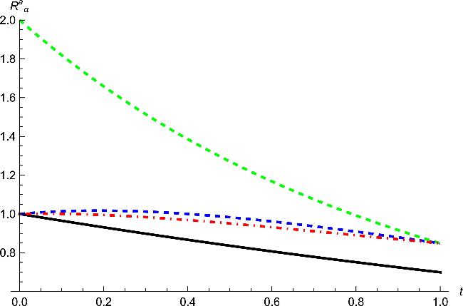
Equation (56) from our result (48) in theorem 7, equation (57) from (15) in [28], equation (58) from (46) in [23]. Our findings are observed to be tighter than the results given in [28] and [23], respectively, see figure 3.

Figure 3. The y axis is the upper bound of ${R}_{\alpha }^{a}({\psi }_{A| BC})$. Solid black line denotes ${R}_{\alpha }^{a}({\psi }_{A| BC})$ for the state (55). The red dot dashed (green dotted, blue dot dashed thick) line represents the upper bound from our result (48) ((15) in [28], (46) in [23]).

5. Residual entanglement of RαE

For a 2 ⨂ 2 ⨂ d quantum pure state ∣ψABC, the three tangle is expressed as [40],
$\begin{eqnarray}\tau (| \psi {\rangle }_{ABC})={{\mathscr{C}}}^{2}(| \psi {\rangle }_{A| BC})-{{\mathscr{C}}}^{2}({\varrho }_{A| B})-{{\mathscr{C}}}^{2}({\varrho }_{A| C}),\end{eqnarray}$
where ${\varrho }_{AB(AC)}={{\rm{Tr}}}_{C(B)}(| \psi {\rangle }_{ABC}\langle \psi | )$. Additionally, the three-tangle can also be characterized by the concurrence of assistance, an important entanglement measure that quantifies the maximum average concurrence shared by two parties with the assistance of the third party [40]:
$\begin{eqnarray}{{\mathscr{C}}}_{a}^{2}({\varrho }_{A| B})={{\mathscr{C}}}^{2}({\varrho }_{A| B})+\tau (| \psi {\rangle }_{ABC}).\end{eqnarray}$
For a mixed state ϱABC, the three tangle is expressed as
$\begin{eqnarray}\tau ({\varrho }_{ABC})=\min \displaystyle \sum _{i}{p}_{i}\sqrt{\tau (| {\psi }^{i}{\rangle }_{ABC})},\end{eqnarray}$
where the minimum is taken over all possible pure state decompositions {pi, ∣ψiAB} of ϱABC.
Similar to the three tangle determined by concurrence, for the three-qubit state ∣ψABC ∈ HA ⨂ HB ⨂ HC, we define the residual entanglement given by the μth (μ ≥ 1) power of RαE by using the relation (12),
$\begin{eqnarray}{\tau }_{\mu }^{R}(| \psi {\rangle }_{ABC})={R}_{\alpha }^{\mu }(| \psi {\rangle }_{A| BC})-{R}_{\alpha }^{\mu }({\varrho }_{A| B})-{R}_{\alpha }^{\mu }({\varrho }_{A| C}),\end{eqnarray}$
where α ≥ 2. We have the following relations among the residual entanglement of RαE, RαEoA and three tangle.

For a three-qubit pure state ∣ψABC, we see that

$\begin{eqnarray}{\tau }_{\mu }^{R}(| \psi {\rangle }_{ABC})\geqslant {f}_{\alpha }^{\mu }\left(\sqrt{\tau (| \psi {\rangle }_{ABC}})\right),\end{eqnarray}$
and
$\begin{eqnarray}{({R}_{\alpha }^{a})}^{\mu }({\varrho }_{A| B})\geqslant {R}_{\alpha }^{\mu }({\varrho }_{A| B})+{f}_{\alpha }^{\mu }\left(\sqrt{\tau (| \psi {\rangle }_{ABC}})\right),\end{eqnarray}$
where α ≥ 2, μ ≥ 1, fα is given in (9), ${\varrho }_{AB}={{\rm{Tr}}}_{C}(| \psi {\rangle }_{ABC}\langle \psi | )$ and τ(∣ψABC) is the three tangle of concurrence.

For α ≥ 2 and μ ≥ 1 we get

$\begin{eqnarray}\begin{array}{rcl}{f}_{\alpha }^{\mu }(\sqrt{{\xi }_{1}^{2}+{\xi }_{2}^{2}}) & = & {({f}_{\alpha }(\sqrt{{\xi }_{1}^{2}+{\xi }_{2}^{2}}))}^{\mu }\\ & \geqslant & {({f}_{\alpha }({\xi }_{1})+{f}_{\alpha }({\xi }_{2}))}^{\mu }\\ & \geqslant & {f}_{\alpha }^{\mu }({\xi }_{1})+{f}_{\alpha }^{\mu }({\xi }_{2}),\end{array}\end{eqnarray}$
where the first inequality is due to the inequality (10), and the second inequality is derived from the inequality (1 + r)s ≥ 1 + rs for r ≥ 0 and s ≥ 1.

Based on the definition of ${\tau }_{\mu }^{R}(| \psi {\rangle }_{ABC})$, we have

$\begin{eqnarray*}\begin{array}{l}{\tau }_{\mu }^{R}(| \psi {\rangle }_{ABC})={R}_{\alpha }^{\mu }(| \psi {\rangle }_{A| BC})-{R}_{\alpha }^{\mu }({\varrho }_{A| B})-{R}_{\alpha }^{\mu }({\varrho }_{A| C})\\ \,=\,{f}_{\alpha }^{\mu }({\mathscr{C}}(| \psi {\rangle }_{A| BC}))-{f}_{\alpha }^{\mu }({\mathscr{C}}({\varrho }_{A| B}))-{f}_{\alpha }^{\mu }({\mathscr{C}}({\varrho }_{A| C}))\\ \,=\,{f}_{\alpha }^{\mu }\left(\sqrt{{{\mathscr{C}}}^{2}({\varrho }_{A| B})+{{\mathscr{C}}}^{2}({\varrho }_{A| C})+\tau (| \psi {\rangle }_{A| BC})}\right)\\ \quad -\,{f}_{\alpha }^{\mu }({\mathscr{C}}({\varrho }_{A| B}))-{f}_{\alpha }^{\mu }({\mathscr{C}}({\varrho }_{A| C}))\\ \,\geqslant \,{f}_{\alpha }^{\mu }\left(\sqrt{\tau (| \psi {\rangle }_{ABC}})\right),\end{array}\end{eqnarray*}$
where the third equality is obtained from the equation (59), and we have used (65) to get the last inequality.

According to equation (60), we have

$\begin{eqnarray*}\begin{array}{l}\,{({R}_{\alpha }^{a})}^{\mu }({\varrho }_{A| B})\,\geqslant \,{f}_{\alpha }^{\mu }({{\mathscr{C}}}_{a}({\varrho }_{A| B}))\\ \,=\,{f}_{\alpha }^{\mu }(\sqrt{{{\mathscr{C}}}^{2}({\varrho }_{A| B})+\tau (| \psi {\rangle }_{ABC})})\\ \,\geqslant \,{f}_{\alpha }^{\mu }({\mathscr{C}}({\varrho }_{A| B}))+{f}_{\alpha }^{\mu }\left(\sqrt{\tau (| \psi {\rangle }_{ABC}})\right)\\ \,=\,{R}_{\alpha }^{\mu }({\varrho }_{A| B})+{f}_{\alpha }^{\mu }\left(\sqrt{\tau (| \psi {\rangle }_{ABC}})\right),\end{array}\end{eqnarray*}$
where the first inequality is obtained from the relation ${R}_{\alpha }^{a}({\varrho }_{AB})\,\geqslant \,{f}_{\alpha }({{\mathscr{C}}}_{a}({\varrho }_{AB}))$ with $\alpha \,\geqslant \,\frac{\sqrt{7}-1}{2}$ in [28], the second inequality is derived from the inequality (65), and we have used the equality (8) to obtain the last equality.  □

The relations among RαE, RαEoA and the three tangle given in theorem 10 can be utilized to derive a lower bound of RαEoA. Let us consider the following example.

For the superpositions of the Greenberger–Horne–Zeilinger-state and the W-state,
$\begin{eqnarray}\begin{array}{r}| {\rm{\Psi }}{\rangle }_{ABC}=\sqrt{\frac{1}{2}}| {\rm{G}}{\rm{H}}{\rm{Z}}\rangle -\sqrt{\frac{1}{2}}| W\rangle ,\end{array}\end{eqnarray}$
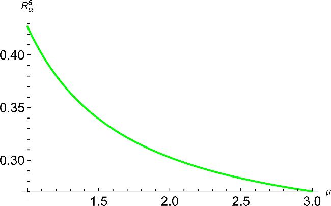
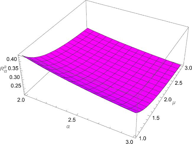
where $| {\rm{G}}{\rm{H}}{\rm{Z}}\rangle =\frac{1}{\sqrt{2}}(| 000\rangle +| 111\rangle )$ and $| W\rangle =\frac{1}{\sqrt{3}}(| 100\rangle \,+| 010\rangle +| 001\rangle )$, according to theorem 10 we get the lower bound of ${R}_{\alpha }^{a}({\varrho }_{A| B})$, ${R}_{\alpha }^{a}({\varrho }_{A| B})\,\geqslant \,{({R}_{\alpha }^{\mu }({\varrho }_{A| B})+{f}_{\alpha }^{\mu }(\sqrt{\tau (| \psi {\rangle }_{ABC})}))}^{\frac{1}{\mu }}$, where ${\varrho }_{AB}={{\rm{Tr}}}_{C}(| {\rm{\Psi }}{\rangle }_{ABC}\langle {\rm{\Psi }}| )$, see figures 4 and 5. When α =2, one gets the optimal lower bound 0.4269 of ${R}_{\alpha }^{a}({\varrho }_{AB})$ at μ = 1.

Figure 4. The purple surface represents the lower bound of ${R}_{\alpha }^{a}({\varrho }_{AB})$ for the state (66) with α ≥ 2 and μ ≥ 1.
Figure 5. The green line represents the lower bound of ${R}_{\alpha }^{a}({\varrho }_{AB})$ for the state (66) with α = 2 and μ ≥ 1.

6. Conclusion

Entanglement monogamy and polygamy relations are two intrinsic characteristics of multipartite entangled states. Our results refine the characterization of multi-qubit entanglement shareability and distribution through RαE. We have provided classes of tighter monogamy relations in terms of the η-th (η ≥ 2) power of RαE for α ≥ 2, and the γ-th (γ ≥ 4) power of RαE for $\frac{\sqrt{7-1}}{2}\,\leqslant \,\alpha \lt 2$, respectively. Moreover, we have presented polygamy relations satisfied by the tth power of RαEoA with $\frac{\sqrt{7}-1}{2}\,\leqslant \,\alpha \lt \frac{\sqrt{13}-1}{2}$ for 0 ≤ t ≤ 1. We have also established that these new inequalities impose finer constraints than those of the existing ones. In addition, we have provided relationships among the residual entanglements of RαE and RαEoA, and the three tangle based on our general monogamy relations. Our approach may be also applied to the investigation on polygamy and monogamy relations in terms of other entanglement measures [12, 41, 42].

This work is supported by the National Natural Science Foundation of China under Grant Nos. 12075159 and 12171044; the specific research fund of the Innovation Platform for Academicians of Hainan Province.

1
Bennett C H, Wiesner S J >1992 Communication via one- and two-particle operators on Einstein–Podolsky–Rosen states Phys. Rev. Lett. 69 2881

DOI

2
Groblacher S, Jennewein T, Vaziri A, Weihs G, Zeilinger A >2006 Experimental quantum cryptography with qutrits New J. Phys. 8 75

DOI

3
Bennett C H, Brassard G, Crépeau C, Jozsa R, Peres A, Wootters W K >1993 Teleporting an unknown quantum state via dual classical and Einstein–Podolsky–Rosen channels Phys. Rev. Lett. 70 1895

DOI

4
Pati A K >2000 Minimum classical bit for remote preparation and measurement of a qubit Phys. Rev. A 63 014302

DOI

5
Coffman V, Kundu J, Wootters W K >2000 Distributed entanglement Phys. Rev. A 61 052306

DOI

6
Osborne T J, Verstraete F >2006 General monogamy inequality for bipartite qubit entanglement Phys. Rev. Lett. 96 220503

DOI

7
Ma X S, Dakic B, Naylor W, Zeilinger A, Walther P >2011 Quantum simulation of the wavefunction to probe frustrated Heisenberg spin systems Nat. Phys. 7 399

DOI

8
Verlinde E, Verlinde H >2013 Black hole entanglement and quantum error correction J. High Energy Phys. JHEP10(2013)107

DOI

9
Pawlowski M >2010 Security proof for cryptographic protocols based only on the monogamy of Bells inequality violations Phys. Rev. A 82 032313

DOI

10
Acin A, Masanes L, Gisin N >2006 From Bells theorem to secure quantum key distribution Phys. Rev. Lett. 97 120405

DOI

11
Bai Y K, Xu Y F, Wang Z D >2014 General monogamy relation for the entanglement of formation in multiqubit systems Phys. Rev. Lett. 113 100503

DOI

12
Ou Y C, Fan H >2007 Monogamy inequality in terms of negativity for three-qubit states Phys. Rev. A 75 062308

DOI

13
Halász G B, Hamma A >2013 Topological Rényi entropy after a quantum quench Phys. Rev. Lett. 110 170605

DOI

14
Hamma A, Cincio L, Santra S, Zanardi P, Amico L >2013 Local response of topological order to an external perturbation Phys. Rev. Lett. 110 210602

DOI

15
Gour G, Bandyopadhay S, Sanders B C >2007 Dual monogamy inequality for entanglement J. Math. Phys. 48 012108

DOI

16
Buscemi F, Gour G, Kim J S >2009 Polygamy of distributed entanglement Phys. Rev. A 80 012324

DOI

17
Kim J S >2012 General polygamy inequality of multiparty quantum entanglement Phys. Rev. A 85 062302

DOI

18
Horodecki R, Horodecki P, Horodecki M >1996 Quantum α-entropy inequalities: independent condition for local realism? Phys. Rev. Lett. 210 377

DOI

19
Cui J, Gu M, Kwek L C, Santos M F, Fan H, Vedral V >2012 Quantum phases with differing computational power Nat. Commun. 3 812

DOI

20
Flammia S T, Hamma A, Hughes T L, Wen X G >2009 Topological entanglement Rényi entropy and reduced density matrix structure Phys. Rev. Lett. 103 261601

DOI

21
Cui J, Amico L, Fan H, Gu M, Hamma A, Vedral V >2013 Local characterization of one-dimensional topologically ordered states Phys. Rev. B 88 0125117

DOI

22
Kim J S, Sanders B C >2010 Monogamy of multi-qubit entanglement using Rényi entropy J. Phys. A: Math. Theor. 43 445305

DOI

23
Zhang Z N, Luo Y, Lia Y M >2019 Tighter monogamy and polygamy relations in multiqubit systems Eur. Phys. J. D 73 13

DOI

24
Gao L M, Yan F L, Gao T >2020 Tighter monogamy relations of multiqubit entanglement in terms of Rényi-α entanglement Commun. Theor. Phys. 72 085102

DOI

25
Qi R X, Yang Y M, Zhang J L, Chen W >2022 Tighter monogamy relations for the tsallis-q and Rényi-α entanglement in multiqubit systems Int. J. Theor. Phys. 61 159

DOI

26
Song W, Bai Y K, Yang M, Yang M, Cao Z L >2016 General monogamy relation of multiqubit systems in terms of squared Rényi-α entanglement Phys. Rev. A 93 022306

DOI

27
Liang Y, Zheng Z J, Zhu C J >2019 Tighter monogamy and polygamy relations using Rényi-α entropy Quantum Inf. Process. 18 173

DOI

28
Song W, Yang M, Zhao J L, Li D C, Cao Z L >2019 Polygamy relation for the Rényi-α entanglement of assistance in multi-qubit systems Quantum Inf. Process. 18 26

DOI

29
Uhlmann A >2000 Fidelity and concurrence of conjugated states Phys. Rev. A 62 032307

DOI

30
Rungta P, Buzek V, Caves C M, Hillery M, Milburn G J >2001 Universal state inversion and concurrence in arbitrary dimensions Phys. Rev. A 64 042315

DOI

31
Laustsen T, Verstraete F, Van Enk S J >2003 Local versus joint measurements for the entanglement of assistance Quantum Inf. Comput. 3 64–83 64–83

DOI

32
Yu C S, Song H S >2008 Entanglement monogamy of tripartite quantum states Phys. Rev. A 77 032329

DOI

33
Wootters W K >1998 Entanglement of formation of an arbitrary state of two qubits Phys. Rev. Lett. 80 2245

DOI

34
Li H, Haldane F D M >2008 Entanglement spectrum as a generalization of entanglement entropy: identification of topological order in non-Abelian fractional quantum Hall effect states Phys. Rev. Lett. 101 010504

DOI

35
Wang Y X, Mu L Z, Vedral V, Fan H >2016 Entanglement Rényi α entropy Phys. Rev. A 93 022324

DOI

36
Gisin N, Ribordy G, Tittel W, Zbinden H >2002 Quantum cryptography Rev. Mod. Phys. 74 145

DOI

37
Shen Z X, Yang K K, Jin Z X, Wang Z X, Fei S M >2024 Tighter monogamy relations of the St and ${T}_{q}^{t}$-entropy entanglement measures based on dual entropy Quantum Inf. Process. 23 274

DOI

38
Acín A, Andrianov A, Costa L, Jané E, Latorre J I, Tarrach R >2000 Generalized Schmidt decomposition and classification of three-quantum-bit States Phys. Rev. Lett. 85 1560

DOI

39
Gao X H, Fei S M >2008 Estimation of concurrence for multipartite mixed states Eur. Phys. J. Spec. Top. 159 71

DOI

40
Yu C S, Song H S >2007 Measurable entanglement for tripartite quantum pure states of qubits Phys. Rev. A 76 022324

DOI

41
Hiroshima T, Adesso G, llluminati F >2007 Monogamy inequality for distributed Gaussian entanglement Phys. Rev. Lett. 98 050503

DOI

42
Kim J S, Das A, Sanders B C >2009 Tsallis entropy and entanglement constraints in multiqubit systems Phys. Rev. A 79 012329

DOI

Outlines

/