


1. Introduction
Understanding how nonlinear waves [1–5] propagate and modulate in multidimensional environments has remained one of the enduring challenges in plasma physics and nonlinear science [6–8]. In recent years, theoretical models such as the Davey–Stewartson (DS) equation [9, 10], the Kadomtsev–Petviashvili (KP) equation [11–13], and the Zakharov–Kuznetsov (ZK) equation [14] have been extensively used to describe the evolution of waves in fluids, plasmas, and condensed systems. However, the coupling behavior of nonlinear waves in two or weakly three-dimensional spaces has not yet been fully revealed. The balance among dispersion, nonlinear coupling, and modulation instability under multiple parameters remains a major research focus [15–18]. Particularly, in dusty plasmas that contain charged dust grains, the strong electrostatic interactions among dust particles and their coupling with ions and electrons produce unique low-frequency nonlinear wave phenomena [19, 20]. Such behaviors play essential roles in both space environments–such as Saturn's rings [21, 22], cometary tails [23, 24], and the ionosphere [25, 26]–and in laboratory-confined plasma experiments [27–30].
Previous studies have shown that the weakly modulated wave packets in dusty plasmas can be well described by the (2+1)-dimensional DS equation. Duan [31] first established this model and analyzed the stability of small-amplitude transverse perturbations, demonstrating the existence of modulational instability in two-dimensional nonlinear waves. However, that model was limited to the lowest-order nonlinear approximation and did not fully account for the effects of key parameters such as the temperature ratio (β) and density ratio (ν) on the modulation frequency and stability conditions. Furthermore, the physical mechanisms underlying the evolution of the real and imaginary parts of the modulation frequency remained to be systematically investigated.
Motivated by these limitations, the present work extends the previous model by including higher-order perturbative corrections and nonlinear coupling effects. A modified two-dimensional nonlinear evolution equation has been derived previously by using the reductive perturbation method [32, 33]. By using this DS equation, the present paper will investigate the influences of key parameters such as the density ratio, temperature ratio, and wave number on both the modulation frequency and instability growth rate. The results not only enrich the theoretical understanding of multidimensional nonlinear wave evolution in dusty plasmas but also provide useful references for laboratory parameter control and the interpretation of space plasma fluctuations, thereby advancing the comprehension of modulation dynamics in complex plasma systems [34–39].
2. Model
A dusty plasma comprising dust grains, Boltzmann-distributed free electrons, and ions is considered herein. At equilibrium, charge neutrality demands that ni0 = Zd0nd0 + ne0, where ni0, ne0, nd0 are the unperturbed ion, electron, dust number densities, respectively, and Zd0 is the unperturbed number of charges residing on the dust grain. The dimensionless basic equations for this system in two dimensions are as follows:
$\begin{eqnarray}\frac{\partial {n}_{d}}{\partial t}+\frac{\partial ({n}_{d}{u}_{d})}{\partial x}+\frac{\partial ({n}_{d}{v}_{d})}{\partial y}=0,\end{eqnarray}$
$\begin{eqnarray}\frac{\partial {u}_{d}}{\partial t}+{u}_{d}\frac{\partial {u}_{d}}{\partial x}+{v}_{d}\frac{\partial {u}_{d}}{\partial y}=\frac{\partial \phi }{\partial x},\end{eqnarray}$
$\begin{eqnarray}\frac{\partial {v}_{d}}{\partial t}+{u}_{d}\frac{\partial {v}_{d}}{\partial x}+{v}_{d}\frac{\partial {v}_{d}}{\partial y}=\frac{\partial \phi }{\partial y},\end{eqnarray}$
$\begin{eqnarray}\frac{{\partial }^{2}\phi }{\partial {x}^{2}}+\frac{{\partial }^{2}\phi }{\partial {y}^{2}}={n}_{d}+{n}_{e}-{n}_{i},\end{eqnarray}$
where ${n}_{i}=\mu \exp (-s\phi )$, ${n}_{e}=\nu \exp (\beta s\phi )$, with β = Ti/Te (Ti and Te are the temperatures of ions and electrons, respectively), $\mu =\frac{{n}_{i0}}{{Z}_{d0}{n}_{d0}}$, $\nu =\frac{{n}_{e0}}{{Z}_{d0}{n}_{d0}}$, μ=1+ν, s = 1/(μ + νβ), nd, ni, and ne are the normalized number densities of dust grains, ions and electrons, respectively, φ the normalized electrostatic potential, ud and vd are the normalized velocities of dust grains in the x and y directions, respectively. x, y, and t are also normalized. Here, the dust charge fluctuation is neglected, which is reasonable when the densities of ions and electrons are sufficiently large [40, 41].The normalization is as follows. The densities of ions and electrons are normalized by Zd0nd0, the dust density is normalized by nd0, and Zd is normalized by Zd0. The space coordinates x and y, time t, velocity and electrostatic potential φ are normalized by the effective Debye length ${\lambda }_{Dd}={\left(\frac{{T}_{\,\rm{eff}\,}}{4\pi {Z}_{d0}{n}_{d0}{e}^{2}}\right)}^{1/2}$, the inverse of effective dust plasma frequency ${\omega }_{pd}^{-1}={\left(\frac{{m}_{d}}{4\pi {n}_{d0}{Z}_{d0}^{2}{e}^{2}}\right)}^{1/2}$, the effective dust acoustic speed ${C}_{d}={\left(\frac{{Z}_{d0}{T}_{\,\rm{eff}\,}}{{m}_{d}}\right)}^{1/2}$, and Teff/e, respectively, where Teff is defined by [31]${T}_{\,\rm{eff}\,}=\frac{{T}_{i}{T}_{e}}{\mu {T}_{e}+\nu {T}_{i}}$.
This paper considers the time evolution of a modulated wave packet propagating predominantly in the x-direction. However, the presence of higher-order transverse (y-direction) perturbations is assumed. To this end, the standard reductive perturbation method is adopted to introduce the following stretched variables, as employed by Taniuti et al [42]: ξ = ε(x − vst), η = εy, τ = ε2t, where vs denotes the group velocity. Furthermore, the physical quantities are expanded as follows: $\phi ={\sum }_{n=1}^{\infty }{\epsilon }^{n}{\sum }_{l=-\infty }^{\infty }{\phi }_{l}^{(n)}(\xi ,\eta ,\tau ){{\rm{e}}}^{{\rm{i}}l(kx-\omega t)}$, ${u}_{d}={\sum }_{n=1}^{\infty }{\epsilon }^{n}{\sum }_{l=-\infty }^{\infty }{u}_{l}^{(n)}(\xi ,\eta ,\tau ){{\rm{e}}}^{{\rm{i}}l(kx-\omega t)}$, ${v}_{d}={\sum }_{n=1}^{\infty }{\epsilon }^{n+1}{\sum }_{l=-\infty }^{\infty }{v}_{l}^{(n+1)}(\xi ,\eta ,\tau ){{\rm{e}}}^{{\rm{i}}l(kx-\omega t)}$, ${n}_{d}=1+{\sum }_{n=1}^{\infty }{\epsilon }^{n}{\sum }_{l=-\infty }^{\infty }{n}_{l}^{(n)}(\xi ,\eta ,\tau ){{\rm{e}}}^{{\rm{i}}l(kx-\omega t)}$. Subsequently, at the order of ε, the following equations [31] are obtained: ${u}_{l}^{(1)}=-\frac{k}{\omega }{\phi }_{l}^{(1)}$, ${n}_{l}^{(1)}=-\frac{{k}^{2}}{{\omega }^{2}}{\phi }_{l}^{(1)}$, ${\omega }^{2}=\frac{{k}^{2}}{1+{k}^{2}}$. For ∣l∣ > 1, ${u}_{l}^{(1)}={n}_{l}^{(1)}\,={\phi }_{l}^{(1)}=0$. Furthermore, at ε2, the corresponding relation holds [31]: ${u}_{0}^{(1)}={n}_{0}^{(1)}={\phi }_{0}^{(1)}=0$. At ε2 for l = 1, the group velocity is given by ${v}_{s}=\frac{k/\omega }{{(1+{k}^{2})}^{2}}$. At ε2 for l = 2, it follows that ${\phi }_{2}^{(2)}={A}_{\phi }{\left({\phi }_{l}^{(1)}\right)}^{2}$, ${n}_{2}^{(2)}={A}_{n}{\left({\phi }_{l}^{(1)}\right)}^{2}$, ${u}_{2}^{(2)}={A}_{u}{\left({\phi }_{l}^{(1)}\right)}^{2}$, where ${A}_{\phi }=\frac{1}{3{k}^{2}}\left[{s}^{2}\left(\frac{\mu }{2}-\frac{{\beta }^{2}\nu }{2}\right)-\frac{{(1+{k}^{2})}^{3}}{2\omega {k}^{5}}\left(\frac{2\omega {k}^{5}}{1+{k}^{2}}+{k}^{3}{\omega }^{3}\right)\right]$, ${A}_{n}=-(1\,+4{k}^{2}){A}_{\phi }+{s}^{2}\left(\frac{\mu }{2}-\frac{\nu }{2}{\beta }^{2}\right)$, ${A}_{u}=-\frac{\omega }{k}{(1+{k}^{2})}^{2}+\frac{\omega }{k}{A}_{n}$.
The following equations are obtained at ε3 for l = 0 [31]: $\frac{\partial {n}_{0}^{(2)}}{\partial \xi }={B}_{n}\frac{\partial }{\partial \xi }\left(| {\phi }_{1}^{(1)}{| }^{2}\right)+\frac{{v}_{s}}{{v}_{s}^{2}-1}\frac{\partial {v}_{0}^{(2)}}{\partial \eta }$$\ $, $\frac{\partial {u}_{0}^{(2)}}{\partial \xi }={B}_{u}\frac{\partial }{\partial \xi }\left(| {\phi }_{1}^{(1)}{| }^{2}\right)+\frac{1}{{v}_{s}^{2}-1}\frac{\partial {v}_{0}^{(2)}}{\partial \eta }$$\ $, $\frac{\partial {\phi }_{0}^{(2)}}{\partial \xi }={B}_{\phi }\frac{\partial }{\partial \xi }\left(| {\phi }_{1}^{(1)}{| }^{2}\right)-\frac{{v}_{s}}{{v}_{s}^{2}-1}\frac{\partial {v}_{0}^{(2)}}{\partial \eta }$$\ $, where ${B}_{n}=\frac{1}{{v}_{s}(1-{v}_{s}^{2})}\times \left[{s}^{2}(\mu -\nu {\beta }^{2})-{v}_{s}(1+{k}^{2})\frac{2\omega {v}_{s}}{k}-{v}_{s}(1+{k}^{2})\right]$$\ $, Bφ = − Bn + s2(μ − νβ), ${B}_{u}={u}_{s}{B}_{n}-\frac{2\omega }{k}{(1+{k}^{2})}^{2}$.
At the order of ε3 for l = 1 [31], the following equations are obtained:
$\begin{eqnarray}\begin{array}{l}{\rm{i}}\frac{\partial {\phi }_{1}^{(1)}}{\partial \tau }+{C}_{1}\frac{{\partial }^{2}{\phi }_{1}^{(1)}}{\partial {\xi }^{2}}+{C}_{2}\frac{{\partial }^{2}{\phi }_{1}^{(1)}}{\partial {\eta }^{2}}+{C}_{3}| {\phi }_{1}^{(1)}{| }^{2}{\phi }_{1}^{(1)}\\ +{C}_{4}{\phi }_{1}^{(1)}Y=0,\end{array}\end{eqnarray}$
$\begin{eqnarray}\begin{array}{l}\frac{{\partial }^{2}Y}{\partial {\xi }^{2}}+{D}_{1}\frac{{\partial }^{2}Y}{\partial {\eta }^{2}}+{D}_{2}\frac{{\partial }^{2}}{\partial {\eta }^{2}}\left(| {\phi }_{1}^{(1)}{| }^{2}\right)=0,\end{array}\end{eqnarray}$
where $Y=\int \frac{\partial {v}_{0}^{(2)}}{\partial \eta }{\rm{d}}\xi $, ${C}_{1}=-\frac{3{\omega }^{5}}{2{k}^{4}}$, ${C}_{2}=\frac{\omega }{2{k}^{2}(1+{k}^{2})}$, $\begin{eqnarray}\begin{array}{l}{C}_{3}=\tfrac{\omega }{2}\tfrac{{(k/\omega )}^{4}}{1-{v}_{s}^{2}}\left[{\left(\tfrac{\omega }{k}\right)}^{2}\left(1-2{s}^{2}(\mu -\nu {\beta }^{2}){\left(\tfrac{\omega }{k}\right)}^{2}\right)\right.\\ \,+\,4\,\left(1+{\left(\tfrac{\omega }{k}\right)}^{4}-{s}^{2}(\mu -\nu {\beta }^{2}){\left(\tfrac{\omega }{k}\right)}^{6}\right.\\ \,\left.\left.+\,\tfrac{{s}^{2}}{2}{(\mu -\nu {\beta }^{2})}^{2}{\left(\tfrac{\omega }{k}\right)}^{12}\right)\right]+\tfrac{{\omega }^{3}}{4{k}^{2}}{s}^{3}(\mu +\nu {\beta }^{3})\\ \,-\,\tfrac{1}{2\omega }{(k/\omega )}^{4}\times \left[4{\omega }^{2}+\tfrac{3}{2}{\left(\tfrac{\omega }{k}\right)}^{2}-{s}^{2}(\mu -\nu {\beta }^{2}){\left(\tfrac{\omega }{k}\right)}^{4}\right.\\ \,\left.+\,\tfrac{{s}^{2}}{3}(\mu -\nu {\beta }^{2}){\left(\tfrac{\omega }{k}\right)}^{8}\right],\end{array}\end{eqnarray}$
${C}_{4}=\frac{{\omega }^{3}{v}_{s}}{2{k}^{2}(1-{v}_{s}^{2})}{s}^{2}(\mu -\nu {\beta }^{2})+\frac{\omega }{2}\frac{{v}_{s}}{1-{v}_{s}^{2}}+\frac{k}{{v}_{s}^{2}}$, ${D}_{1}=\frac{1}{1-{v}_{s}^{2}}$, ${D}_{2}=\frac{{\beta }_{\phi }}{{v}_{s}^{2}}-\frac{{k}^{2}}{{\omega }^{2}{v}_{s}}$.3. Linear wave
For linear waves, it is assumed that ${\phi }_{1}^{(1)}={a}_{0}{{\rm{e}}}^{{\rm{i}}{\theta }_{0}(\tau )}$, Y = ∣y2∣, $y={b}_{0}{{\rm{e}}}^{{\rm{i}}{\beta }_{0}(\tau )}$, where a0, b0 are constants and θ0(τ), β0(τ) are functions of time only. Then, from equations (5 ) and (6 ), it follows that: $\frac{\partial {\phi }_{1}^{(1)}}{\partial \tau }={\rm{i}}{a}_{0}\frac{\partial {\theta }_{0}}{\partial \tau }{{\rm{e}}}^{{\rm{i}}{\theta }_{0}}$, $| {\phi }_{1}^{(1)}{| }^{2}={a}_{0}^{2}$, $Y=| {y}^{2}| ={b}_{0}^{2}$. Substituting into equation (5 ),
$\begin{eqnarray}-{a}_{0}\frac{\partial {\theta }_{0}}{\partial \tau }{{\rm{e}}}^{{\rm{i}}{\theta }_{0}}+{C}_{3}{a}_{0}^{3}{{\rm{e}}}^{{\rm{i}}{\theta }_{0}}+{C}_{4}{a}_{0}{{\rm{e}}}^{{\rm{i}}{\theta }_{0}}{b}_{0}^{2}=0,\end{eqnarray}$
dividing out ${a}_{0}{{\rm{e}}}^{{\rm{i}}{\theta }_{0}}$, the following is obtained: $\begin{eqnarray}-\frac{\partial {\theta }_{0}}{\partial \tau }+{C}_{3}{a}_{0}^{2}+{C}_{4}{b}_{0}^{2}=0,\end{eqnarray}$
upon integration, $\begin{eqnarray}{\theta }_{0}(\tau )=\left({C}_{3}{a}_{0}^{2}+{C}_{4}{b}_{0}^{2}\right)\tau ,\end{eqnarray}$
the corresponding solution is thus given by $\begin{eqnarray}{\phi }_{1}^{(1)}={a}_{0}{{\rm{e}}}^{{\rm{i}}\left({C}_{3}{a}_{0}^{2}+{C}_{4}{b}_{0}^{2}\right)\tau },\quad Y=| {y}^{2}| ={b}_{0}^{2}.\end{eqnarray}$
4. Nonlinear wave
It is assumed that ${\phi }_{1}^{(1)}=a(\xi ,\eta ,\tau ){{\rm{e}}}^{{\rm{i}}\theta (\xi ,\eta ,\tau )},Y=| y(\xi ,\eta ,\tau ){| }^{2},\,y=b(\xi ,\eta ,\tau ){{\rm{e}}}^{{\rm{i}}\beta (\xi ,\eta ,\tau )}$. Substituting into equation (5 ), equation (6 ): 11 ), the result is derived: 13 ) and form a system of equations with equation (12 ), the result is derived:
$\begin{eqnarray}\begin{array}{l}{\rm{i}}\left[\frac{\partial a}{\partial \tau }{{\rm{e}}}^{{\rm{i}}\theta }+a{\rm{i}}\frac{\partial \theta }{\partial \tau }{{\rm{e}}}^{{\rm{i}}\theta }\right]\\ +{C}_{1}\left[\frac{{\partial }^{2}a}{\partial {\xi }^{2}}{{\rm{e}}}^{{\rm{i}}\theta }+2{\rm{i}}\frac{\partial a}{\partial \xi }\frac{\partial \theta }{\partial \xi }{{\rm{e}}}^{{\rm{i}}\theta }-a{\left(\frac{\partial \theta }{\partial \xi }\right)}^{2}{{\rm{e}}}^{{\rm{i}}\theta }+{\rm{i}}a\frac{{\partial }^{2}\theta }{\partial {\xi }^{2}}{{\rm{e}}}^{{\rm{i}}\theta }\right]\\ +{C}_{2}\left[\frac{{\partial }^{2}a}{\partial {\eta }^{2}}{{\rm{e}}}^{{\rm{i}}\theta }+2{\rm{i}}\frac{\partial a}{\partial \eta }\frac{\partial \theta }{\partial \eta }{{\rm{e}}}^{{\rm{i}}\theta }-a{\left(\frac{\partial \theta }{\partial \eta }\right)}^{2}{{\rm{e}}}^{{\rm{i}}\theta }+{\rm{i}}a\frac{{\partial }^{2}\theta }{\partial {\eta }^{2}}{{\rm{e}}}^{{\rm{i}}\theta }\right]\\ +{C}_{3}{a}^{3}{{\rm{e}}}^{{\rm{i}}\theta }+{C}_{4}a{b}^{2}{{\rm{e}}}^{{\rm{i}}\theta }=0,\end{array}\end{eqnarray}$
$\begin{eqnarray}\frac{{\partial }^{2}| b{| }^{2}}{\partial {\xi }^{2}}+{D}_{1}\frac{{\partial }^{2}| b{| }^{2}}{\partial {\eta }^{2}}+{D}_{2}\frac{{\partial }^{2}| a{| }^{2}}{\partial {\eta }^{2}}=0,\end{eqnarray}$
dividing out ${{\rm{e}}}^{{\rm{i}}{\theta }_{0}}$ from equation ( $\begin{eqnarray}\begin{array}{l}{\rm{i}}\frac{\partial a}{\partial \tau }-a\frac{\partial \theta }{\partial \tau }\\ +{C}_{1}\frac{{\partial }^{2}a}{\partial {\xi }^{2}}+2{\rm{i}}{C}_{1}\frac{\partial a}{\partial \xi }\frac{\partial \theta }{\partial \xi }-a{C}_{1}{\left(\frac{\partial \theta }{\partial \xi }\right)}^{2}+{\rm{i}}a{C}_{1}\frac{{\partial }^{2}\theta }{\partial {\xi }^{2}}\\ +{C}_{2}\frac{{\partial }^{2}a}{\partial {\eta }^{2}}+2{\rm{i}}{C}_{2}\frac{\partial a}{\partial \eta }\frac{\partial \theta }{\partial \eta }-a{C}_{2}{\left(\frac{\partial \theta }{\partial \eta }\right)}^{2}+{\rm{i}}a{C}_{2}\frac{{\partial }^{2}\theta }{\partial {\eta }^{2}}\\ +{C}_{3}a| a{| }^{2}+{C}_{4}a| b{| }^{2}=0,\end{array}\end{eqnarray}$
writing down the real and imaginary parts of equation ( $\begin{eqnarray}\begin{array}{l}a\frac{\partial \theta }{\partial \tau }-{C}_{1}\frac{{\partial }^{2}a}{\partial {\xi }^{2}}+a{C}_{1}{\left(\frac{\partial \theta }{\partial \xi }\right)}^{2}-{C}_{2}\frac{{\partial }^{2}a}{\partial {\eta }^{2}}+a{C}_{2}{\left(\frac{\partial \theta }{\partial \eta }\right)}^{2}\\ -{C}_{3}a| a{| }^{2}-{C}_{4}a| b{| }^{2}=0,\end{array}\end{eqnarray}$
$\begin{eqnarray}\frac{\partial a}{\partial \tau }+2{C}_{1}\frac{\partial a}{\partial \xi }\frac{\partial \theta }{\partial \xi }+2{C}_{2}\frac{\partial a}{\partial \eta }\frac{\partial \theta }{\partial \eta }+a\left[{C}_{1}\frac{{\partial }^{2}\theta }{\partial {\xi }^{2}}+{C}_{2}\frac{{\partial }^{2}\theta }{\partial {\eta }^{2}}\right]=0,\end{eqnarray}$
$\begin{eqnarray}\frac{{\partial }^{2}| b{| }^{2}}{\partial {\xi }^{2}}+{D}_{1}\frac{{\partial }^{2}| b{| }^{2}}{\partial {\eta }^{2}}+{D}_{2}\frac{{\partial }^{2}| a{| }^{2}}{\partial {\eta }^{2}}=0.\end{eqnarray}$
For small disturbances, relevant assumptions are adopted: 14 )–(16 ), equations (19 )–(21 ) are obtained: 19 )–(21 ), the lowest order ε0 is derived: 19 )–(21 ) are as follows: 19 )–(21 ), the lowest order ε1 is derived as equations (24 )–(26 ):
$\begin{eqnarray}\begin{array}{rcl}a(\xi ,\eta ,\tau ) & = & {a}_{0}+\epsilon {a}_{1}(\xi ,\eta ,\tau ),\\ \theta (\xi ,\eta ,\tau ) & = & {\theta }_{0}+\epsilon {\theta }_{1}(\xi ,\eta ,\tau ),\\ b(\xi ,\eta ,\tau ) & = & {b}_{0}+\epsilon {b}_{1}(\xi ,\eta ,\tau ),\end{array}\end{eqnarray}$
that is, $\begin{eqnarray}f(\xi ,\eta ,\tau )={f}_{0}+\epsilon {f}_{1}(\xi ,\eta ,\tau ),\quad f=[a,\theta ,b],\end{eqnarray}$
where a0, θ0, and b0 are arbitrary constants, substituting into equations ( $\begin{eqnarray}\begin{array}{l}({a}_{0}+\epsilon {a}_{1})\left(\frac{\partial {\theta }_{0}}{\partial \tau }+\epsilon \frac{\partial {\theta }_{1}}{\partial \tau }\right)-{C}_{1}\epsilon \frac{{\partial }^{2}{a}_{1}}{\partial {\xi }^{2}}+{C}_{1}({a}_{0}+\epsilon {a}_{1}){\left(\epsilon \frac{\partial {\theta }_{1}}{\partial \xi }\right)}^{2}\\ -{C}_{2}\epsilon \frac{{\partial }^{2}{a}_{1}}{\partial {\eta }^{2}}+{C}_{2}({a}_{0}+\epsilon {a}_{1}){\left(\epsilon \frac{\partial {\theta }_{1}}{\partial \eta }\right)}^{2}\\ -{C}_{3}({a}_{0}+\epsilon {a}_{1})\left[| {a}_{0}{| }^{2}+\epsilon ({a}_{0}{a}_{1}^{* }+{a}_{0}^{* }{a}_{1})+{\epsilon }^{2}| {a}_{1}{| }^{2}\right]\\ -{C}_{4}({a}_{0}+\epsilon {a}_{1})\left[| {b}_{0}{| }^{2}+\epsilon ({b}_{0}{b}_{1}^{* }+{b}_{0}^{* }{b}_{1})+{\epsilon }^{2}| {b}_{1}{| }^{2}\right]=0,\end{array}\end{eqnarray}$
$\begin{eqnarray}\begin{array}{l}\frac{\partial {a}_{0}}{\partial \tau }+\epsilon \frac{\partial {a}_{1}}{\partial \tau }+2{C}_{1}{\epsilon }^{2}\left(\frac{\partial {a}_{1}}{\partial \xi }\frac{\partial {\theta }_{1}}{\partial \xi }\right)\\ +2{C}_{2}{\epsilon }^{2}\left(\frac{\partial {a}_{1}}{\partial \eta }\frac{\partial {\theta }_{1}}{\partial \eta }\right)+({a}_{0}+\epsilon {a}_{1})\left[{C}_{1}\epsilon \frac{{\partial }^{2}{\theta }_{1}}{\partial {\xi }^{2}}+{C}_{2}\epsilon \frac{{\partial }^{2}{\theta }_{1}}{\partial {\eta }^{2}}\right]=0,\end{array}\end{eqnarray}$
$\begin{eqnarray}\begin{array}{l}{b}_{0}\epsilon \frac{{\partial }^{2}{b}_{1}^{* }}{\partial {\xi }^{2}}+{b}_{0}^{* }\epsilon \frac{{\partial }^{2}{b}_{1}}{\partial {\xi }^{2}}+{\epsilon }^{2}\frac{{\partial }^{2}{\left|{b}_{1}\right|}^{2}}{\partial {\xi }^{2}}\\ +{D}_{1}\left[{b}_{0}\epsilon \frac{{\partial }^{2}{b}_{1}^{* }}{\partial {\eta }^{2}}+{b}_{0}^{* }\epsilon \frac{{\partial }^{2}{b}_{1}}{\partial {\eta }^{2}}+{\epsilon }^{2}\frac{{\partial }^{2}{\left|{b}_{1}\right|}^{2}}{\partial {\eta }^{2}}\right]\\ +{D}_{2}\left[{a}_{0}\epsilon \frac{{\partial }^{2}{a}_{1}^{* }}{\partial {\eta }^{2}}+{a}_{0}^{* }\epsilon \frac{{\partial }^{2}{a}_{1}}{\partial {\eta }^{2}}+{\epsilon }^{2}\frac{{\partial }^{2}{\left|{a}_{1}\right|}^{2}}{\partial {\eta }^{2}}\right]=0,\end{array}\end{eqnarray}$
upon further analysis of equations ( $\begin{eqnarray}\left\{\begin{array}{l}{a}_{0}\frac{\partial {\theta }_{0}}{\partial \tau }-{C}_{3}{a}_{0}{\left|{a}_{0}\right|}^{2}-{C}_{4}{a}_{0}{\left|{b}_{0}\right|}^{2}=0,\quad \\ \frac{\partial {a}_{0}}{\partial \tau }=0,\quad \end{array}\right.\end{eqnarray}$
the solutions for the lowest order ε0 of equations ( $\begin{eqnarray}\left\{\begin{array}{l}{\theta }_{0}\left(\tau \right)={C}_{3}{\left|{a}_{0}\right|}^{2}\tau +{C}_{4}{\left|{b}_{0}\right|}^{2}\tau ,\quad \\ {a}_{0}={\phi }_{0},\quad \end{array}\right.\end{eqnarray}$
upon analysis of equations ( $\begin{eqnarray}\begin{array}{l}{a}_{0}\frac{\partial {\theta }_{1}}{\partial \tau }-{C}_{1}\frac{{\partial }^{2}{a}_{1}}{\partial {\xi }^{2}}-{C}_{2}\frac{{\partial }^{2}{a}_{1}}{\partial {\eta }^{2}}-{C}_{3}{a}_{0}\left({a}_{0}{a}_{1}^{* }+{a}_{0}^{* }{a}_{1}\right)\\ -{C}_{3}{a}_{1}{\left|{a}_{0}\right|}^{2}-{C}_{4}{a}_{0}\left({b}_{0}{b}_{1}^{* }+{b}_{0}^{* }{b}_{1}\right)-{C}_{4}{a}_{1}{\left|{b}_{0}\right|}^{2}=0,\end{array}\end{eqnarray}$
$\begin{eqnarray}\frac{\partial {a}_{1}}{\partial \tau }+{a}_{0}{C}_{1}\frac{{\partial }^{2}{\theta }_{1}}{\partial {\xi }^{2}}+{a}_{0}{C}_{2}\frac{{\partial }^{2}{\theta }_{1}}{\partial {\eta }^{2}}=0,\end{eqnarray}$
$\begin{eqnarray}\begin{array}{l}{b}_{0}\frac{{\partial }^{2}{b}_{1}^{* }}{\partial {\xi }^{2}}+{b}_{0}^{* }\frac{{\partial }^{2}{b}_{1}}{\partial {\xi }^{2}}+{D}_{1}\left[{b}_{0}\frac{{\partial }^{2}{b}_{1}^{* }}{\partial {\eta }^{2}}+{b}_{0}^{* }\frac{{\partial }^{2}{b}_{1}}{\partial {\eta }^{2}}\right]\\ +{D}_{2}\left[{a}_{0}\frac{{\partial }^{2}{a}_{1}^{* }}{\partial {\eta }^{2}}+{a}_{0}^{* }\frac{{\partial }^{2}{a}_{1}}{\partial {\eta }^{2}}\right]=0.\end{array}\end{eqnarray}$
It is assumed that the specific form of the small perturbations takes the following form: 24 )–(26 ) yields the corresponding results:
$\begin{eqnarray}\begin{array}{rlr}{a}_{1} & =A{{\rm{e}}}^{{\rm{i}}({k}_{\xi }\xi +{k}_{\eta }\eta -\omega \tau )}+{A}^{* }{{\rm{e}}}^{-{\rm{i}}({k}_{\xi }\xi +{k}_{\eta }\eta -\omega \tau )}, & \\ {\theta }_{1} & =\theta {{\rm{e}}}^{{\rm{i}}({k}_{\xi }\xi +{k}_{\eta }\eta -\omega \tau )}+{\theta }^{* }{{\rm{e}}}^{-{\rm{i}}({k}_{\xi }\xi +{k}_{\eta }\eta -\omega \tau )},\\ {b}_{1} & =B{{\rm{e}}}^{{\rm{i}}({k}_{\xi }\xi +{k}_{\eta }\eta -\omega \tau )}+{B}^{* }{{\rm{e}}}^{-{\rm{i}}({k}_{\xi }\xi +{k}_{\eta }\eta -\omega \tau )},\end{array}\end{eqnarray}$
where k = (kξ, kη). kξ = $k\cos \theta $: longitudinal wave number component (along the primary wave propagation direction x). kη = $k\sin \theta $: transverse wave number component (perpendicular to x, along y). Substituting into equations ( $\begin{eqnarray}\begin{array}{l}{a}_{0}\left(-{\rm{i}}\omega \theta {{\rm{e}}}^{{\rm{i}}X}+{\rm{i}}\omega {\theta }^{* }{{\rm{e}}}^{-{\rm{i}}X}\right)-{C}_{1}\left(-{k}_{\xi }^{2}A{{\rm{e}}}^{{\rm{i}}X}-{k}_{\xi }^{2}{A}^{* }{{\rm{e}}}^{-{\rm{i}}X}\right)\\ -{C}_{2}\left({k}_{\eta }^{2}A{{\rm{e}}}^{{\rm{i}}X}-{k}_{\eta }^{2}{A}^{* }{{\rm{e}}}^{-{\rm{i}}X}\right)-3{C}_{3}| {a}_{0}{| }^{2}\left(A{{\rm{e}}}^{{\rm{i}}X}+{A}^{* }{{\rm{e}}}^{-{\rm{i}}X}\right)\\ -2{C}_{4}{a}_{0}{b}_{0}\left(B{{\rm{e}}}^{{\rm{i}}X}+{B}^{* }{{\rm{e}}}^{-{\rm{i}}X}\right)-{C}_{4}| {b}_{0}{| }^{2}\left(A{{\rm{e}}}^{{\rm{i}}X}+{A}^{* }{{\rm{e}}}^{-{\rm{i}}X}\right)=0,\end{array}\end{eqnarray}$
$\begin{eqnarray}\begin{array}{l}-{\rm{i}}\omega A{{\rm{e}}}^{{\rm{i}}X}+{\rm{i}}\omega {A}^{* }{{\rm{e}}}^{-{\rm{i}}X}+{a}_{0}{C}_{1}\left(-{k}_{\xi }^{2}\theta {{\rm{e}}}^{{\rm{i}}X}-{k}_{\xi }^{2}{\theta }^{* }{{\rm{e}}}^{-{\rm{i}}X}\right)\\ +{a}_{0}{C}_{2}\left(-{k}_{\eta }^{2}\theta {{\rm{e}}}^{{\rm{i}}X}-{k}_{\eta }^{2}{\theta }^{* }{{\rm{e}}}^{-{\rm{i}}X}\right)=0,\end{array}\end{eqnarray}$
$\begin{eqnarray}\begin{array}{l}{b}_{0}\left(-{k}_{\xi }^{2}B{{\rm{e}}}^{{\rm{i}}X}-{k}_{\xi }^{2}{B}^{* }{{\rm{e}}}^{-{\rm{i}}X}\right)+{D}_{1}{b}_{0}\left[-{k}_{\eta }^{2}B{{\rm{e}}}^{{\rm{i}}X}-{k}_{\eta }^{2}{B}^{* }{{\rm{e}}}^{-{\rm{i}}X}\right]\\ +{D}_{2}{a}_{0}\left[-{k}_{\eta }^{2}A{{\rm{e}}}^{{\rm{i}}X}-{k}_{\eta }^{2}{A}^{* }{{\rm{e}}}^{-{\rm{i}}X}\right]=0,\end{array}\end{eqnarray}$
where X=kξξ + kηη − ωτ. From equating the coefficient of the e−iX term, the corresponding equations are derived: $\begin{eqnarray}\left\{\begin{array}{l}-{a}_{0}{\rm{i}}\omega \theta +\left({C}_{1}{k}_{\xi }^{2}+{C}_{2}{k}_{\eta }^{2}-3{C}_{3}| {a}_{0}{| }^{2}-{C}_{4}| {b}_{0}{| }^{2}\right)\quad \\ \quad \times A-2{C}_{4}{a}_{0}{b}_{0}B=0,\quad \\ -{a}_{0}\left({C}_{1}{k}_{\xi }^{2}+{C}_{2}{k}_{\eta }^{2}\right)\theta -{\rm{i}}\omega A=0,\quad \\ -{D}_{2}{a}_{0}{k}_{\eta }^{2}A-{b}_{0}\left({k}_{\xi }^{2}+{D}_{1}{k}_{\eta }^{2}\right)B=0,\quad \end{array}\right.\end{eqnarray}$
subsequently, the corresponding results are obtained: $\begin{eqnarray}\left\{\begin{array}{l}{\phi }_{1}^{(1)}=[{a}_{0}+\epsilon {a}_{1}(\xi ,\eta ,\tau )]{{\rm{e}}}^{{\rm{i}}[\left({c}_{3}| {a}_{0}{| }^{2}+{c}_{4}| {b}_{0}{| }^{2}\right)\tau +\epsilon {\theta }_{1}(\xi ,\eta ,\tau )]},\quad \\ Y=| y(\xi ,\eta ,\tau ){| }^{2}=| b{| }^{2}=| {b}_{0}{| }^{2}+\epsilon \left({b}_{0}{b}_{1}^{* }+{b}_{0}^{* }{b}_{1}\right)+{\epsilon }^{2}| {b}_{1}{| }^{2},\quad \end{array}\right.\end{eqnarray}$
through simplification, the dispersion relation is derived as follows: $\begin{eqnarray}\begin{array}{rlr}{\omega }^{2} & =\left({C}_{1}{k}_{\xi }^{2}+{C}_{2}{k}_{\eta }^{2}\right) & \\ & \quad \times \left[\frac{2{C}_{4}{D}_{2}{a}_{0}^{2}{k}_{\eta }^{2}}{{k}_{\xi }^{2}+{D}_{1}{k}_{\eta }^{2}}+{C}_{1}{k}_{\xi }^{2}+{C}_{2}{k}_{\eta }^{2}-3{C}_{3}| {a}_{0}{| }^{2}-{C}_{4}| {b}_{0}{| }^{2}\right],\end{array}\end{eqnarray}$
where ${k}_{\xi }=k\cos \theta $, ${k}_{\eta }=k\sin \theta $. For the case where the perturbation wave number k is real-valued, suppose ω = ωr + iωi, where both ωr and ωi are real. It is obvious that the value of ωr is actually the wave frequency of the perturbation, while the magnitude of the γ(ωi) is the growth rate of the perturbation waves.5. Discussion
To investigate the modulational instability [43] and wave frequency, this paper adopts the parameters from the relevant references as follows [44]. Zd0 = 200 ∼ 300, Ti ≈ Te = 106 K, 107 K, 4.0 × 10⁷ K, 8.0 × 10⁷ K, ne0 = 2.0 × 1028m−3, nd0 = 5.6 × 1025m−3, 9.6 × 1025m−3, 15.6 × 1025m−3, 20.6 × 1025m−3.
Figure 1 illustrates the dependence of the normalized growth rate γ (i.e., the imaginary part of the perturbation frequency ωi) on the two-dimensional wave number components kξ (longitudinal wave number component) and kη (transverse wave number component) in dusty plasmas, with arbitrary constants a0 = 1.0, b0 = 1.0, and the constraint ${k}^{2}={k}_{\xi }^{2}+{k}_{\eta }^{2}$ (where k denotes the total perturbation wave number). It exhibits a smooth, continuous, and monotonic increase in γ with the enhancement of both kξ and kη without abrupt fluctuations, reflecting the systematic correlation between the instability growth rate and the transverse (kη) as well as longitudinal (kξ) wave number components. This functional relationship originates from the interplay between nonlinear coupling and dispersive effects: larger kξ and kη correspond to shorter wavelengths, which strengthen the electrostatic coupling among dust grains, ions, and electrons, amplify nonlinear modulation, and overwhelm dispersive stabilization, thereby enhancing modulational instability and increasing γ. The stability criterion of the system is determined by the value of γ: when γ > 0, the system manifests modulational instability; when γ = 0, it is in a critically stable state; when γ < 0, the system is stable. The stable region corresponds to the range of smaller kξ and kη values, while the unstable region expands as kξ and kη increase. This finding provides guidance for experiments to precisely regulate the growth of modulational instability by adjusting kξ and kη, and can facilitate the optimization of plasma confinement, wave stabilization, and the development of high-performance plasma diagnostic technologies.
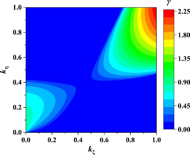
Figure 1. Diagram of the growth rate as a function of kξ and kη, where a0 = 1.0, b0 = 1.0 and k2=${{k}_{\xi }}^{2}$+${{k}_{\eta }}^{2}$. |
In figure 2, the results show that γ increases steadily with k, reaching its maximum at moderate k values, indicating that shorter wavelength perturbations enhance the modulational instability of the dusty plasma. In contrast, γ decreases gradually as ν increases, implying that higher electron-to-dust density ratios weaken the instability. This occurs because increasing ν reduces the effective nonlinear coupling between dust grains and plasma species, leading to diminished energy localization. The overall γ(k, ν) distribution thus reveals that modulational instability is strongest at small ν and moderate k, where nonlinearity dominates dispersion. The increase of γ with k results from enhanced nonlinear modulation at shorter wavelengths, while its reduction with ν reflects weakened dust-electron electrostatic coupling as electron density grows. This indicates that modulational instability is mainly controlled by the balance between nonlinear self-focusing and dispersive effects, with maximum instability occurring under strong nonlinearity and weak plasma screening. The γ(k, ν) dependence provides a theoretical basis for controlling modulational instability in laboratory dusty plasmas. By adjusting the wave number and density ratio, one can regulate instability growth, enabling stable plasma operation or controlled nonlinear modulation for applications in wave localization, plasma diagnostics, and energy confinement studies.
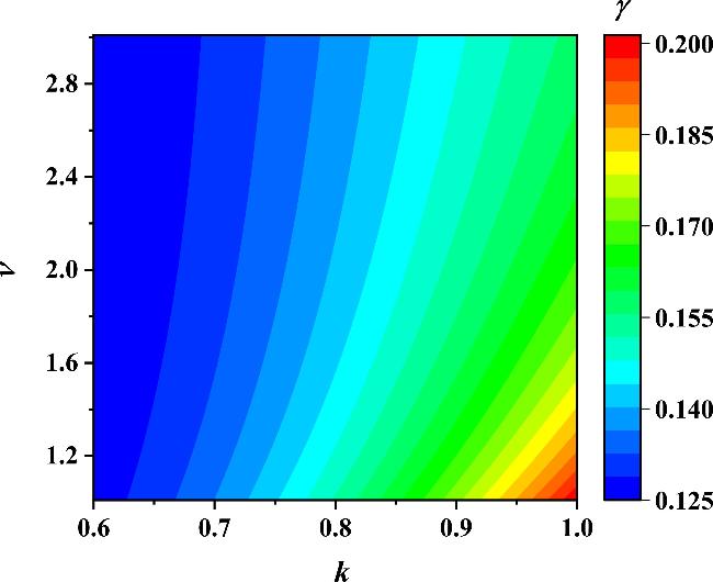
Figure 2. Diagram of the growth rate as a function of the wave number k and ν, where μ=1+ν, β = Ti/Te=1, a0 = 0.2, b0 = 0.5, kξ = $k\cos \theta $, kη = $k\sin \theta $ and θ=60∘. |
In figure 3, the results show that γ increases monotonically with k, reaching higher values at larger wave numbers, which indicates that shorter wavelength perturbations enhance the modulational instability. In contrast, γ decreases progressively with increasing β, implying that as the ion temperature rises relative to the electron temperature, the instability weakens. This inverse dependence on β reflects a reduction in nonlinear coupling strength under hotter ion conditions. The rise of γ with k originates from the strengthening of nonlinear modulation at shorter wavelengths, while its decrease with β reflects reduced dust-ion coupling as ion thermal motion increases. Hence, the modulational instability is governed by the interplay between dispersive effects and temperature-dependent nonlinearity, with maximum instability occurring when electron dominance enhances self-focusing and energy localization within the wave envelope. This functional dependence provides experimental guidance for controlling instability through plasma temperature adjustment and wavelength selection. By tuning β and k, one can suppress or enhance modulation growth, offering potential for precise manipulation of nonlinear wave structures and for optimizing plasma-based wave control and diagnostic experiments.
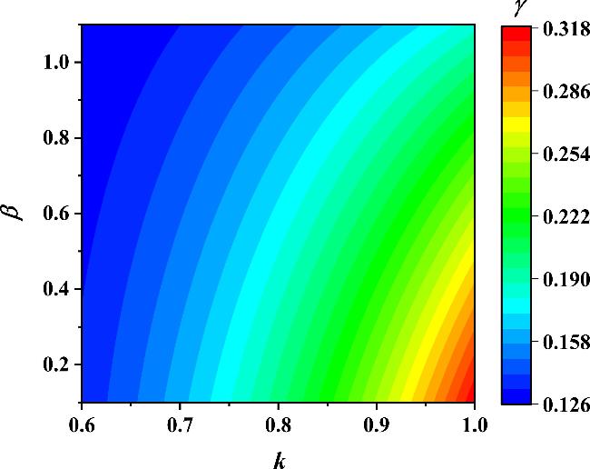
Figure 3. Diagram of the growth rate as a function of the wave number k and β, where μ=1+ν, ν=1.04, β = Ti/Te, a0 = 0.2, b0 = 0.5, kξ = $k\cos \theta $, kη = $k\sin \theta $ and θ=60∘. |
In figure 4, the figure demonstrates that γ decreases gradually as both ν and β increase. A higher ν, representing a greater ion-to-dust density ratio, weakens the nonlinear coupling between charged dust grains and plasma particles, thereby reducing instability growth. Similarly, as β increases, corresponding to higher ion temperature relative to electrons, the modulational instability diminishes due to enhanced dispersive effects and weakened electrostatic binding. The overall γ(ν, β) surface clearly indicates that instability is strongest at low ν and β values. The decreasing trend of γ with ν and β reflects the stabilizing influence of higher ion temperature and ion concentration. These conditions increase thermal dispersion and reduce charge separation, thereby weakening nonlinear self-focusing. The system thus transitions from a strongly unstable to a weakly modulated state as dust-ion coupling becomes less effective. This dependence provides experimental guidance for stabilizing dusty plasmas by adjusting density and temperature ratios. Proper control of ν and β allows suppression of envelope modulation, offering potential applications in plasma confinement, wave stabilization, and in tailoring nonlinear propagation characteristics in laboratory and space plasma environments.
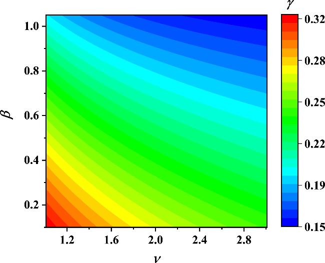
Figure 4. Diagram of the growth rate as a function of ν and β, where μ=1+ν, β = Ti/Te, a0 = 0.2, b0 = 0.5, kξ = $k\cos \theta $, kη = $k\sin \theta $, and θ=60∘. |
Figure 5 exhibits a smooth, continuous, and monotonic increase in ωr as both kξ and kη increase, without abrupt fluctuations. Specifically, in the low-wave number region (small kξ and kη), ωr approaches zero here, dispersive effects dominate over weak nonlinear coupling, and the sparse spatial distribution of dust grains weakens electrostatic interactions, leading to minimal frequency modulation. In the moderate-wave number region, ωr rises approximately linearly with the enhancement of kξ and kη: shorter wavelengths intensify the local electric field gradients around dust grains, strengthening the nonlinear coupling between dust, ions, and electrons, while the low ion temperature (β = 0.1) suppresses ion thermal diffusion, preserving the coherence of wave modulation. In the high-wave number region, the increasing trend of ωr persists but becomes gentle, as the saturation of electrostatic coupling (due to finite dust grain size and charge screening) balances the further enhancement of nonlinear effects, reflecting a systematic positive correlation between the modulation frequency and the longitudinal/transverse wave number components. This functional relationship originates from the intricate interplay between nonlinear coupling and dispersive effects: larger kξ and kη correspond to shorter wavelengths that compress the plasma medium, amplifying the electrostatic interactions among charged species. With β = 0.1, electron thermal motion is relatively dominant, which reinforces the nonlinear self-focusing of the wave envelope and enhances the energy transfer between the wave and plasma particles, thereby elevating the wave packet's modulation frequency. This finding guides experiments to precisely regulate the wave packet modulation frequency by adjusting kξ and kη under fixed plasma parameter conditions, and supports the interpretation of space plasma fluctuations while optimizing nonlinear wave modulation control in plasma diagnostic systems.
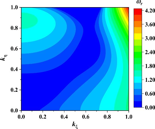
Figure 5. Dependence of the modulation frequency ωr on kξ and kη, where μ=1+ν, ν=1.04, β = Ti/Te=0.1, a0 = 1.0, b0 = 1.0 and k2=${{k}_{\xi }}^{2}$+${{k}_{\eta }}^{2}$. |
In figure 6, the curves exhibit a clear increasing trend of ωr with k, indicating that the modulation frequency rises monotonically as the wave number grows. For small k, ωr approaches zero, corresponding to the long-wavelength limit where dispersion effects dominate. As k increases, ωr grows approximately linearly at first, followed by a nonlinear saturation tendency at larger k, suggesting that dispersion becomes less significant and nonlinear coupling prevails. The magnitude of ωr also increases with the density ratio ν, implying that higher electron-to-dust density ratios enhance the modulation frequency of the wave packet. Among the three curves, the one corresponding to ν = 100.1 reaches the largest ωr, while the curve for ν = 1.1 remains lowest across all k. Thus, figure 6 quantitatively demonstrates that both the wave number and density ratio strongly influence the modulation frequency in dusty plasmas. Physically, the increase of ωr with k indicates that shorter wavelength perturbations propagate with higher modulation frequencies due to stronger nonlinear and dispersive coupling.
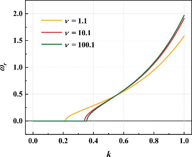
Figure 6. Dependence of the modulation frequency ωr on the wave number k at different values of ν = 1.1, 10.1, 100.1, where μ=1+ν, β = Ti/Te=0.1, a0 = 0.5, b0 = 0.2, kξ = $k\cos \theta $, kη = $k\sin \theta $ and θ=60∘. |
In figure 7, for all β values, ωr increases monotonically with k–approaching zero at low k, growing linearly in the intermediate range. β = 0.1 yielding the lowest ωr and β = 1.0 the highest within the high-k range. Physically, larger k (shorter wavelengths) strengthens electrostatic coupling among plasma species to enhance nonlinear modulation, while higher β (stronger ion thermal motion) intensifies dispersive effects, weakening nonlinear coupling. This relationship guides experiments to tune ωr via adjusting k and β, and supports plasma wave control, energy confinement optimization, and interpretation of space plasma fluctuations.
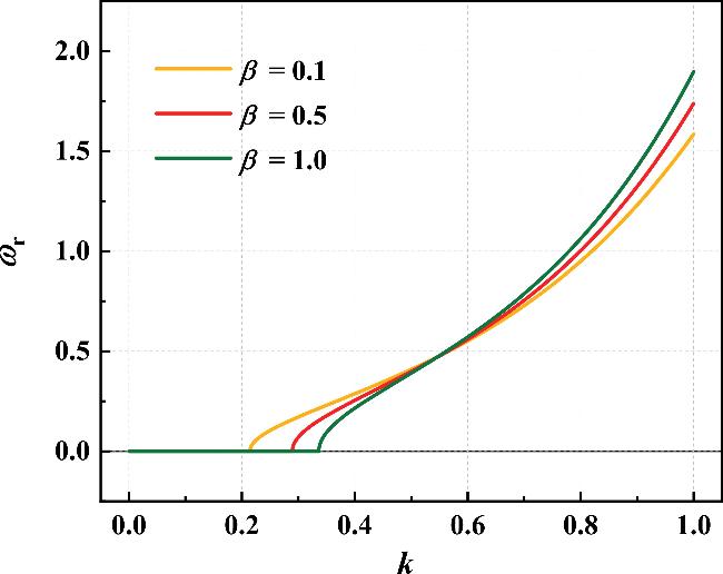


Figure 7. Dependence of the modulation frequency ωr on the wave number k at different values of β = 0.1, 0.5, 1.0, where μ=1+ν, ν = 1.1, β = Ti/Te, a0 = 0.5, b0 = 0.2, kξ = $k\cos \theta $, kη = $k\sin \theta $, and θ=60∘. |
6. Conclusion
This paper investigates multidimensional nonlinear modulation and stability of weakly two-dimensional wave packets in dusty plasma systems. The higher-order transverse perturbations of modulated wave packets in a dusty plasma are analyzed to explore the nonlinear modulation dynamics and stability characteristics. Using the DS equation which can describe the nonlinear evolution of dust acoustic waves, we analytically determine both the dispersion relation and modulational instability condition. The real and imaginary parts of the perturbed frequency, representing the modulation frequency (ωr) and the instability growth rate (γ), are then systematically examined as functions of key plasma parameters. In the first aspect, the growth rate γ is studied with respect to the wave number k, density ratio ν, and temperature ratio β. In the first aspect, the investigation of the relationship between the growth rate γ and key plasma parameters—wave number k, density ratio ν, and temperature ratio β—demonstrates that γ exhibits a substantial increase with increasing k, reaching its maximum in the intermediate wave number range. This trend arises from shorter modulation wavelengths that enhance electrostatic coupling among dust grains, ions, and electrons, thereby amplifying nonlinear modulation effects. Conversely, γ shows a gradual reduction with the elevation of both ν and β, indicating that a higher electron density fraction or stronger ion thermal motion suppresses modulational instability by weakening nonlinear coupling and reinforcing dispersive stabilization. The maximum growth of γ occurs under conditions of intermediate k and low ν and β, where nonlinear effects dominate over dispersive effects. In the second aspect, the modulation frequency ωr is systematically analyzed as a function of k, ν, and β. Notably, ωr displays a monotonically increasing trend with k: it approaches zero in the low-wave number region, grows approximately linearly in the intermediate wave number range, and the growth tends to saturate gently in the high-wave number region. Furthermore, ωr increases significantly with ν, as a higher electron-to-dust density ratio strengthens the frequency modulation of the wave packet. In the high–k region, the larger the β, the higher the ωr, as the enhanced electrostatic coupling of plasma due to short wavelengths offsets the dispersive effects caused by high ion temperatures. This work provides the theoretical guidance for controlling modulational instability and frequency modulation in dusty plasmas, thereby enriching the understanding of nonlinear wave evolution in complex plasma systems.