


1. Introduction
Magnetic reconnection is a natural process in plasma physics that can trigger various instabilities. It plays a crucial role in energy redistribution within plasmas and contributes to the development of different types of instabilities [1–7]. This phenomenon involves changes in the structural characteristics of the magnetic field along with the conversion of magnetic energy into thermal and kinetic energy. In space and laboratory plasmas, magnetic reconnection is known to be the origin of many natural phenomena, such as solar flares [8, 9], geomagnetic storms [10], and sawtooth crashes in tokamak [11, 12]. Magnetic reconnection [13] and plasma turbulence [14–16] are fundamental processes responsible for transferring energy across different scales and between electromagnetic fields and particles [17, 18]. Furthermore, a dynamic interplay exists between magnetic reconnection and turbulence, not only can reconnection drive turbulence [19, 20], but small-scale reconnection events are also frequently embedded within turbulent environments [21]. The configuration of the magnetic field plays a crucial role in both phenomena. In a two-dimensional framework, reconnection occurs within structures and interactions governed by topological constraints. In a turbulent environment, multiple reconnection X-lines can form simultaneously [22]. In this particular two-dimensional flow, magnetic flux islands interact, generating thin current sheets [23]. In addition to numerical simulations, similar magnetic islands have also been observed by spacecraft [24]. These sheets then undergo reconnection, driving magnetic merging and contributing to the development of coherent structures [25, 26]. A reconnection current layer is naturally unstable and tends to fragment into multiple secondary magnetic islands and current filaments [27, 28], even within a smooth flow. These processes have been identified through both numerical simulations [27, 29] and direct in-situ observations [30, 31]. Unlike its two-dimensional counterpart, three-dimensional reconnection exhibits significant differences due to the presence of turbulence [22, 32, 33] and intrinsic asymmetries in the reconnecting current sheet [34, 35]. Advanced kinetic simulations of three-dimensional reconnection reveal a complex network of flux ropes [36–38] and outflow regions that can evolve into turbulence [39]. These processes include turbulence in a fast-moving outflow or result from the formation and interaction of multiple X-lines or magnetic null points.
The boundary layers of Earth's magnetotail contain strong current densities, with distinct regions exhibiting magnetic fields of varying magnitudes and orientations, commonly referred to as current sheets [40, 41]. Unstable phenomena, such as magnetic reconnection, can occur within these sheets, leading to the release of stored energy. As a result, current sheets are fundamental to the behavior of space plasmas, exhibiting a distinctive magnetic field configuration that corresponds to the underlying current system. In reality, current sheets in space have highly intricate structures, and observations indicate that current density is primarily concentrated in their narrow central region [42]. Magnetotail current sheets can be extremely thin and may exhibit a bimodal or trimodal distribution of current density. Typically, the magnetotail current sheet contains a By component of the magnetic field, which can result from the penetration of the interplanetary magnetic field into the magnetosphere. The observed flat current sheet (FCS) differs markedly from the conventional current sheet reported by Shen et al [43], in which only a weak duskward magnetic field component (By) is present at the neutral sheet. In contrast, the current sheet analyzed here is characterized by a pronounced guide field at the neutral sheet, while the north–south magnetic component (Bz) remains comparatively weak. This combination of magnetic features gives rise to an atypical current sheet configuration. Owing to its distinct magnetic structure, we classify this configuration as a FCS. During a substorm event, the structure of the magnetic field and the distribution of the magnetotail current sheet characterized by a strong guide field component (By) were examined by [44]. The magnetic field lines (MFLs) within this current sheet predominantly lie in the equatorial plane of the geocentric solar magnetospheric (GSM) coordinate system, with the normal vector typically oriented in the northward direction. The MFLs do not form a simple planar curve; instead, for By > 0, they create a left-handed spiral, whereas for By < 0, they form a right-handed spiral. The MFLs quickly change direction in neutral sheet's regime. In the course of the substorm evolution phase, the neutral sheet gradually becomes thinner, while the current density tends to increase [44]. This study focuses on utilizing a multi-point satellite data analysis approach to examine and reconstruct the MFLs, their spatial geometry, helix angle, and torsion of the FCS having flat geometry. The analysis is conducted using the GSM coordinate system.
The curvature, which reflects the rate at which the direction of a magnetic field changes at a specific point, is an essential factor in describing the structure of MFLs [45, 46]. This parameter is closely associated with interactions between magnetic fields and matter [47], magnetic reconnection, and processes such as particle heating and acceleration [48, 49]. Researchers in magnetospheric physics, plasma and space physics have shown considerable interest in this concept. Extensive research has been dedicated to analyzing various characteristics of the magnetic field—including parameters such as field-line curvature and magnetic rotation—across distinct regions such as the ring current, current sheets, and the geomagnetic tail [43, 50–52]. Variations in magnetic field curvature significantly influence the trajectories of charged particles within different magnetospheric environments. Numerous investigations have demonstrated that this phenomenon is a key contributor to the reduction of high-energy particle populations within the ring current and the proton radiation belt [53–56]. Although progress has been made, the understanding of how curvature behaves within a turbulent magnetic field is still evolving, and its precise influence on particle dynamics under such conditions remains an open area of investigation [57].
Structured patterns are commonly observed in both astrophysical and laboratory plasma turbulence [16, 58, 59]. Even in the case of homogeneous and isotropic hydrodynamic turbulence, localized vortex formations can intermittently arise [60]. As a system of plasma turbulence, the solar wind has been extensively studied with regard to its magnetic field structure, including the investigation of field discontinuities [61], current sheets [62], and neutral X-lines [63]. The breakdown of the magnetic frozen-in condition typically occurs at X-lines, where MFLs disengage from the motion of the plasma. This process is closely linked to the energization of charged particles [64]. Simulations have shown that organized current sheet structures exist across multiple scales and play a vital role in particle heating and energy dissipation [65]. Discontinuities in the solar wind serve as key drivers of turbulence within the magnetosheath and significantly affect the manner in which the solar wind couples with the magnetosphere [61]. Nevertheless, not all structured features actively participate in the processes of energy transfer or dissipation. Certain magnetic field configurations—specifically those that are force-free, where the magnetic field is aligned with the current density, can maintain stability and drift passively with the plasma flow [66]. Understanding the nature of magnetic field geometries is essential for uncovering the mechanisms behind plasma turbulence within the magnetosheath. Moreover, the magnetic field gradient tensor significantly influences the governing equations that dictate the behavior of turbulent velocity fields, and thus warrants detailed analysis.
This research primarily examines the development of magnetic field structures defined by curvature, torsion, and helix angle within FCSs. Additionally, we aim to analyze the characteristics of these FCSs, which have varying By, using nonlinear magnetic field gradient analysis (NMG). We will employ the geometric characteristics of the magnetic field gradient to analyze the local structural properties both quantitatively and qualitatively. Section 2 outlines the data and methodology applied in this study, while sections 3 and 4 present the results and the summary, respectively.
2. Data
The first event selected for the study was observed by the magnetospheric multiscale (MMS) satellite from 12:18:00 to 12:19:30 UT on August 10, 2017. The position of the MMS satellite at this time is [−15.2, 2.6, 4.8] RE, located at the magnetotail position, and is moving from the tail towards Earth. The second event selected for the study occurred from 08:31:00 to 08:32:00 UT on July 6, 2017. The position of the MMS satellite at this time is [−22.1, 2.2, 3.6] RE, located at the magnetotail position, and is moving towards the tail in the direction away from the Earth.
3. Method
3.1. Theory and geometrical parameters
In a previous study [67], we detailed the mechanism of a magnetic flux entanglement event. The MMS satellite was positioned close to the magnetospheric apex and was moving inward toward the inner side of the magnetopause. The distinct observed phase was discussed near the magnetopause. The fluxgate magnetometers on the four spacecraft measured the three components of the magnetic field in the GSE coordinate system. Flux tube entanglement events are frequent and commonly occur at the magnetopause. The acquired data corresponds to equilibrium states, which are analyzed in this study. These states are uniquely determined by the thermal plasma pressure contained within the magnetospheric cavity. The characteristic time and length scales are estimated under the assumption that the boundary conditions of the magnetopause and solar wind remain constant. To investigate the diffusion of the magnetic field leading to reconnection in magnetic flux tubes, we examined equilibrium states in a highly simplified two-dimensional magnetosphere, as detailed in [67]. In this study, we consider that all physical quantities vary based on the x and z coordinates within the GSM system. The Earth's magnetic dipole lies within the noon–midnight plane of the magnetosphere, which corresponds to the x–z plane, with the x-axis pointing in the direction of the Sun. In a two-dimensional framework, the magnetic field components can be derived from a flux function, ψ(x, z), which defines the magnetic field distribution at given coordinates. When the plasma has zero resistivity, the magnetic field does not penetrate it, except at boundaries where one region contains plasma without a magnetic field and another has a magnetic field without plasma—such as in the interplay between the Earth's magnetic field and solar wind. In this scenario, plasma influences the magnetic field by pushing, bending, and twisting field lines as it moves. However, when resistivity is nonzero, the plasma and magnetic field can permeate each other. It requires some time for this diffusion to occur, and if the motions are slow enough, the plasma motions will not have to deform the field lines. To determine the diffusion of the magnetic field during a solar wind interaction event, Ampere's and Faraday's laws are used, as given below, 1 ) due to neglecting fast oscillations. These equations are coupled, and to decouple them, we assume the microscopic version of Ohm's law E = ηj, by taking into account plasma in the solar wind interacts with Earth's magnetic field. By simultaneously solving equations (1 ) and (2 ), we get 3 ) can be solved by applying the separation of variables technique. To obtain an approximate estimate, we consider L as the characteristic length scale of the spatial variation of B. Consequently, the solution for magnetic field diffusion is given as
$\begin{eqnarray}{\rm{\nabla }}\times {\boldsymbol{B}}={\mu }_{0}{\boldsymbol{j}},\end{eqnarray}$
$\begin{eqnarray}{\rm{\nabla }}\times {\boldsymbol{E}}=-\frac{\partial {\boldsymbol{B}}}{\partial t},\end{eqnarray}$
where, we have ignored displacement term in equation ( $\begin{eqnarray}\frac{\partial {\boldsymbol{B}}}{\partial t}=-\frac{\eta }{{\mu }_{0}}\left[{\rm{\nabla }}({\rm{\nabla }}\cdot {\boldsymbol{B}}-{{\rm{\nabla }}}^{2}{\boldsymbol{B}})\right],\end{eqnarray}$
where, η = 5.2 × 10⁴ lnΓ/(kT)3/2 is Spitzer resistivity and lnΓ = 10 has been implemented for the solar wind. The magnetic diffusion equation ( $\begin{eqnarray}{\boldsymbol{B}}={{\boldsymbol{B}}}_{{\bf{0}}}{\rm{\exp }}[\pm \eta t/{\mu }_{0}{L}^{2}].\end{eqnarray}$
In this context, L represents the characteristic spatial scale over which the magnetic field penetrates the plasma. The magnetic field components are expressed in the GSM coordinate system, as detailed in equation (2) of the [67]. The contour plots for the diffusion profile of Earth's magnetic field at different characteristic length scales $\hat{r}=L/{R}_{E}$ (a) at $\hat{r}\lt 1$, (b) $\hat{r}=1$, (c) $\hat{r}=3$ and (d) $\hat{r}=5$ are shown in figure 1. Panels (a–d) show contour maps of the magnetic field magnitude as a function of position at different values of characteristic length (a) $\hat{r}\lt 1$ illustrates the strongest spatial gradients and the most rapid magnetic field diffusion near, (b) $\hat{r}=1$ demonstrates that diffusion becomes less steep but still significant, (c) $\hat{r}=3$ represents weaker gradients and slower diffusion at outer magnetospheric regions and (d) $\hat{r}=5$ very weak magnetic diffusion corresponding to distant tail regions. The magnetic field diffusion varies with scale length and serves as a theoretical foundation for understanding the sensitivity of quadratic magnetic gradients in flat current-sheet analysis. The dynamics of Earth's magnetic field vary with distance and depends on the characteristic length scale over a specific period of time. We adopted the normalized time interval of event as discussed in our earlier paper [67]. The findings suggest that both the estimation of quadratic magnetic gradients and the spatial configuration of MFLs are essential for analyzing magnetic structures in space plasmas through multi-point observations. These estimators demonstrate high accuracy when compared to theoretical models. The formulation summarized above can serve as a basis for the actual calculation stages. The magnetic field for the two-dimensional magnetic configuration can be expressed using the physical insight from figure 1. A small characteristic length scale $\hat{r}$ causes the magnetic field to dissipate more rapidly, giving the appearance of a smaller spatial range in figure 1(b). The magnetic gradients in figure 1(a) are steeper, which leads to faster spatial diffusion even if the diffusion coefficient is numerically smaller. Subsequent panels with larger diffusion coefficients exhibit weaker but broader diffusion rather than sharper decrease. The parametric analysis of the current sheet according to observations of the background magnetic field B0 ≈ 1–5 nT, and distances are in terms of the characteristic normalized length scale $\hat{r}$ are shown in figure 2. The solid black curve is plotted at characteristic length $\hat{r}=1$ which represents the strong variation of the current sheet near the Earth in the magnetospheric environment, while all other dotted (or dashed–dotted) curves are generated at larger distance of $\hat{r}$ represents the weak profile of current sheets in the outer region of magnetosphere of the Earth. Figure 3 illustrates a hypothetical trajectory for the spacecraft (S/C) constellation, beginning at coordinates (−1, 1)RE and extending to (−3, −1)RE. The constellation is modeled as a regular tetrahedron with an inter-spacecraft separation of 100 km. Panels (a) and (b) in figure 3 present the analytical values of the magnetic field in GSM coordinates at the barycenter of the four spacecraft. In 2D MHD equilibria the quantity δ2 = α2 − K2 − H2 retains the set of parameters by which the equilibrium model is established [68], where, α = (2n − 1) is corresponding eigenvalue, K and H are constant scaling factors. In this analysis, the first eigenvalue is selected as α = π/2 to assess the magnetic field's spatial gradient at the constellation's center. The propagation of the magnetic field associated with the nonzero components Bx and Bz of the linear magnetic gradient at the barycenter, as shown in figures 3(c) and (d), is determined using equation (4 ). The red solid lines indicate the analytical results obtained using the theoretical formula. The star, filled square, and filled circle on the lines are representing the characteristic distances $\hat{r}=1$, $\hat{r}=2$ and $\hat{r}$ = 3, respectively. The second gradient, as shown in figures 3(e) and (f), results from applying the linear magnetic gradient to determine the quadratic magnetic gradient within the current sheet framework. In this model, Bx and By correspond to the quadratic variations of the magnetic unit vectors, while only Bz retains a nonzero value. As illustrated in figure 3, Bx exhibits a bipolar pattern centered around the middle of the current sheet, reaching zero at the midpoint. In contrast, Bz displays symmetry along the left–right axis, with peak magnetic field diffusion observed at the normalized characteristic length $\hat{r}=1$. The changes observed in the curvature and torsion of MFLs suggest that the magnetic topology is distinct from that of the current sheet. Notably, the central regions of these field lines exhibit peak torsion and reduced curvature. As the MFLs approach the core of the flux rope, they become increasingly twisted and aligned, indicating that the structure of the flux rope is helical and three-dimensional in nature. In this study, the magnetic flux ropes are embedded within the reconnection exhaust adjacent to the magnetopause current sheet. They are identified during the time intervals marked by the vertical red lines, where the magnetic field exhibits a coherent rotation in the transverse components (Bx, By, Bz) accompanied by a localized enhancement in the total magnetic field magnitude (Bt). These magnetic signatures are coincident with modest but noticeable variations in plasma density and pressure, indicating the passage of magnetically dominated structures rather than purely compressional features. In the 06-07-2017 event, the flux rope is encountered shortly after the current sheet crossing, suggesting formation close to the reconnection site. In contrast, the 10-08-2017 event shows flux-rope encounters within an extended exhaust region, implying the presence of evolving or coalescing structures downstream of reconnection. The consistent alignment of the magnetic rotation across all MMS spacecraft further confirms that these flux ropes are spatially coherent, ion-scale structures embedded within the reconnection outflow on the magnetosheath side of the dayside magnetopause. The upcoming sections detail the computed curvature and torsion of the MFLs within the current sheet. The torsion remains nearly uniform across the examined segments, suggesting that the MFLs are largely confined to a plane—an observation consistent with theoretical expectations.
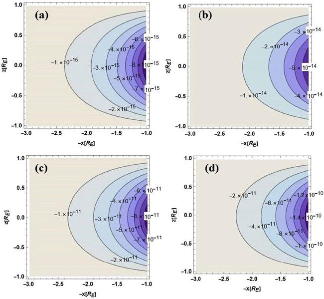
Figure 1. Analytical diffusion profile of Earth's magnetic field in terms of magnetic flux function ψ derived from the magnetic diffusion equation ( |
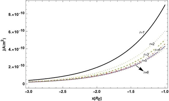
Figure 2. Parametric analytical model of the magnetic field configuration within an idealized current sheet for different characteristic normalized length scales $\hat{r}=L/{R}_{E}$. The solid black curve represents the magnetic field variation at $\hat{r}=1$, corresponding to a region closer to Earth where the current sheet exhibits the strongest curvature and sharpest magnetic-gradient transitions. The dashed and dashed–dotted curves represent higher values. |
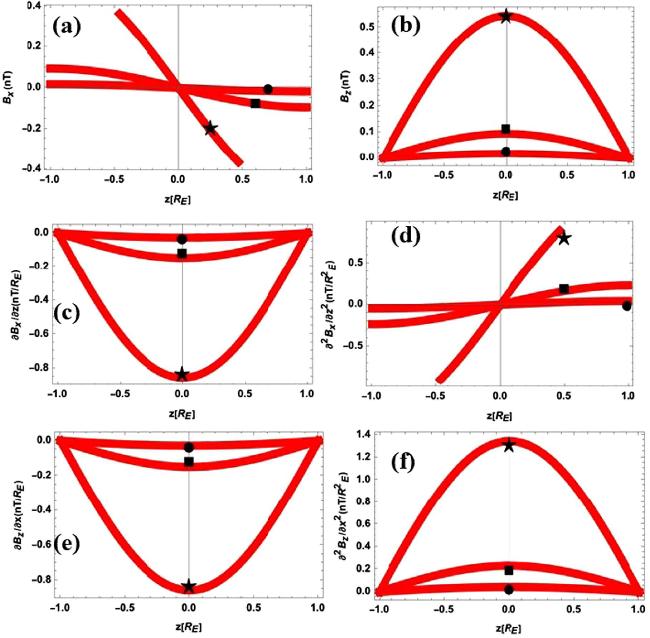
Figure 3. Variation of magnetic field strength along (a) Bx, (b) Bz, linear magnetic gradient of (c) Bx, (d) Bz, and quadratic magnetic gradient of (e) Bx, (f) Bz with respect to characteristic length scale $\hat{r}$. The red solid lines indicate the analytical results obtained using the theoretical formula. While, the star, the filled square and the filled circle on the lines are representing the characteristic distances at $\hat{r}=1$, $\hat{r}=2$ and $\hat{r}=3$, respectively. |
Next, we examine the mathematical expressions that characterize the geometric structure of the magnetic field, with particular attention to the curvature, helical angle, and torsion of its field lines, as well as the geometric invariants linked to the magnetic field gradient. The curvature vector quantifies how the direction of the magnetic field changes along its path, and its formal definition is provided below,
$\begin{eqnarray}\kappa =\left|{\boldsymbol{b}}\cdot {\rm{\nabla }}{\boldsymbol{b}}\right|.\end{eqnarray}$
In equation (5 ), the vector κ represents the curvature, while the unit vector ${\boldsymbol{b}}=\frac{{\boldsymbol{B}}}{B}$ indicates the direction of the magnetic field, where B denotes the magnetic field vector and B its magnitude. An alternative formulation of equation (5 ) can also be expressed as;
$\begin{eqnarray}\kappa =\frac{\left|{\boldsymbol{b}}\times \left({\boldsymbol{B}}\cdot {\rm{\nabla }}{\boldsymbol{B}}\right)\right|}{{B}^{2}}.\end{eqnarray}$
The expression ${{\boldsymbol{f}}}_{{\boldsymbol{n}}}={\boldsymbol{b}}\times \left({\boldsymbol{B}}\cdot {\rm{\nabla }}{\boldsymbol{B}}\right)$ denotes the magnetic tension force per unit volume, oriented orthogonally to the MFLs. In addition, the MFLs exhibit a helical structure, the extent of which is characterized by the torsion, formally defined as follows,
$\begin{eqnarray}\tau =\frac{1}{\kappa }\frac{{{\rm{d}}}^{2}{\boldsymbol{b}}}{{\rm{d}}{s}^{2}}\cdot {\boldsymbol{N}}=\frac{1}{\kappa }\frac{{\rm{d}}{\boldsymbol{\kappa }}}{{\rm{d}}s}\cdot {\boldsymbol{N}}=-\frac{1}{\kappa }{\boldsymbol{\kappa }}\cdot \frac{{\rm{d}}N}{{\rm{d}}s}.\end{eqnarray}$
The subnormal vector of a MFL, denoted as N = b × K, where K = κ/κ represents the principal normal vector of the MFL. Furthermore, the expression for τ can be written as follows
$\begin{eqnarray}\begin{array}{rcl}{\boldsymbol{\tau }} & = & {\kappa }^{-1}{B}^{-3}{N}_{{j}}{B}_{{i}}\left({{\rm{\nabla }}}_{{i}}{B}_{{k}}\right)\left({{\rm{\nabla }}}_{{k}}{B}_{{j}}\right)\\ & & +{\kappa }^{-1}{B}^{-3}{N}_{{j}}{B}_{{k}}{B}_{{i}}\left({{\rm{\nabla }}}_{{k}}{{\rm{\nabla }}}_{{i}}{B}_{{j}}\right).\end{array}\end{eqnarray}$
In the given context, the symbols i, j, k represent directions in a Cartesian coordinate system. Here the magnetic field's first and second order gradient are represented by the terms ∇iBk, ∇kBj, and ∇k∇iBj respectively. If we know the torsion τ and curvature κ of the cylindrical spiral MFLs the helix angle can be written as ${\rm{\tan }}\beta =\frac{\tau }{\kappa }$, here β represents the helix angle. Also, the azimuthal angle can be expressed by $\phi =\frac{{\rm{\cos }}\beta }{r}s$. The discussion of magnetic field properties and topologies can be expanded to incorporate magnetic field gradients, in addition to curvature and torsion. The geometric invariants of ∇B determine both the local quantitative and qualitative characteristics of the MFL topologies. Here, geometrical invariants mean the quantity or property of a geometrical object that remains unchanged during a specific transformation. These geometrical invariants consist of three scalars that remain unchanged when the frame undergoes a rotation operation. In this case the geometrical invariants can be defined as,
$\begin{eqnarray}\begin{array}{rcl}P & = & -{\rm{t}}{\rm{r}}\left({\rm{\nabla }}{\boldsymbol{B}}\right),\quad Q=-\frac{1}{2}{\rm{t}}{\rm{r}}\left({{\rm{\nabla }}}^{2}{\boldsymbol{B}}\right),\\ R & = & \frac{1}{3}{\rm{t}}{\rm{r}}\left({{\rm{\nabla }}}^{3}{\boldsymbol{B}}\right).\end{array}\end{eqnarray}$
In this context, the absence of magnetic field divergence leads to P = 0. It should be noted that geometric invariants are represented by the polynomial coefficients in the characteristic equation ∣∇B − λiI∣ = ${\lambda }_{{i}}^{3}+P{\lambda }_{{i}}^{2}+Q{\lambda }_{{i}}+R=0$. It can be demonstrated that $D=\frac{27}{4}{R}^{2}+{Q}^{3}$ dictates the nature of solutions λi in the (R, Q) plane. When D > 0, λi consists of two complex numbers and one real number; conversely, when D < 0, all λi are real. The real and complex λi correspond to distinct topologies of MFLs.
3.2. Nonlinear magnetic field gradient algorithm
For the analysis of the geometrical parameters of different magnetic structures, the essential step involves calculating the magnetic field gradients, as detailed in the preceding section. We utilize an advanced multipoint method, the NMG algorithm, recently developed by [69]. This algorithm enables the determination of both first and second-order magnetic field gradients, encompassing 9 and 18 parameters, respectively. Additionally, NMG enables the calculation of the apparent velocity (3 parameters) and magnetic field (3 parameters) structures. It is important to emphasize that the determination of these physical quantities relies on the barycenter of the spacecraft constellation. However, determining all 33 parameters necessitates applying specific physical constraints, as the data collected by the S/C only provide information on the current density and different magnetic fields vectors, which alone are inadequate for full determination. NMG incorporates various physical constraints in its calculations, ensuring a comprehensive and accurate evaluation of the parameters.
the transformation relationships:
$\begin{eqnarray}\frac{\partial {\boldsymbol{B}}}{\partial t}=-{\boldsymbol{V}}\cdot {\rm{\nabla }}{\boldsymbol{B}},\quad \partial \frac{{\rm{\nabla }}{\boldsymbol{B}}}{\partial t}=-{\boldsymbol{V}}\cdot {\rm{\nabla }}{\rm{\nabla }}{\boldsymbol{B}},\end{eqnarray}$
formula from Ampere's law: $\begin{eqnarray}{\rm{\nabla }}\left({\rm{\nabla }}\times {\boldsymbol{B}}\right)={\rm{\nabla }}{\boldsymbol{j}},\end{eqnarray}$
formula from the solenoidal condition: $\begin{eqnarray}{\rm{\nabla }}\left({\rm{\nabla }}\cdot {\boldsymbol{B}}\right)=0,\end{eqnarray}$
equation derived from magnetic rotation analysis (MRA): $\begin{eqnarray}\frac{\partial }{\partial {X}_{3}}\frac{\partial }{\partial {X}_{3}}{b}_{p}=0.\end{eqnarray}$
In the context where X3 represents the direction along the MFL and p = 1, 2 signifies two additional characteristic directions in the local MRA coordinate system, it is essential to highlight that [69] have introduced an iterative approach to enhance the precision of the quadratic magnetic gradient determination. Additional information on NMG can be found in the publication by [69].
4. Results
4.1. First event
Figures 4 and 5 show the current sheet crossing event, during the period 12:18:00 to 12:19:30 on UT 2017-08-10, also this event was reported by Zhou [70]. The MMS satellite traversed the magnetotail plasma sheet twice, moving from the southern hemisphere to the northern hemisphere, before crossing back into the southern hemisphere. These figures also present the magnetic field profiles across the thin current sheet. The central region of the current sheet, referred to as the neutral sheet, is distinguished by a significantly diminished magnetic field intensity. In both figures, the boundaries of the current sheet are delineated by vertical red lines, while the midpoint is indicated by a vertical purple line. As shown in figure 4, the magnetic field components in the y-direction at the center of the sheet (marked by the purple line) are approximately By ≈ 2.03 nT and the total magnetic field magnitude is Bt ≈ 2.08 nT. A strong guide field is present at the core of the current sheet, although the Bz component remains relatively small, measuring around 0.2 nT at the neutral sheet. This type of current sheet has a unique structure, distinct from typical current sheets, and features a noticeable By guide field component at the neutral sheet location. To further analyze the area within the neutral sheet, we have transformed the data into the LMN coordinate system. In this system, N represents the normal direction of the current sheet, determined by four satellites, ${\boldsymbol{M^{\prime} }}$ corresponds to the average current direction, and L is perpendicular to both N and ${\boldsymbol{M^{\prime} }}$. The M direction is derived by applying N × L. Across these regions, the magnetic field components exhibit systematic rotations and localized depressions in the total field, indicating repeated traversals of thin, structured current sheets in the magnetotail plasma sheet. Concurrent enhancements and variations in plasma density and pressure near the sheet centers point to strong plasma–field coupling and localized compressions associated with current sheet dynamics. The close agreement among the four MMS spacecraft confirms the spatial coherence of these structures, while the repeated, layered crossings suggest a fragmented and evolving current sheet system, consistent with active reconnection and transient magnetic structuring in the near-tail environment. Within each interval bounded by the red lines, the magnetic field components undergo pronounced rotations and amplitude changes, accompanied by local minima in the total magnetic field, consistent with traversals of thin current sheets. Near the centers of these sheets, variations in plasma density and pressure become more prominent, reflecting enhanced plasma compressibility and dynamic coupling between particles and electromagnetic fields. The repeated occurrence of such signatures over a short time interval indicates multiple, closely spaced current sheet encounters, suggesting a structured and dynamic plasma sheet environment. The coherent behavior observed across the four spacecraft further implies that these current sheets possess spatial continuity on MMS inter-spacecraft scales and are likely embedded within an actively evolving reconnection region in the magnetotail.
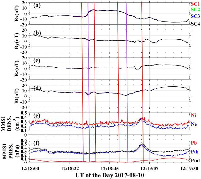
Figure 4. Changes in magnetic field strength (a) Bx, (b) By, (c) Bz, and (d) Bt, (e) electron ion density Ne, and Ni, (f) thermal pressure Pth, magnetic pressure Pb, and total pressure Pt detected by the four MMS satellites from 12:18:00 to 12:19:30 on August 10, 2017. The red vertical lines represent the boundaries of the current sheets and purple vertical lines show the center of the current sheets. |
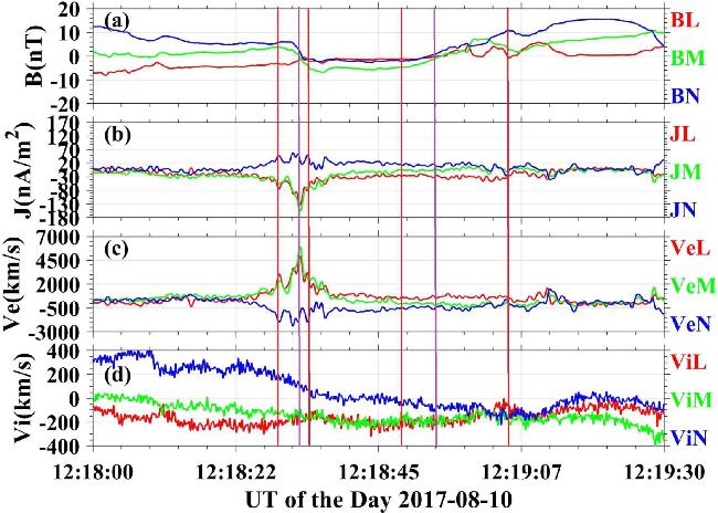
Figure 5. Changes in (a) magnetic field intensity BL, BM, and BN, (b) current density JL, JM, and JN, and (c) electron VeL, VeM, VeN, (d) ion velocities ViL, V${}_{{iM}}$, ViN of the magnetic field structure in the GSE coordinate system from 12:18:00 to 12:19:30 on August 10, 2017. The red vertical lines represent the boundaries of the current sheets and purple vertical shows the center of the current sheets. |
Figure 5 illustrates the changes in various parameters during a specific time interval on August 10, 2017, from 12:18:00 UT to 12:19:30 UT. These parameters include (a) magnetic field strength components BL, BM and BN, (b) current density components JL, JM and JN, (c)–(d) electron velocities VeL, VeM, VeN, and ion velocities ViL, V${}_{{iM}}$, ViN in the LMN coordinate system. In figures 5(a) and (b), it is clear that close to the neutral sheet, both the magnetic field strength component BN and the current density component JN undergo minimal variations in the normal direction of the current sheet, stabilizing at zero. Near-zero behavior of the normal magnetic field component (BN) and the normal current density (JN) is observed during the time interval associated with the neutral sheet crossing, approximately 12:18:30–12:18:40 UT, as marked by the vertical lines in panels (a) and (b). During this period, both quantities show only weak fluctuations about zero, indicating that the spacecraft was located close to the center of the current sheet. At times outside this interval, BN and JN exhibit larger variations, consistent with movement away from the neutral sheet. At the same time, the magnetic field strength component BM undergoes a polarity change from positive/negative to negative/positive, accompanied by a noticeable rise in current density. Figure 5(b) illustrates the spatial distribution of current density across the current sheet, indicating that the components along the M-direction and aligned with the magnetic field predominantly contribute to the total current density within the neutral sheet. Notably, the dominant current is oriented antiparallel to the magnetic field, with a maximum magnitude surpassing 170 nA m2, reflecting an unusually intense current flow. It appears that a very robust interaction occurs where the polarity reversal takes place. Examining figure 5(c) and observing the curve depicting changes in electron velocity, it is evident that as the satellite crosses the neutral sheet, there's a substantial boost in electron velocity, resulting in the observation of an ultra-Alfven electron flow. Specifically, the electron velocity reaches VeM = 6000 km s−1 in the M direction, roughly 7.6 times the Alfven speed (VA), and VeL = 5000 km s−1 in the L direction, approximately 6.3 times VA. Notably, VA, calculated at around 790 km s−1, serves as the Alfven speed. These findings strongly suggest that magnetic reconnection occurs near the neutral sheet location, yielding an exceptionally rapid electron jet. When figure 5(d) is considered alongside this, it becomes evident that the electron's velocity significantly surpasses that of the ion, establishing the electrons as the primary carrier, with acceleration and inversion occurring along the M direction. This species-dependent behavior reflects the decoupling of electron and ion dynamics on kinetic scales and is characteristic of active reconnection regions. The temporal coincidence between magnetic field rotations, peaks in current density, and enhanced electron flows provides compelling evidence that the spacecraft repeatedly encountered structured, dynamically evolving current sheets. Together, these signatures indicate that the plasma sheet in this interval was highly structured and undergoing ongoing reconfiguration, consistent with bursty reconnection and associated particle acceleration in the magnetotail.
Subsequently, the NMG algorithm is employed to compute both the primary and secondary gradients of the magnetic field. The NMG algorithm is applied to examine the current sheet crossing event, with the resulting variation curves of magnetic field curvature, helix angle, and torsion illustrated in figure 6. As depicted in figure 6(b), the curvature noticeably increases near the location of the neutral sheet. At the time when the MMS spacecraft first intersects the current sheet, the MFL curvature at the neutral sheet's center attains its peak value, with the curvature parameter κ measured at approximately 0.008 km−1. This equates to a radius of curvature (Rc) near 0.019 Earth radii, or about 125 km. As depicted in figure 6(b), the MFL on the southern flank of the current sheet initially curves northward. Upon nearing the central region, the direction of curvature and the orientation of the local normal vector vary rapidly, suggesting the presence of a helical magnetic configuration in the vicinity of the neutral sheet. As the MMS continues traversing northward through the current sheet, the curvature shifts predominantly southward. Analysis of the magnetic structure indicates that the field lines within the neutral sheet exhibit a clockwise rotation about a northward-directed normal vector, thereby forming a left-handed helical structure. The curvature reaches its maximum at the midpoint of the neutral current sheet and gradually diminishes to nearly zero elsewhere. Similarly, the graph of the helix angle reveals that the average helix angle remains close to 45° within the neutral current sheet, as shown in figure 6(c). Furthermore, the torsion exhibits the minimum variation at the mid-point of the sheet, with a maximum variation around it, as illustrated in figure 6(d). Based on this analysis, it can be concluded that the different magnetic field geometries of this sheet are not plane curves, but rather spiral curves. As seen in figure 6(c), the helix angle experiences significant variations near the neutral sheet, further indicating the spiral nature of the magnetic structures. The combined behavior of curvature, shear, and torsion demonstrates that the current sheet during this interval is neither planar nor static but instead exhibits pronounced three-dimensional deformation and temporal variability. These characteristics are consistent with an actively evolving reconnection environment, where MFLs experience strong bending, rotation, and twisting on kinetic scales.
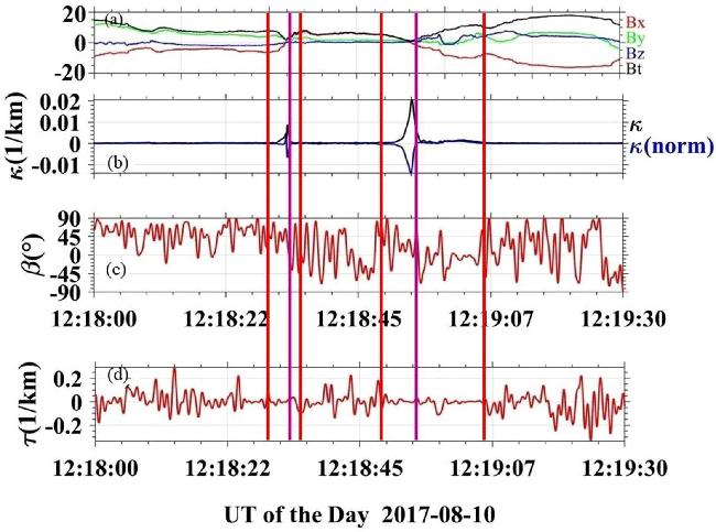
Figure 6. Variation curves of (a) magnetic field strength Bx, By, Bz, and Bt, (b) curvature, (c) helix angle and (d) torsion of the magnetic field lines calculated by the NMG algorithm during the UT period from 12:18:00 to 12:19:30 on August 10, 2017. |
As shown in figure 7, the magnetic field vector's polar angle, θB, remains relatively constant at approximately 90° throughout the current sheet crossing event, suggesting that field lines generally aligned with the equatorial plane during this time. At the central region of the current sheet, the magnetic field vector exhibits an azimuthal angle (φB) of 79° and a polar angle (θB) of 95° [figure 7(b)]. Furthermore, the graphical representation reveals a variation in φB near 180° during the current sheet's traversal, whereas θB remains relatively constant. At the midpoint of the neutral current sheet—denoted by the purple vertical line—the secondary normal vector of the magnetic field is oriented approximately southward, with a polar angle θN of 170° [figure 7(d)]. As illustrated in figures 7(e) and (f), the magnetic field's first-order gradient points southward in the lower region and northward in the upper region of the sheet, reaching a minimum at the center where the gradient reverses direction. This configuration suggests that the current sheet is nearly aligned with the equatorial plane, and its normal vector is directed northward. The coordinated changes in magnetic field direction, curvature and binormal orientations, and the intensification of ∣∇B∣ collectively indicate that the current sheets are highly structured, spatially localized, and dynamically evolving. These features are characteristic of active reconnection regions and reflect the complex three-dimensional topology of the magnetotail plasma sheet during this interval.
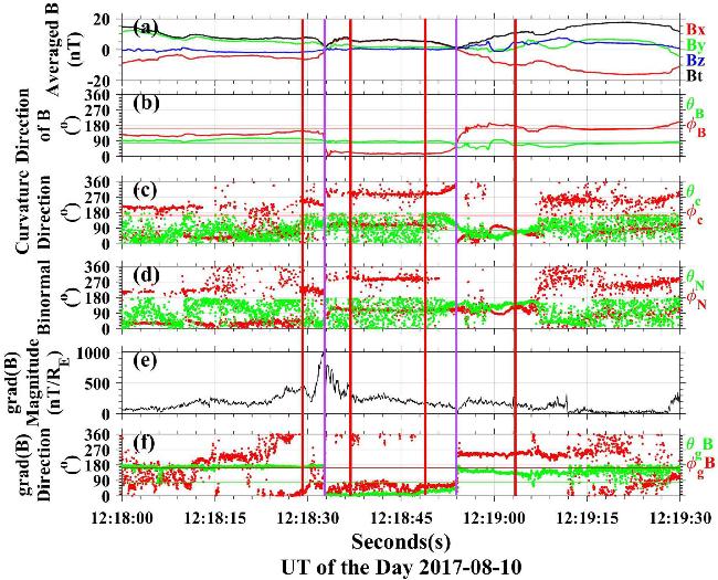
Figure 7. (a) Changes in magnetic field strength Bx, By, Bz, and Bt, (b) polar θB and azimuth φB angles of the magnetic field vector; (c) the azimuth sum of the curvature of the magnetic field lines θc and φc; (d) the azimuth θN and φN of the subnormal vector of the magnetic field lines; (e) first-order gradient of magnetic field strength; (f) the azimuth θgB and φgB of the first-order gradient of magnetic field strength detected by the four MMS satellites from 12:18:00 to 12:19:30 on August 10, 2017. The red vertical lines represent the boundaries of the current sheets and purple vertical lines show the center of the current sheets. |
Figure 8 illustrates the rotational behavior of this current sheet. The MRA technique is applied to four-point data collected by the MMS satellite to identify the three principal directions of the magnetic field: the first characteristic direction e1, the second characteristic direction e2, and the third characteristic direction e3. The magnetic rotation indices ${\mu }_{1}^{1/2}$, ${\mu }_{2}^{1/2}$ and ${\mu }_{3}^{1/2}$ along these directions are also calculated. Figure 8(b) illustrates that the magnetic field undergoes its main rotation inside the neutral sheet. In the neutral sheet, the primary characteristic direction, e1, generally points northward. The polar angle e1 in the mid-point regime of the neutral current sheet becomes approximately ${\theta }_{{e}^{1}}=3.6^\circ $ [figure 8(c)]. In proximity to this region, the angle between the electric current and the magnetic field is observed to be less than 45°, with the midpoint of the neutral sheet corresponding to an angle γ of 18° [figure 8(e)]. As the observation moves beyond the neutral sheet, the value of γ shifts by approximately 90°, indicating that the current becomes nearly orthogonal to the magnetic field. The spatial configuration of the MFLs is examined through a field line tracing methodology. As illustrated in figure 9, the MFLs at the neutral sheet adopt a pronounced spiral structure, reflecting the intricate geometry present in this area. The coordinated occurrence of sharp magnetic field rotations, peaks in rotation rates, and reorientation of electron anisotropy directions demonstrates that the current sheets are highly structured and dynamically evolving. These signatures are consistent with strong magnetic shear and localized kinetic-scale processes, as expected in active reconnection regions where particle dynamics are tightly coupled to rapidly varying magnetic topology.
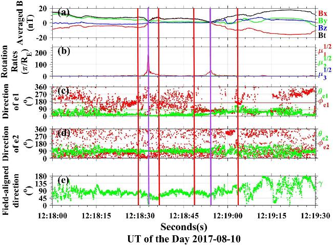
Figure 8. (a) Changes in magnetic field strength Bx, By, Bz, and Bt, (b) the maximum ${\mu }_{1}^{1/2}$, intermediate ${\mu }_{2}^{1/2}$, and minimum ${\mu }_{3}^{1/2}$ rotation rates of the magnetic field; (c) azimuth θe1 and φe1 of eigenvector e1; (d) azimuth θe2 and φe2 of eigenvector e2; (e) angle between current and magnetic field γ detected by the four MMS satellites from 12:18:00 to 12:19:30 on August 10, 2017. The red vertical lines represent the boundaries of the current sheets and purple vertical lines show the center of the current sheet. |
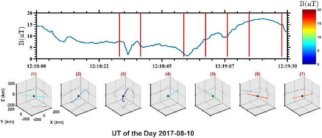
Figure 9. Schematic diagram of the three-dimensional topology of magnetic field lines in the early phase of a flux tube entanglement event during the UT period from 12:18:00 to 12:19:30 on August 10, 2017. |
To further analyze the FCS and its evolution, local quantitative and qualitative features of MFL topologies are determined by the geometrical invariants. Figure 10 shows the normalized geometrical invariants's signals with respect to time, (a) changes in magnetic field strength, (b) for Qn, (c) Rn, and (d) Dn. The subscript n means being normalized by time averaged current flux, i.e. ${Q}_{n}=Q/\left\langle j\right\rangle $, ${R}_{n}=R/{\left\langle j\right\rangle }^{3/2}$. It can be seen that, for most of the time, Qn and Rn are close to zero, implying that there are no characteristic structures measured by MMS. At about 12:18:32 UT, Qn appears with a negative peak whose value is about −0.001. Note that this negative peak corresponds to the transition between two different magnetic flux tubes. Associated Rn also shows a negative and positive peak and Dn presents an abrupt negative peak. These characteristics indicate that MMS encounters a magnetic structure. Figure 11 shows tracks of Qn and Rn, where the color bar from blue to red denotes the time from 12:10:00 UT to 12:19:30 UT on 2017-08-10. We can see that, during the transition region, (Rn, Qn) lies mostly in the Dn < 0 regime, which means that MMS mostly measured magnetic flux tubes like structures only. The close temporal correspondence between the abrupt changes in the magnetic field components and the extrema in Qn, Rn, and Dn suggests that these topological indicators effectively capture the localized and transient nature of the magnetic structures encountered by MMS. The confined duration of these signatures further implies that the associated current layers are spatially thin and dynamically evolving, as expected in an active reconnection environment in the magnetotail.
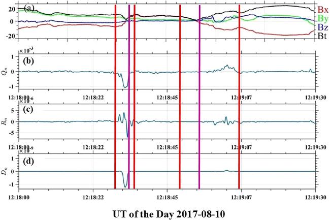
Figure 10. (a) Changes in magnetic field strength Bx, By, Bz, and Bt, normalized geometrical invariants signals with respect to time, (b) for Qn, (c) for Rn and (d) for Dn during the UT period from 12:18:00 to 12:19:30 on August 10, 2017. |
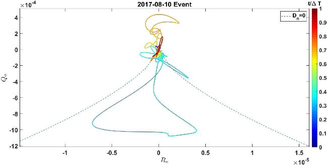
Figure 11. Tracks of Qn and Rn, where color bar from blue to red denotes the time from 12:18:00 to 12:19:30 on August 10, 2017. |
4.2. Second event
Figure 12 shows the traversal event of the current sheet on July 06, 2017, from 08:31:00 UT to 08:32:00 UT, which is similar to the current sheet in Event 1, but differs from the previous one in that the magnetic field component of the event at the center of the current sheet is By < 0. Figure 12(c) illustrates that the magnetic field component in the z-direction (Bz) remains very weak across the current sheet and approaches zero at the mid-point of the neutral current sheet. In contrast, figure 12(b) shows that the y-direction component (By) maintains a value close to −6.6 nT. Figure 13 illustrates the changes in various parameters during a specific time interval on July 06, 2017, from 08:31:00 UT to 08:32:00 UT. Figures 13(a) and (b) demonstrate that near the neutral sheet, the BM component of the magnetic field and the JM component of the current density exhibit minimal variation in the direction orthogonal to the current sheet, with both tending toward zero. Concurrently, the BM magnetic field component undergoes a polarity shift—transitioning from positive to negative or vice versa—while the magnitude of the current density increases markedly. Furthermore, figure 13(b) presents the spatial profile of the current density across the current sheet, indicating that the principal contributions to the total current density at the neutral sheet originate from its components aligned with both the L direction and the magnetic field orientation. The region delineated by the two red vertical lines corresponds to a well-defined current sheet crossing observed by MMS, with the purple line marking the location of the current sheet center. Within this interval, the magnetic field components exhibit systematic rotations and sign reversals, while the total magnetic field magnitude shows a localized reduction, consistent with the spacecraft traversing a thin magnetotail current sheet. Near the central plane of the sheet, enhanced gradients and fluctuations in the magnetic field components indicate intensified current density and proximity to the neutral plane. In parallel, the plasma parameters display modest but discernible variations, including localized enhancements in particle densities and pressures, reflecting plasma compression and energization within the current sheet environment. In contrast, outside the current-sheet interval, both magnetic field and plasma quantities remain comparatively stable, underscoring that the observed signatures are spatially confined to the current sheet structure. Collectively, these observations characterize a coherent and well-organized current sheet with a distinct central region, providing favorable conditions for current concentration and associated kinetic-scale processes.
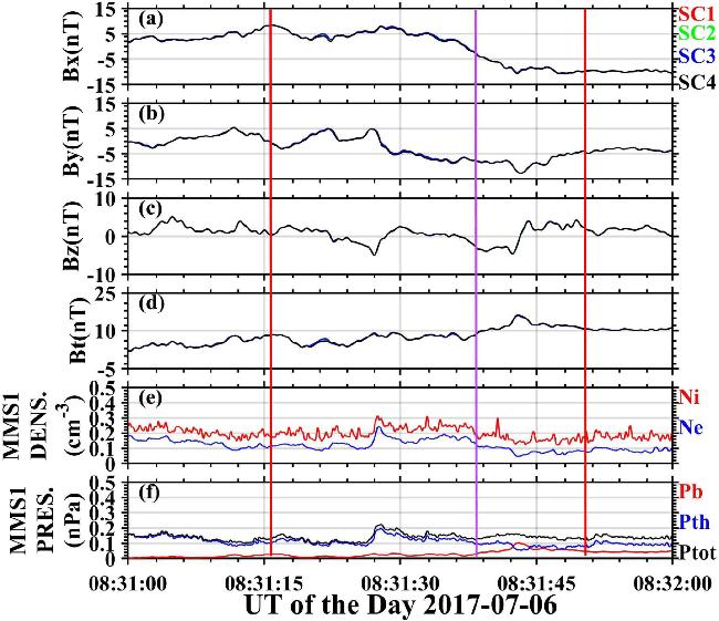
Figure 12. Changes in magnetic field strength (a) Bx, (b) By, (c) Bz, and (d) Bt, (e) electron ion density Ne, and Ni, (f) thermal pressure Pth, magnetic pressure Pb, and total pressure Pt detected by the four MMS satellites from 08:30:55 to 08:31:55 on July 06, 2017. The red vertical lines represent the boundaries of the current sheet and purple vertical line shows the center of the current sheet. |
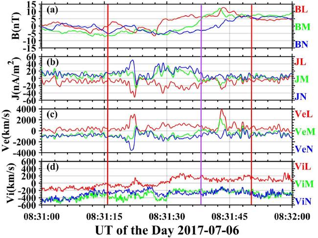
Figure 13. Changes in (a) magnetic field intensity BL, BM, and BN, (b) current density JL, JM, and JN, and (c) electronVeL, VeM, VeN, (d) ion velocities ViL, V${}_{{iM}}$, ViN of the magnetic field structure in the GSE coordinate system from 08:31:00 to 08:32:00 on July 06, 2017. The red vertical lines represent the boundaries of the current sheet and purple vertical line shows the center of the current sheet. |
Notably, the dominant current direction aligns inversely with the magnetic field, with the maximum current density surpassing 36 nA m2, indicating a remarkably strong current density. It appears that a very robust interaction occurs where the polarity reversal takes place. Examining figure 13(c) and observing the curve depicting changes in electron velocity, it is evident that as the satellite crosses the neutral sheet, there is a substantial boost in electron velocity, resulting in the observation of an ultra-Alfven electron flow. Specifically, the electron velocity reaches VeL = 1800 km s−1 in the L direction, roughly 2.3 times the Alfven speed (VA), and VeN = 800 km s−1 in the N direction, approximately equal to VA. Notably, VA, calculated at around 790 km s−1, serves as the Alfven speed. These findings strongly suggest that magnetic field reconnection has transpired at the near neutral sheet location, yielding an exceptionally rapid electron jet. When figure 13(d) is considered alongside this, it becomes evident that the electron's velocity significantly surpasses that of the ion, establishing the electrons as the primary carrier, with acceleration and inversion occurring along the M direction. The NMG algorithm is then utilized to determine the primary and secondary magnetic field gradients. Collectively, these observations characterize a well-organized, thin current sheet with a distinct central region, where intensified currents and decoupled electron–ion dynamics are evident, providing favorable conditions for kinetic-scale processes associated with magnetic reconnection.
As shown in figure 14(b), the magnetic field's curvature drops to zero at the neutral sheet. When the MMS satellite traverses the current sheet, this curvature reaches its minimum at the sheet's center. Moreover, figure 14(c) indicates that the helix angle remains approximately 90° throughout the neutral sheet and decreases to its lowest point at the center. This suggests that the field lines configuration of the sheet follows a helical, rather than a planar, path. Moreover, figure 14(b) shows that the curvature radius of the MFL is smaller than the Earth's radius (RE), indicating the presence of an extremely narrow current sheet. At the center, the radius of curvature reaches its minimum value of approximately Rc ≈ 0.16RE, or around ≈1024 km. The MFL curvature on the southern side of the current sheet initially directs northward, as shown in figure 14(b). As the satellite approaches the central region of the current sheet, both the MFL curvature and the orientation of the secondary normal vector exhibit significant variability. This behavior implies that within the neutral sheet, MFLs adopt a helical configuration. At the precise center of the neutral sheet, indicated by the purple vertical line, the secondary normal vector of the magnetic field is oriented nearly south, corresponding to a polar angle (θN) of 11.7°. As the MMS spacecraft continues its trajectory northward across the current sheet, the direction of curvature progressively shifts southward. These findings collectively suggest that the MFL undergoes a clockwise rotation about the northward-pointing normal vector of the current sheet, forming a left-handed helical structure. Additionally, the curvature attains its peak magnitude at the center of the neutral sheet and remains close to zero in surrounding regions. As shown in figure 14(d), the torsion exhibits its most pronounced variation in proximity to the neutral sheet, further supporting the interpretation of a spiral magnetic field configuration. These combined signatures demonstrate that the magnetic field geometry within the current sheet is highly structured and three-dimensional, with enhanced curvature and torsion concentrated near the sheet center, consistent with a dynamically evolving current layer that may facilitate localized magnetic reconnection and field-line deformation.
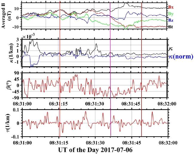
Figure 14. Variation curves of (a) magnetic field strength Bx, By, Bz, and Bt, (b) curvature (c) helix angle and (d) torsion of the magnetic field lines calculated by the NMG algorithm during the UT period from 08:31:00 to 08:32:00 on July 06, 2017. |
As the MMS satellite moves from the northern to the southern region of the current sheet (refer to figure 15), the polar angle (θB) of the magnetic field vector remains close to 90° [figure 15(b)]. Conversely, the azimuthal angle (φB) undergoes a rotation of approximately 180°, eventually stabilizing around φB ≈ 180°. This azimuthal variation is most significant within the central segment of the current sheet—demarcated by the two red vertical lines in figure 15—which is commonly identified as the neutral sheet. At the midpoint of this region, the magnetic field vector is characterized by a polar angle of roughly θB ≈ 190° and an azimuthal angle around φB ≈ 270°, which indicates the field is oriented toward the morning sector. Figure 16(c) further illustrates this substantial rotation of the magnetic field within the neutral sheet. Meanwhile, figure 16(c) reveals that the direction of this rotation, as represented by the principal eigenvector (e1), predominantly points northward, with a polar angle of ${\theta }_{{e}^{1}}=5.6^\circ $ at the center. Figures 16(e) and (f) illustrate a pronounced concentration of electric current within the thin neutral sheet, indicating that both the current density and the rotation of magnetic field vectors are primarily confined to this narrow region. As depicted in figure 16(e), the directions of the current and magnetic field are predominantly anti-parallel at the center of the neutral sheet, where the angle γ approaches approximately 170°. The local three-dimensional structure of the MFLs is visualized through a line-tracing technique, and their geometric arrangement at the neutral sheet is depicted in figure 17. The magnetic field orientation analysis further shows that the polar angle of the magnetic field vector remains close to 90°, indicating that the current sheet is aligned with the equatorial plane. In contrast, the azimuthal angle rotates by approximately 180° across the sheet, with the strongest rotation occurring within the neutral sheet. MRA confirms that this rotation is highly localized, with the principal rotation axis oriented nearly northward. At the sheet center, the electric current and magnetic field are almost antiparallel, with the angle between them approaching 170°, consistent with strong field-aligned current flow confined to the thin neutral sheet. MFL tracing confirms a distinct helical structure at the neutral sheet, in agreement with the gradient and rotation analyses.
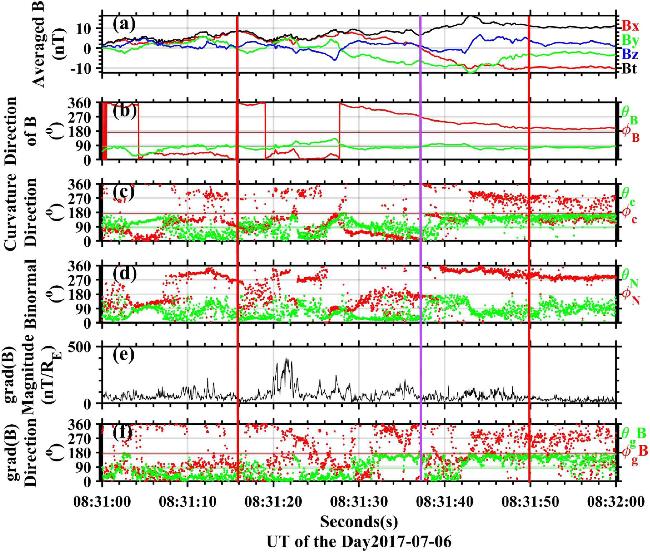
Figure 15. (a) Changes in magnetic field strength Bx, By, Bz, and Bt, (b) polar θB and azimuth φB angles of the magnetic field vector; (c) the azimuth sum of the curvature of the magnetic field lines θc and φc; (d) the azimuth θN and φN of the subnormal vector of the magnetic field lines; (e) first-order gradient of magnetic field strength; (f) the azimuth θgB and φgB of the first-order gradient of magnetic field strength detected by the four MMS satellites from 08:30:55 to 08:31:55 on July 06, 2017. The red vertical lines represent the boundaries of the current sheet and purple vertical line shows the center of the current sheet. |
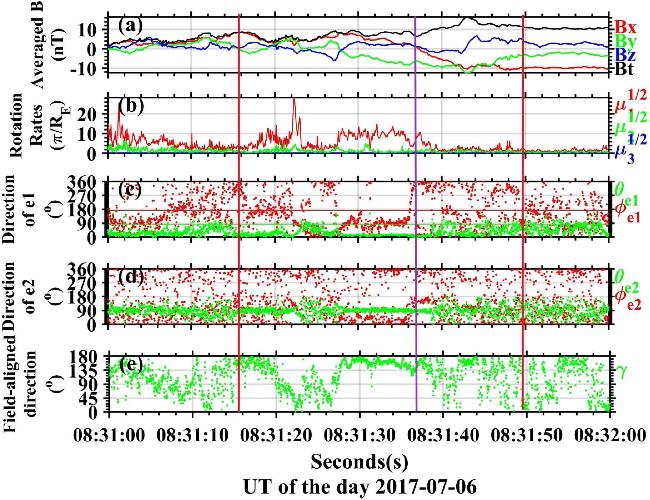
Figure 16. (a) Changes in magnetic field strength Bx, By, Bz, and Bt, (b) the maximum ${\mu }_{1}^{1/2}$, intermediate ${\mu }_{2}^{1/2}$, and minimum ${\mu }_{3}^{1/2}$ rotation rates of the magnetic field; (c) azimuth θe1 and φe1 of eigenvector e1; (d) azimuth θe2 and φe2 of eigenvector e2; (e) angle between current and magnetic field γ detected by the four MMS satellites from 08:30:55 to 08:31:55 on July 06, 2017. The red vertical lines represent the boundaries of the current sheet and purple vertical line shows the center of the current sheet. |
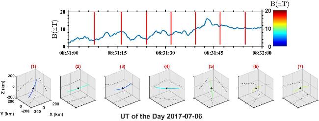
Figure 17. Schematic diagram of the three-dimensional topology of magnetic field lines in the early phase of a flux tube entanglement event during the UT period from 08:31:00 to 08:32:00 on July 06, 2017. |
Figure 18 displays the time variation of (a) magnetic field, (b) Qn, (c) Rn and (d) Dn. During most of the time, Qn and Rn are not close to zero, indicating that the magnetic field is not homogeneous, with obviously a change in the scale of MMS. Near the transition time when MMS passes from the neutral sheet, Qn and Rn obviously become smaller than zero, then become larger than zero. This means that the neutral sheet shows different magnetic structures. Associated Dn shows two large negative peaks near 08:31:22 UT and 08:31:32 UT. This implies that MMS first passes through a magnetic flux tube, then passes through the transition region. The time interval enclosed by the two red vertical lines corresponds to a well-defined current sheet crossing, with the purple line indicating the central plane of the sheet. Within this region, the averaged magnetic field components show pronounced and coherent variations, including systematic rotations and changes in magnitude, consistent with a traversal of a thin and structured current layer. The topological and geometric diagnostics exhibit clear enhancements inside the current sheet: the Q-criterion and the R- and D-parameters display intermittent but significant excursions, with the most prominent extrema occurring near the sheet center. These localized enhancements indicate increased magnetic field-line twisting, rotational deformation, and local compressibility within the current sheet, pointing to a departure from simple planar geometry. In contrast, outside the current-sheet interval, the diagnostic parameters remain near background levels, reflecting relatively smooth magnetic field topology in the surrounding plasma sheet. The concentration of strong topological signatures near the central plane suggests that the current sheet hosts localized, three-dimensional magnetic structuring and enhanced magnetic deformation, providing favorable conditions for the development of small-scale reconnection-related or turbulent features within the current layer. Figure 19 shows the tracks of Qn and Rn, where the color bar from blue to red denotes the time on 06 July 2017, from 08:31:00 UT to 08:32:00 UT. We can see that during the transition region, (Rn, Qn) go across mostly through Dn < 0, which means MMS confronted with magnetic flux tube mostly. Compared to the first event, we can observe mostly magnetic flux tube like structures in this event. This shows a weak magnetic field transition as compared to the first event because magnetic flux tubes are the weak candidates to carry magnetic field as compared to magnetic flux ropes. Also, this figure shows that during this type of event of FCS evolution, the magnetic flux rope plays the main role in reconnection.
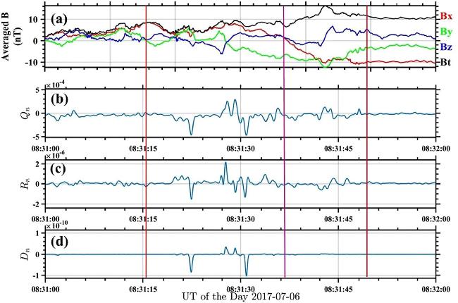
Figure 18. (a) Changes in magnetic field strength Bx, By, Bz, and Bt, normalized geometrical invariants signals with respect to time, (b) for Qn, (c) for Rn and (d) for Dn during the UT period from 08:31:00 to 08:32:00 on July 06, 2017. |
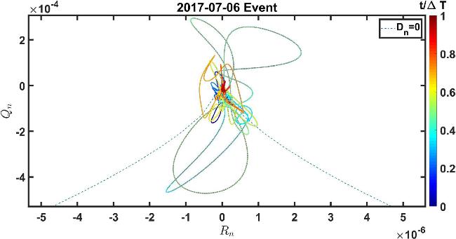


Figure 19. Tracks of Qn and Rn, where color bar from blue to red denotes the time from 08:31:00 to 08:32:00 on July 06, 2017. |
5. Conclusion
This study investigates the role of magnetic flux function and geometrical analysis of field line topology in magnetic reconnection events using an advanced multi-point approach, specifically the NMG algorithm and geometric invariant techniques. To understand the diffusion process responsible for magnetic reconnection in various magnetic flux topologies, equilibrium states were considered within a highly idealized two-dimensional magnetosphere. Several contour plots illustrate the analytical variations in Earth's magnetic field diffusion profile across different characteristic length scales. The analytical calculations suggest that quadratic magnetic gradient estimators, along with the overall geometry of MFLs, are effective in examining magnetic configurations and structures in space plasmas. This is especially true when using precise multi-point measurements in comparison with theoretical models. Furthermore, a parametric analysis of the current sheet is conducted, taking into account observational data in relation to the background magnetic field and variations in distance. At the beginning of the event, observations indicate that the y-component of the magnetic field (By) near the center of the current sheet measures approximately 2.03 nT, with the total magnetic field strength recorded at about 2.08 nT. This suggests the presence of a significant guide field concentrated within the sheet's core region. Additionally, a relatively minor Bz component, approximately 0.2 nT, is detected near the neutral sheet. The structure of this current sheet diverges from standard configurations due to the notably strong By component at the neutral line. Moreover, the BM component exhibits a reversal in polarity—from a positive-to-negative transition to a negative-to-positive one—accompanied by an enhanced current density. The dominant contributions to the total current density within the neutral sheet primarily arise from the M-direction and field-aligned components.
A notable feature is the strong current density, peaking above 170 nA m2, which runs counter to the magnetic field direction. This is coupled with a substantial increase in electron velocity, leading to the detection of an ultra-Alfvenic electron flow. Specifically, the electron velocity in the M-direction reaches 6000 km s−1, approximately 7.6 times the Alfven speed, while in the L-direction, it is 5000 km s−1, about 6.3 times the Alfven speed. These findings indicate that magnetic reconnection is occurring near the neutral sheet, producing a highly accelerated electron jet. The electron velocity far exceeds that of ions, confirming electrons as the primary charge carriers with their movement and acceleration primarily along the M-direction. During the MMS satellite's first crossing of the current sheet, the neutral sheet's center exhibited maximum curvature, measuring approximately κ ≈ 0.02 km−1, with a corresponding curvature radius of Rc ≈ 0.01RE ≈ 50 km, consistent with prior research. As the satellite nears the central region, the MFLs exhibit a shift in curvature, indicating a helical rather than flat configuration. Subsequent analysis indicates that the magnetic field within the neutral sheet undergoes a clockwise rotation, resulting in a left-handed helical configuration. The curvature is at its maximum at the neutral sheet's center but approaches zero at other locations. The helix angle fluctuates around 45° in the neutral sheet, reaching its lowest value in the center. Additionally, torsion exhibits maximum variation at the neutral sheet's core and minimal variation in surrounding regions. This indicates that the magnetic field within the current sheet assumes a helical structure, rather than being confined to a planar alignment. At its center, the magnetic field vector is characterized by a polar angle of θB = 95° and an azimuthal angle of φB = 79°. During the transition region, MMS primarily detected magnetic flux tube-like structures, as (Rn, Qn) mostly fell within the Dn < 0 range.
During the second event, the z-component of the magnetic field (Bz) consistently remains low throughout the current sheet, approaching negligible values near the center of the neutral sheet. Concurrently, the y-component (By) maintains an approximate value of −6.6 nT. In the region surrounding the neutral sheet, both the magnetic field magnitude (BM) and the current density (JM) exhibit minimal variation along the direction perpendicular to the current sheet, remaining largely stable and close to zero. Meanwhile, BM undergoes a polarity reversal (positive to negative or vice versa), which coincides with a notable increase in current density. The primary current direction opposes the magnetic field, with a peak current density exceeding 36 nA m2, signifying a strong current flow. A significant rise in electron velocity leads to the emergence of an ultra-Alfvénic electron flow. Specifically, electron velocity reaches VeL = 1800 km s−1 along the L direction, about 2.3 times the Alfvén speed (VA), and VeN = 800 km s−1 along the N direction, nearly equal to VA. As the MMS spacecraft crosses the current sheet, a pronounced reduction in magnetic field curvature is observed near the central neutral region. Examination of the helix angle profile reveals that within the neutral sheet, the mean helix angle tends toward 90°, with the lowest value occurring precisely at the sheet's midpoint. This pattern indicates that the magnetic field structure diverges from a planar geometry, instead exhibiting a helical configuration. At the core of the current sheet, the minimum radius of curvature is estimated to be approximately Rc ≈ 0.16RE, corresponding to roughly 1024 kilometers. Recurrent changes in the curvature direction and the orientation of the subnormal vector further support the interpretation that the MFLs follow a spiral path within the neutral region. Variations in the helix angle around this region provide additional confirmation of the helical nature of the field. The magnetic field vector's polar angle (θB) remains close to 90°, while the azimuthal angle (φB) rotates around 180°, eventually stabilizing near that value. Most of these azimuthal variations are observed within the neutral sheet. At its center, θB and φB reach approximately 190° and 270°, respectively, indicating the magnetic field vector is oriented toward the morning sector. Compared with the first event, this event primarily exhibits magnetic flux tube-like structures. These structures indicate a weaker magnetic field transition than the first event, as magnetic flux tubes are less effective in carrying magnetic fields than magnetic flux ropes. In summary, both current sheet crossings demonstrate that magnetic reconnection in the magnetotail can generate thin current sheets with strong electron-scale activity and three-dimensional helical magnetic structures. However, the first event corresponds to a weaker reconnection regime dominated by flux-tube-like structures and reduced current and particle acceleration, whereas the second event represents a more intense and dynamically active reconnection scenario dominated by flux rope formation and ultra-Alfvénic electron jets. Together, these observations highlight the variability of magnetotail reconnection and underscore the role of guide-field polarity, current intensity, and magnetic topology in controlling current sheet evolution and energy conversion.