Reaction–diffusion infectious disease models are widely used to describe the spatial distribution of infected individuals. In this study, we construct network-based reaction–diffusion models that incorporate both higher-order interactions and advection mechanisms, formulated on a triangular lattice torus network. This idealized structure is adopted to facilitate explicit derivation and linear stability analysis of the theoretical conditions for Turing instability—analyses that would be considerably more challenging in complex heterogeneous geometries. To address the computational challenge of generating higher-order node Laplacian matrices in large-scale networks, we develop a dimensionality reduction strategy using graph-structured edge Laplacians. The theoretical analysis reveals how higher-order interactions and advection jointly influence the onset of Turing patterns. Furthermore, model fitting to real epidemic data—using a mobility network constructed from 2020 inter-prefectural commuting flows across Japan's 47 prefectures—shows that incorporating higher-order interactions results in better fitting performance compared to conventional models.
Wenlong Zhang, Xuerui Zhu, Linhe Zhu. Spatiotemporal heterogeneity of a network epidemic model with higher-order interactions and advection mechanisms[J]. Communications in Theoretical Physics, 2026, 78(6): 065602. DOI: 10.1088/1572-9494/ae4c74
1. Introduction
Infectious diseases have always been a focus of global public health security. In recent years, outbreaks of emerging infectious diseases (e.g. HIN1 influenza A) and the drive for population mobility have exacerbated the complexity and uncertainty facing infectious disease prevention and control. The world's low-fertility, aging countries with rising proportions of patients with chronic diseases have exacerbated the healthcare burden and socioeconomic impact. In this context, there is an urgent need for infectious disease research to think from a multidisciplinary cross-cutting perspective: analyzing pathogen adaptations at the biomathematical level, using big data to predict epidemic persistence cycles at the computational mathematical level, and so on. In addition, optimizing public health policies and improving information drivers also provide new ideas for reducing the threat of infectious diseases.
Ordinary differential equations in mathematics, a fundamental tool for dynamical systems [1–3], have deepened their modeling capabilities in the field of infectious disease dynamics through the development of susceptible-infected-recovered (SIR) models [4]. Existing studies have enriched the traditional compartmental framework by introducing mechanisms such as the Allee effect [5], differential mortality weights [6], and nonlinear recovery rates [7]. These analyses extend the traditional framework, while this study combines the core ideas of the literature [6–8]. Other well-recognized features include time-delay effects (e.g. pathogen latency, delayed prevention and control) [9–12]. While our work does not explicitly incorporate time-delay mechanisms, it focuses on improving spatial modeling by constructing a multi-region diffusion–advection framework. In response to the limitations of classical compartmental models in capturing spatio-temporal dynamics, researchers have incorporated spatial variables into epidemic models to enable kinetic analysis [13–15]. For example, Kunz [14] revealed the mechanism of biological pattern formation driven by spatial heterogeneity through coupled diffusion-reaction-convergence, which had broken through the assumption of homogenization under the traditional pattern. Building upon this, network-based epidemic models have been developed to further address the limitations of conventional spatio-temporal frameworks [16–24]. Satorras [16] introduced a networked SIR model based on the Laplace matrix and had revealed the moderating role of the social topology in the propagation dynamics of infectious diseases. Yu [17] further verified the synergistic relationship between network topology and cross-diffusion coefficient on system stability regulation by using the 2SIR model. In another aspect of model development, the advection mechanism has been widely used in various disciplines [25–30]. Wu [29] investigated the long-term dynamics of a cyclic response-advection-dispersal schistosomiasis model, emphasizing the combined effects of advection, seasonality, and spatial heterogeneity on disease transmission. Yang [30] established a network reaction–diffusion model with directional migration term, which revealed the mechanism of pattern formation based on advection effect.
In fact, despite the simplicity of the form of traditional complex network models and their success in capturing the fundamental interactions (pairwise interactions) of complex systems, their fundamental limitation of reducing complex phenomena to a linear superposition of pairwise interactions between nodes has been demonstrated by a large number of studies. Although complex networks effectively model pairwise interactions via edges, numerous socially relevant transmission scenarios (such as shared workplaces and social gatherings) inherently involve synchronous interactions among three or more individuals. In such settings, infection risks stem from the very act of group cohabitation within shared spaces, a characteristic more accurately captured by 2-simplicial complexes than by independent pairwise interactions. The propagation dynamics of real social systems are intrinsically inseparable from higher-order interactions, which has focused the academic community on the construction of higher-order networks [31–38]. Song [31] closed higher-order structures based on dynamic equations break away from traditional node-centered networks, and proposed a higher-order propagation mechanism featuring hyperedge weights. Further theoretical breakthroughs are reflected in the regulation mechanism of the uniformity of the Turing pattern. Through the regulation of the strength of the higher-order interactions in the simple complex form, Luo [35] found that an increase in the strength drived the distribution of the density of infections to homogenization, which was conducive to optimizing the rational allocation of resources during an outbreak of an infectious disease. Building on recent advances in simplicial complex-based modeling—particularly Muolo [36]'s finding that higher-order structures can reshape the conditions for Turing instability—we propose a networked epidemic model that integrates both higher-order diffusion and directional advection. In this framework, higher-order diffusion emerges from three-body interactions defined on a triangular lattice, capturing the coordinated movement among region triplets. Meanwhile, the advection term reflects directional flows influenced by environmental or infrastructural factors. Although these mechanisms have been investigated separately in epidemic dynamics [30, 32], their combined effect on spatiotemporal pattern formation remains largely unexplored. To address this gap and enable scalable simulations, we design a graph-structured dimensionality reduction strategy. This method significantly reduces computational complexity while preserving essential higher-order topological features.
The rest of the paper is organized as follows: In section 2, we develop a higher-order network-based infectious disease model. In section 3, we study the necessary conditions for lower-order diffusion, higher-order diffusion and advection to cause Turing instability. In section 4, we focus on the application of our model to real-world data and networks. Using empirical inter-prefectural mobility data for Japan's 47 prefectures, we construct a directed, weighted commuting network and fit the full heterogeneous-parameter PDE system simultaneously to all prefectures. The fitting is performed with physics-informed neural networks (PINNs) [39, 40], enabling the integration of observational data with the governing dynamical equations. We then assess the role of higher-order spatial interactions in this realistic setting by comparing fits with and without higher-order terms, quantifying the changes in RMSE across prefectures. Finally, we present the conclusions of this paper in section 5.
2. Modeling
In the transmission of infectious diseases, we divide the population into three parts.
•
•S(Susceptible individual). Target groups for the transmission of infectious diseases that are not infected but are at risk of being infected.
•
•I (Infected individual). Groups of people who carry pathogens, contract diseases and spread them.
•
•R (Recovered individual). Groups of people who have successfully cleared pathogens, recovered from infectious diseases and gained immunity.
In the framework of the classical SIR model, there are three states of nodes in space: susceptible individual, infected individual and recovered individual. We assume that the recovered individual is no longer involved in subsequent propagation, i.e. it has no influence on the dynamics of the S − I subsystem. We then construct an networked infectious disease model with higher-order interactions on a complex network space $\left({\rm{\Omega }}=1,\cdots \,,N\right)$ with discrete nodes. The model reflects the change in node population density over time through an ordinary differential equation with the following expression:
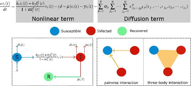
We now give the biological interpretation of parameters in model (1). A is the population replenishment rate, d is the natural mortality rate, μ is the disease-induced mortality rate, and γ is the recovery rate. The model describes the following dynamic behavioral or transformational relationships between different populations in an infectious disease transmission setting:
▶Disease transmissibility ($\frac{{k}_{1}{I}_{i}+{k}_{2}{I}_{i}^{2}}{1+\alpha {I}_{i}^{2}}{S}_{i}$). Describe the number of new infections per unit of time in the susceptible individuals.
▶Growth rate of disease infectivity (k1Ii). Baseline transmission.
▶Infectivity of the disease (${k}_{2}{I}_{i}^{2}$). Enhanced spread at high infected density.
In figure 1, we take the equation for the infected individuals as an example. The population state transition network on the left side demonstrates the coupling mechanism within the nonlinear term, where arrows pointing in indicate an increase in that state and pointing out indicates a decrease. The right side visually portrays how the diffusion term acts, i.e. pairwise interactions through 1-simplexes (links), and three-body interactions through 2-simplexes (triangles). In order to ensure the rationality of the model parameters, based on the physical or realistic significance of the actual application scenarios, all parameters are set to be non-negative real numbers.
Figure 1. Schematic diagram of the SIR higher-order infection epidemic model with birth, death, and recovery.
As described in [36], σp stands for the coupling strength, we assume that the maximum interaction that exists is $\left(P+1\right)$-body interaction, so p belongs to {1, ⋯ , P}. The (p + 1)-body interactions are denoted by the p-th adjacency tensor Ap, which means that (p + 1)-body interactions between nodes i, j1, ⋯ , jp is given by ${A}_{i{j}_{1}\cdots {j}_{p}}^{p}=1$. In order to construct higher-order coupling terms with diffusion-like properties, we assume that there exists a function hp( · ) for each dimension p such that the coupling function ${g}_{p}({S}_{{j}_{1}},\cdots \,,{S}_{{j}_{p}})$ can be written in the form of a state difference:
This construction method is not universally applicable. It has, however, been used as a reasonable modeling assumption in studies such as higher-order coupled oscillator networks (see [31]) and reaction–diffusion networks (see [36]). Its advantages include: ensuring that the coupling terms are zero in the steady state, offering a clear physical analogy with diffusion, and facilitating stability analysis and modal expansion. We adopt this assumption here to enable tractable analysis. Mathematically, the definition of gp when xi = xj ensures that the coupling vanishes when all nodes are in the same state
In order to focus on higher-order interactions, we do not consider the cross-diffusion term. This simplification allows us to focus only on pairwise (first-order) interactions and three-body (second-order) interactions without loss of generality. At the same time, we define $F({S}_{i},{I}_{i})\triangleq A-{\rm{d}}{S}_{i}-\frac{{k}_{1}{I}_{i}+{k}_{2}{I}_{i}^{2}}{1+\alpha {I}_{i}^{2}}{S}_{i}$ and $G({S}_{i},{I}_{i})\triangleq \frac{{k}_{1}{I}_{i}+{k}_{2}{I}_{i}^{2}}{1+\alpha {I}_{i}^{2}}{S}_{i}-(d+\mu ){I}_{i}-\gamma {I}_{i}$, we have
As pointed out in the literature [41], if higher-order interactions are linear, then they are essentially superpositions of pairwise interactions. For ease of analysis, we focus on the quadratic form as a natural extension of linearity. Specifically, all interactions considered in this study are quadratic. The specific functional forms are
This study starts from the stability analysis of an isolated system, where only local reactions are considered and interactions between units are not taken into account. Under this assumption, the equilibrium point of the model (3) must be satisfied $F({S}_{i}^{* },{I}_{i}^{* })=0$ and $G({S}_{i}^{* },{I}_{i}^{* })=0$. We denote the equilibrium point $\left({S}_{1}^{* },{I}_{1}^{* },{S}_{2}^{* },{I}_{2}^{* },\cdots \,,{S}_{N}^{* },{I}_{N}^{* }\right)$ as $\left({S}_{* },{I}_{* },{S}_{* },{I}_{* },\cdots \,,{S}_{* },{I}_{* }\right)$.
where $a=\left({k}_{2}+d\alpha \right)$$\left(d+\mu +\gamma \right)$, $b={k}_{1}\left(d+\mu +\gamma \right)\,-A{k}_{2}$, $c=d\left(d+\mu +\gamma \right)-A{k}_{1}$. To ensure the relevance of the solution, S* > 0 and I* > 0, the necessary condition for the existence of a positive equilibrium point, needs to be satisfied. We first give the necessary condition for I* > 0
This contradicts the fundamental assumption that all parameters remain positive. Consequently, the inequality ${I}_{* }\lt \frac{A}{d+\mu +\gamma }$ must hold universally, implying that whenever equation (4) is satisfied, ${S}_{* }=\frac{A-\left(d+\mu +\gamma \right){I}_{* }}{d}\gt 0$ necessarily follows. To analyze the stability of model (3), we first compute the Jacobian matrix J0 at the equilibrium point (S*, I*, S*, I*, ⋯ , S*, I*) and subsequently derive its characteristic polynomial. The model (3) can be decomposed into N identical 2 subsystems, so that the overall characteristic equation of the full system takes the following form,
To ensure that the model (3) remains stable in the absence of disturbances, all characteristic roots must have negative real parts. A necessary condition for this stability is that ${\rm{tr}}({J}^{0})\lt 0$ and ${\rm{\det }}({J}^{0})\gt 0$. Based on this, the necessary condition for the onset of a Turing bifurcation is given by
3.2. Turing instability induced by pairwise interaction in model (3)
To determine the necessary conditions for Turing instability induced by pairwise interaction, the parameter σ2 in the model (3) is set to zero, and a Taylor expansion is carried out around the equilibrium point (S*, I*, S*, I*, ⋯ , S*, I*). Then we retain the linear term in order to obtain the following linearized system
The first-order Laplacian matrix L1 is defined as ${L}^{1}={\left({L}_{ij}^{1}\right)}_{N\times N}={A}^{1}-D$, where D = diag{k1, ⋯ , kN} is the degree matrix, ki represents the order of node i and A1 is a special adjacency tensor, which we also call the adjacency matrix. For an n-th nonzero eigenvalue Λn, the corresponding set of orthogonal eigenvectors is ${{\rm{\Phi }}}_{n}={\left({{\rm{\Phi }}}_{n}^{1},\cdots \,,{{\rm{\Phi }}}_{n}^{N}\right)}^{{\bf{T}}}$. The eigenvector associated with the zero eigenvalue is the all-ones vector Φ0 = (1, ⋯ , 1)T.
To express model (7) in a compact form, we introduce a perturbation vector $\zeta ={\left(\delta {S}_{1},\delta {I}_{1},\cdots \,,\delta {S}_{N},\delta {I}_{N}\right)}^{{\bf{T}}}$ and the following equation is obtained that
where ${J}_{{H}_{1}}=\left|\begin{array}{ll}2{S}_{* }{D}_{1}^{S} & 0\\ 0 & 2{I}_{* }{D}_{1}^{I}\end{array}\right|$, and ⨂ denotes the Kronecker product, which has a wide range of applications in higher-order networks. Then we project model (8) onto the eigenspace of L1:
the result of our projection is $\left(\begin{array}{c}\delta {\hat{S}}_{n}\\ \delta {\hat{I}}_{n}\end{array}\right)={\sum }_{i=1}^{N}\left(\begin{array}{c}\delta {S}_{i}{{\rm{\Phi }}}_{n}^{i}\\ \delta {I}_{i}{{\rm{\Phi }}}_{n}^{i}\end{array}\right)$. Subsequently, the terms $\delta {\hat{S}}_{n}$ and $\delta {\hat{I}}_{n}$ in model (9) is expanded in Fourier space, i.e. $\left(\begin{array}{c}\delta {\hat{S}}_{n}\\ \delta {\hat{I}}_{n}\end{array}\right)={\sum }_{k=1}^{N}\left(\begin{array}{c}{c}_{k}^{1}\\ {c}_{k}^{2}\end{array}\right){{\rm{e}}}^{{\lambda }_{k}^{p}t+{\rm{i}}kx}$, and we have
To make sure the existence of an eigenroots with a positive real part, it is necessary that at least one of ${\rm{tr}}({J}_{k}^{1})\lt 0$ and ${\rm{\det }}({J}_{k}^{1})\gt 0$ is not true. Given that ${\rm{tr}}({J}_{{H}_{1}})=2({S}_{* }{D}_{1}^{S}+{I}_{* }{D}_{1}^{I})\gt 0$, we can conclude that ${\rm{tr}}({J}_{k}^{1})\lt {\rm{tr}}({J}^{0})\lt 0$. Thus the necessary conditions for low-order diffusion to induce Turing instability is ${\rm{\det }}({J}_{k}^{1})\lt 0$, i.e.
3.3. Turing instability induced by higher-order interaction in model (3)
To study the necessary conditions for Turing instability induced by higher-order interaction, we perform a Taylor expansion of model (3) around the equilibrium point $\left({S}_{* },{I}_{* },{S}_{* },{I}_{* },\cdots \,,{S}_{* },{I}_{* }\right)$ and retain up to the linear term to obtain a linearized system as follows
If i ≠ j, ${\widetilde{L}}_{ij}^{2}$ denotes the number of 2-simplices formed by edges i and j. Similar to part B of this section, we write model (12) in a compact form by introducing a perturbation vector ζ,
where ${J}_{{H}_{2}}=\left|\begin{array}{ll}2{S}_{* }{D}_{2}^{S} & 0\\ 0 & 2{I}_{* }{D}_{2}^{I}\end{array}\right|$. We note that in model (13), L1 and ${\widetilde{L}}^{2}$ cannot generally be diagonalized simultaneously. That is, it is not possible to project this 2N × 2N system into the same feature space simultaneously. To address this limitation, we will proceed to analyze a specific coupling topology: the reqular topology.
In regular topologies with uniform structure, such as triangular lattice networks with periodic boundary conditions, the higher-order Laplacian matrices (e.g. second-order generalized Laplacians) can often be expressed as scaled versions of first-order Laplacians. This algebraic regularity allows model (13), originally defined on a 2N × 2N system, to be projected into a common eigenspace and decomposed into N independent 2 × 2 subsystems, greatly simplifying the analytical complexity.
Inspired by the principles of structural regularity and spectral clarity, we adopt a non-weighted, undirected triangular lattice on a toroidal surface as the underlying topology for our model. While simplified, this regular simplicial structure retains key geometric features relevant to higher-order diffusion. Conceptually, it echoes the analytical tractability demonstrated by the Weighted Triangulated Torus introduced by Wang [33], but deliberately omits the weighted and directional components to focus on the core mechanisms of pattern formation under higher-order interactions. This idealized setting enables clearer interpretation of spatial modes while acknowledging the abstraction from real-world complexity.
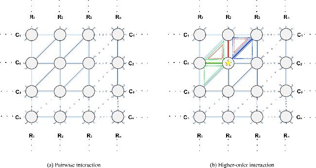
In figure 2(a), the triangular lattice torus network's diffusion layer is characterized by six principal connection directions for each node (Ri, Cj), which are Vertical Up: (Ri, Cj) → (Ri, Cj−1), Vertical Down: (Ri, Cj) → (Ri, Cj+1), Horizontal Left: (Ri, Cj) → (Ri−1, Cj), Horizontal Right: (Ri, Cj) → (Ri+1, Cj), Diagonal Southwest: (Ri, Cj) → (Ri−1, Cj+1), Diagonal Northeast: (Ri, Cj) → (Ri+1, Cj−1). Boundary nodes follow a periodic offset connection rule to maintain the torus topology. Let us take the first row as an example: Node (R1, C1) connects to (RN, C2) via diagonal northeast, Node (R1, C2) connects to (RN, C3). Other boundary nodes and so on. In figure 2(b), the specific pattern of three-body interactions in the triangular lattice network can be clearly presented. Now, taking the node labeled with a yellow pentagram as an example, only the participation of this node in three-body interactions with neighboring nodes vertically upward (red line), horizontally to the left (green line), and diagonally to the northeast (blue line) is presented.
For this triangular lattice torus network, each node participates in the formation of six 1-simplices, and each 1-simplice participates in the formation of two 2-simplices. We have
The eigenvalues of the first-order Laplacian matrix of the aforementioned triangular lattice torus network are obtained through mathematical methods (Appendix),
Based on the relationship of ${\widetilde{L}}^{2}=2{L}^{1}$, the eigenvalues of the second-order generalized Laplacian matrix can be obtained. Meanwhile, model (13) takes the following form:
Given that ${\rm{tr}}({J}_{{H}_{2}})=2({S}_{* }{D}_{2}^{S}+{I}_{* }{D}_{2}^{I})\gt 0$, we can conclude that ${\rm{tr}}({J}_{k}^{2})\lt {\rm{tr}}({J}^{0})\lt 0$. Thus the necessary conditions for higher-order diffusion to induce Turing instability is ${\rm{\det }}({J}_{k}^{2})\lt 0$, i.e.
3.4. Turing instability induced by advection mechanisms in model (3)
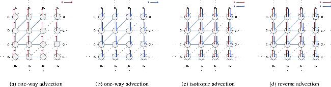
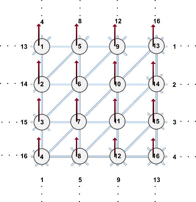
In figure 3, we show four advection mechanisms. In the structures shown in figures 3(a) and (b), within the stratosphere, each node has an efferent and incoming degree of 1, and each node points directly downward to a node in the same column. Similar to the connectivity pattern in the diffusion layer, the nodes in the last row point to the nodes in the first row of the same column. We define such a network as a triangular lattice torus network with one-way advection. In figures 3(c) and (d), there are two directional migration paths in the stratosphere. The directed migration paths for susceptible individuals and infected individuals may be the same or opposite, taking into account the effect of factors such as policy and information drivers. These two networks are referred to as triangular lattice torus networks of isotropic advection and reverse advection, respectively. Mathematically, the eigenvalues of the upward and downward advection matrices in figure 3(d) are ${\zeta }_{j}^{u}$ and ${\zeta }_{j}^{d}$ (Appendix),
As described in [30], the matrix $M={({m}_{ij})}_{N\times N}$ and the matrix $N={({n}_{ij})}_{N\times N}$ represent the Laplacian matrices of the directed advection networks corresponding to susceptible individuals and infected individuals, respectively. In addition, the parameters d1 and d2 are used to describe the advection strength that satisfies the conditions d1 ≥ 0 and d2 ≥ 0.
Figure 3. Advection methods in the triangular lattice torus network.
Let us perform a Taylor expansion of model (16) around the equilibrium point (S*, I*, S*, I*, ⋯ , S*, I*) and only keep the linear terms. We obtain a linearized system as follows
In the following text, we denote ${M}^{S}\triangleq 2{S}_{* }{\sigma }_{1}{D}_{1}^{S}{L}^{1}\,+2{S}_{* }{\sigma }_{2}{D}_{2}^{S}{\widetilde{L}}^{2}+{d}_{1}M$ and ${N}^{I}\triangleq 2{I}_{* }{\sigma }_{1}{D}_{1}^{I}{L}^{1}+2{I}_{* }{\sigma }_{2}{D}_{2}^{I}{\widetilde{L}}^{2}\,+{d}_{2}N$. To facilitate the analysis, we focus on a special case where MS can be diagonalized and MS = cNI, c ≠ 0. Under this condition, the initial 2N × 2N system can be projected into a common eigenspace and further decomposed into N 2 × 2 subsystems, thereby significantly reducing the overall analytical complexity.
We denote the eigenvalues of MS and NI by θ1, ⋯ , θN and ω1, ⋯ , ωN respectively. Furthermore, for all n ∈ Ω, the corresponding eigenvectors Φn of θn and ωn are identical and form an orthonormal basis. Each eigenvalue can be expressed as ${\theta }_{n}={a}_{n}^{S}+{\rm{i}}{b}_{n}^{S}$ and ${\omega }_{n}={a}_{n}^{I}+{\rm{i}}{b}_{n}^{I}$ for any n ∈ Ω. By the properties of the advection matrix, it follows that ${a}_{n}^{S}\leqslant 0$ and ${a}_{n}^{I}\leqslant 0$.
Similar to part C of this section, the system is projected onto the eigenspace of MS, and the perturbation is expanded in the Fourier space,
To ensure that equation (19) admits at least one root with a positive real part, we assume that the mth eigenvalue satisfies this condition. Let ${\lambda }_{(m,1)}^{a}={x}_{1}+{\rm{i}}{y}_{1}$ and ${\lambda }_{(m,2)}^{a}={x}_{2}+{\rm{i}}{y}_{2}$ denote the two corresponding roots. According to the Vieta formula in the complex domain,
Given that ${\rm{tr}}({J}^{0})\lt 0$, ${a}_{m}^{S}\lt 0$ and ${a}_{m}^{I}\lt 0$, we can conclude that $\mathrm{Re}\left({\lambda }_{(m,1)}^{a}+{\lambda }_{(m,2)}^{a}\right)\lt 0$. Thus, the necessary condition for the existence of the positive real part of the eigenvalue is
This situation differs from the necessary condition $\det ({J}_{k}^{2})\lt 0$ presented in part C of this section.
4. Numerical simulation
In this section, we perform numerical simulations of the theoretical part by using the forward Euler method. The network system is constructed by discretizing the time and space dimensions, where the space step Δx = 1 and the time step Δt = 0.01. The reliability of the theoretical part is verified by numerical simulation of the system by using the Neumann boundary on the region T × Ω. The initial condition is set as a small perturbation near the equilibrium state $\left({S}_{* },{I}_{* },{S}_{* },{I}_{* },\cdots \,,{S}_{* },{I}_{* }\right)$, which is manifested as
In numerical simulations of higher-order interactions, it is challenging to construct three-dimensional second-order Laplace matrices L2 when the number of nodes is high. Even with sparse matrix storage, the construction process is still significantly problematic. To this end, we propose a strategy for dimensionality reduction based on graph structure: as shown in figure 2(b), each edge (1-simplexe) ij belongs to two triangles (2-simplexes) ijk1 and ijk2. By this topological property, the double summation term ${\sum }_{j=1}^{N}{\sum }_{k=1}^{N}{A}_{ijk}^{2}\left({S}_{j}{S}_{k}-{S}_{i}^{2}\right)$ in model (3) can be simplified. Let us first consider the case where i ≠ j ≠ k,
In this way we downscale the three-dimensional second-order Laplacian matrix L2 into a two-dimensional second-order generalized Laplacian matrix ${\widetilde{L}}^{2}$. It is worth noting that although in the triangular lattice torus network we have ${\widetilde{L}}^{2}=2{L}^{1}$, the expression forms of pairwise interactions and higher-order interactions are structurally different. The pairwise term typically involves only self-coupling components such as ${\sum }_{j=1}^{N}{L}_{ij}^{1}{\left({S}_{j}\right)}^{2}$, whereas the higher-order term includes cross-node couplings like ${\sum }_{j=1}^{N}{\widetilde{L}}_{ij}^{2}{S}_{j}\frac{\left({S}_{{k}_{1}}+{S}_{{k}_{2}}\right)}{2}$, and so on. These cross terms represent collaborative effects among neighboring nodes, which cannot be captured by simple pairwise diffusion. In particular, terms like ${\sum }_{j=1}^{N}{\widetilde{L}}_{ij}^{2}{S}_{j}\frac{\left({S}_{{k}_{1}}+{S}_{{k}_{2}}\right)}{2}$ in the higher-order interactions contribute to a different mechanism of influence propagation. Therefore, even if the resulting Laplacian matrices share a scaling relationship, the functional roles of these interaction types in the dynamics are distinct, reflecting not just magnitude but also qualitative differences in the coupling structure.
In order to highlight the higher-order interactions, only a small number of typical low-order interaction scenarios are selected as controls for the subsequent simulations in this section. All objects plotted in this section are infected individuals. Unless otherwise specified, the color swatches represent the magnitude of the density of infected individuals.
4.1. Influence of higher-order interactions
To investigate the effect of higher-order interactions on Turing instability, we first focus on analyzing their effect on the eigenvalues of the model.
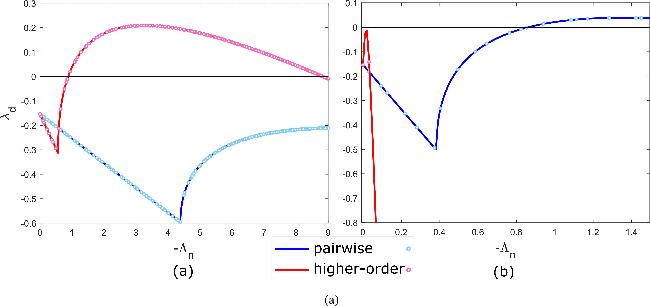
In figure 4, the parameters are fixed as A = 0.8, d = 0.12, μ = 0.02, γ = 0.6, α = 0.01, k1 = 0.07, k2 = 0.9, and ${D}_{1}^{S}={D}_{2}^{S}=1$. Here, λd denotes the maximum real part of the eigenvalues in equations (10) and (14), i.e. ${\lambda }_{d}=\max \mathrm{Re}({\lambda }_{i})$ (i = 1, 2, functions of Λn), known as the dispersion relation. A positive λd satisfies the necessary condition for Turing instability. The horizontal axis represents the eigenvalues of the first-order Laplacian L1: light blue dots show pairwise interactions, while light red dots include three-body interactions. Higher-order interactions can either promote or suppress Turing patterns. In figure 4(a) (${D}_{1}^{I}=0.2$, ${D}_{2}^{I}=0.1$, σ1 = σ2 = 0.1), they induce instability; in figure 4(b) (${D}_{1}^{I}=0.1$, ${D}_{2}^{I}=1$, σ1 = σ2 = 10), they suppress it. Since Λn is discrete, the results are interpolated into continuous curves for clarity.
Figure 4. Impact of higher-order interactions on λd.
Next, let us explore the effect of higher-order interactions on Turing patterns formation. Here, we fix the parameters: A = 0.28, d = 0.12, μ = 0.02, γ = 0.072, α = 0.01, k1 = 0.009, k2 = 0.296, ${D}_{1}^{S}={D}_{2}^{S}=1$, ${D}_{1}^{I}={D}_{2}^{I}=0.1$ and σ1 = 1. It can be observed that the density of infected individuals under this set of parameters shows fewer low-density areas (see figures 5–7).
Figure 7. Impact of higher-order interactions on Turing patterns formation at time 1000.
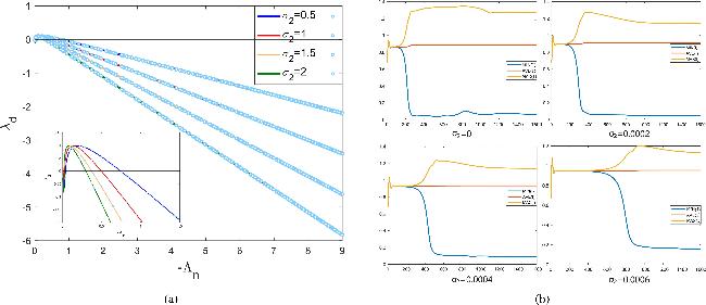
In figure 5, we explore the changes in λd and the evolution of infected density as the second-order coupling strength σ2 increases. In figure 5(a). As σ2 increases, the instability band (i.e. the range of Laplacian eigenvalues Λn with λd > 0) becomes narrower, indicating a reduction in the number of unstable modes. And the lower left corner shows a magnified image. In figure 5(b), we observe that as the coupling strength σ2 increases from 0 to 0.0006, the stabilization time of the pattern gradually lengthens.
Immediately thereafter, we will focus on the influence of key parameters in higher-order interactions on the formation of Turing patterns.
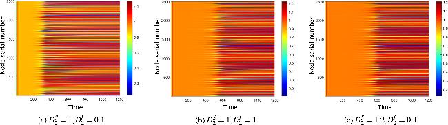
In figure 6, we examine the effect of the second-order diffusion coefficients ${D}_{2}^{S}$ and ${D}_{2}^{I}$ on the pattern evolution process. It can be observed that increasing either coefficient leads to a noticeable prolongation of the stabilization time of the spatial pattern. Combined with the results in figure 5(b), this indicates that the presence of higher-order diffusion tends to slow down the convergence to a steady state in the system dynamics.
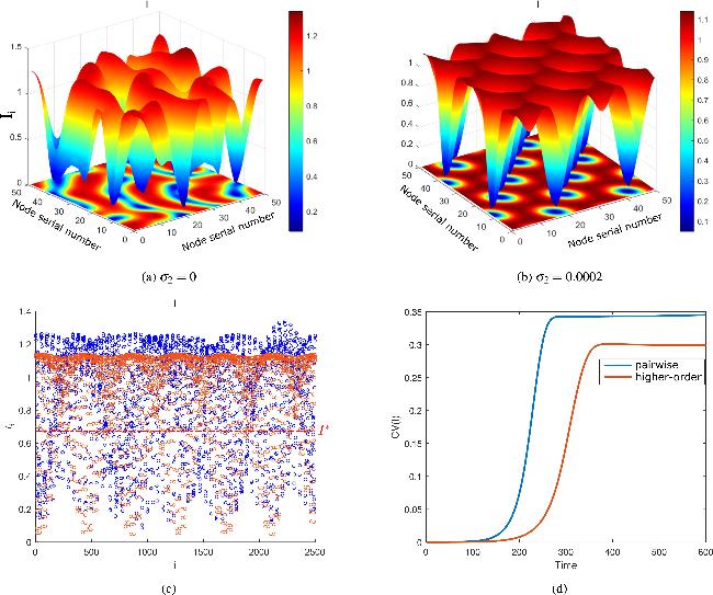
In figure 7, we define the discrete coefficient $\mathrm{CV}(x)=\sigma /\bar{x}$, where σ and $\bar{x}$ denote the standard deviation and mean, respectively. A small higher-order diffusion term (σ2: 0 → 0.0002) markedly alters the pattern. At t = 1000 (figures 7(a)–(b)), the barred low-density region transforms into a spiky structure with reduced peak height. Figure 7(c) shows infected densities at t = 1000: blue dots (pairwise only) and orange dots (with 3-body interactions) indicate that higher-order interactions lower infection density. Figure 7(d) plots the time evolution of CV(I) from t = 0 to 600, revealing that higher-order interactions reduce spatial heterogeneity and delay convergence, thus affecting both transient dynamics and steady states of infection spread.
4.2. Influence of advection
In the numerical simulations that follow, if not otherwise specified, the advective methods of susceptible individuals and infected individuals are figures 3(a) and (b) for one-way advection, figure 3(c) for isotropic advection, and figure 3(d) for reverse advection. Next we still use the parameters fixed in part A of this section and fix σ2 = 0.0004.
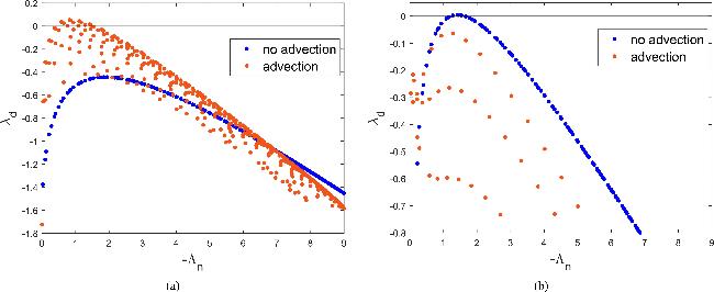
In figure 8, there is a fixed set of parameters. Specifically, A = 0.9, d = 0.24, μ = 0.02, γ = 0.54, α = 0.01, k2 = 0.9, ${D}_{1}^{S}={D}_{2}^{S}=5$, ${D}_{1}^{I}={D}_{I2}=0.1$, σ1 = 1 and σ2 = 0.1. Similar to figure 4, this side λd is defined as the largest real part of the eigenvalues in equations (14) and (19), i.e. ${\lambda }_{d}=\max \,\rm{Re}\,({\lambda }_{i})$ (where λi is a function of Λn and i = 2, 3). We still choose the eigenvalues of L1 as the horizontal coordinates, and since the value of λ3 in equation (19) is also affected by the advection matrix, the image of the dispersion relation of λ3 exhibits an obvious oscillatory pattern. Here, the blue points indicate diffusion relations without advection, while the orange points include advection. It is observed that advection has a dual effect on the formation of Turing patterns. In figure 8(a), we set k1 = 0.25, d1 = 8, d2 = 0. Observations show that the introduction of advection introduces Turing instability. In figure 8(b), we set k1 = 0.22, d1 = 0, d2 = 8 and observe that the introduction of advection suppresses the Turing instability.
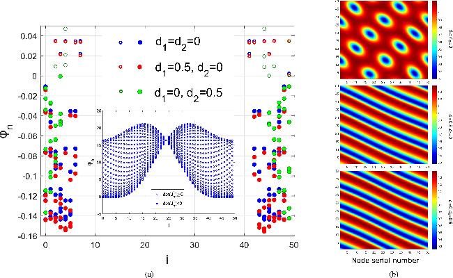
In figure 9, we examine how different advection configurations affect φn and infected density. From equation (21), advection-induced Turing instability requires φn < 0. The horizontal axis index i denotes spatial perturbation modes (i, j) from the eigenvalues Λi,j of the first-order Laplacian and advection matrices, with j fixed and i varying to represent spatial frequency in one direction. Multiple φn values for each i are shown vertically. In figure 9(a), point colors indicate advection type: blue (none), red (S-only), green (I-only). Solid symbols satisfy φn < 0; hollow do not. Advection on S lowers φn, increasing unstable modes, while advection on I raises φn, reducing instability. Figure 9(b) shows infected density for the same parameters: with sufficient advection, low-density zones shift from point-like to strip-like patterns, indicating that advection modulates both the extent and morphology of spatial heterogeneity.
Figure 9. Investigate the influence of advection methods on the Φn and patterns.
Next, two typical advective configurations are considered to explore their influence on Turing pattern formation.
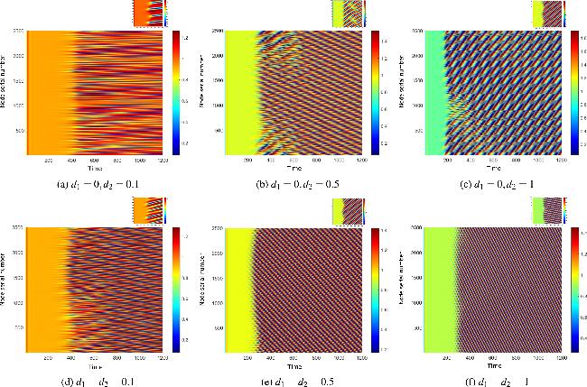
Figure 10 shows the infected density evolution over 1200 time units for all 2500 nodes, with a localized zoomed-in view in the upper right corner illustrating the first 100 nodes over 800 time units. Figures 10(a)–(c) apply one-way advection, while figures 10(d)–(f) implement reverse advection. In both cases, the stabilization time of node-level infected density is significantly shortened as the advection intensity increases. Localized observations further indicate that the upward inclination and density of the striped low-density regions tend to increase with stronger advection. These results suggest that increased advection intensity accelerates the transient dynamics and alters the spatial orientation of low-density regions in the infection field.
Figure 10. The evolution process of the infected density under two advection modes with different advection strength.
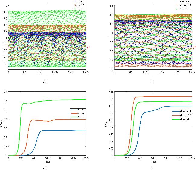
Figure 11 presents the scatter plots of infected density at time 1000 and the temporal evolution of CV(I) over 1200 time units. Figures 11(a), (b) correspond to one-way advection for susceptible individuals, and figures 11(c), (d) show reverse advection. In figure 11(a), increasing advection intensity leads to a broader distribution and an enhanced peak of infected density. A similar trend is observed in figure 11(b) under reverse advection. In figure 11(c), CV(I) increases monotonically with advection intensity, accompanied by a shortened stabilization time. Figure 12(d) exhibits a non-monotonic behavior of CV(I) (first increasing and then decreasing), with a similar shortening of the stabilization period.
Figure 12. Investigate the influence of advection methods on the Turing patterns at time 600.
These results demonstrate that advection intensity influences both the degree of spatial heterogeneity and the duration of epidemic system. Specifically, stronger advection can lead to more dispersed patterns and faster convergence to steady-state configurations.
Next, let us explore another scenario where we fix the following parameters A = 0.9, d = 0.24, μ = 0.02, γ = 0.54, α = 0.01, k1 = 0.07, k2 = 0.9, ${D}_{1}^{S}={D}_{2}^{S}=3$, ${D}_{1}^{I}={D}_{2}^{I}=0.1$ and σ1 = 1. It can be observed that the density of Infected under this set of parameters shows more low-density areas. We will explore the effects of advection mechanisms in this case.
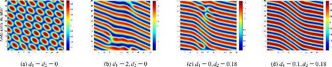
In figure 12, we analyze the effects of different advective configurations on the formation of the patterns. We observe that, for a certain convective intensity, the infected density pattern evolves from point-like high-density zones to bar-like high-density zones. This suggests that the introduction of advection can expand the spatial extent of high-density regions in the patterns.
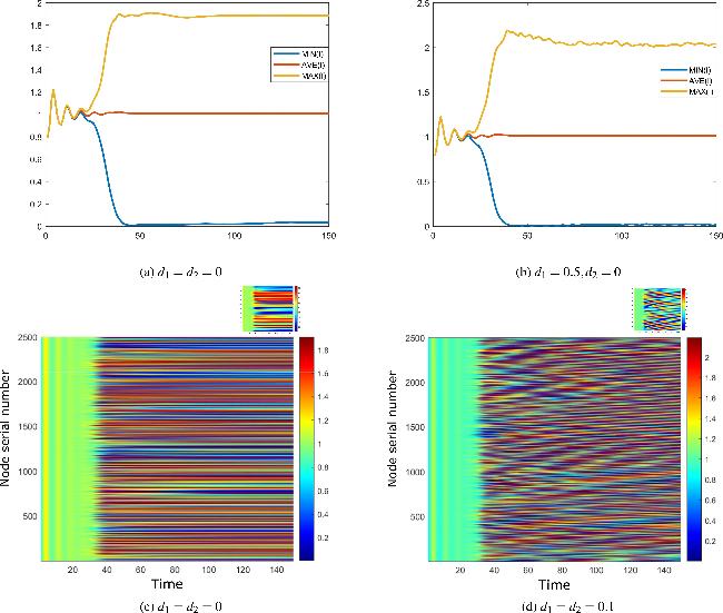
We now focus on the influence of advection on the temporal and spatial dynamics of Turing patterns. Figure 13 compares the infected density evolution in systems with and without advection. Figures 13(a), (c) correspond to simulations without advection, while figures 13(b), (d) include reverse advection. Notably, when advection is introduced [figure 13(b)], the peak infected density increases significantly, and the system exhibits mild oscillations even after reaching a quasi-steady state. In contrast to the horizontally ordered distribution in figures 13(c), (d) displays a more irregular structure, where the low-density strips of infected individuals appear tilted to the upper right, forming an asymmetric and spatially complex pattern. This observation suggests that advection may contribute to the emergence of disordered or chaotic structures in the spatial distribution of infected density.
Figure 13. The influence of d2 = 2 on the evolution process of the density for infected individuals.
4.3. Real data simulation
To verify the validity of the epidemic model developed above, we carry out numerical simulations using weekly influenza A case data collected from medical institutions across Japan's 47 prefectures, spanning from January 1, 2024 to January 16, 2025.
To incorporate regional heterogeneity in transmission dynamics, we consider a heterogeneous PDE system defined on the empirical inter-prefectural commuting network. The higher-order structure of the empirical network is constructed consistently with the generalized definitions introduced in the theoretical framework. In particular, the second-order adjacency tensor A2 is defined by ${A}_{ijk}^{2}=1$, whenever nodes (i, j, k) form a 2-simplex, and ${A}_{ijk}^{2}=0$ otherwise. Based on A2, the generalized second-order Laplacian matrix ${\widetilde{L}}^{2}$ is given by
which represent local demographic and transmission characteristics.
All parameters are treated as node-dependent constants and are jointly inferred together with the neural network representation of the solution fields.
For clarity, the heterogeneous system can also be written explicitly for each prefecture i as
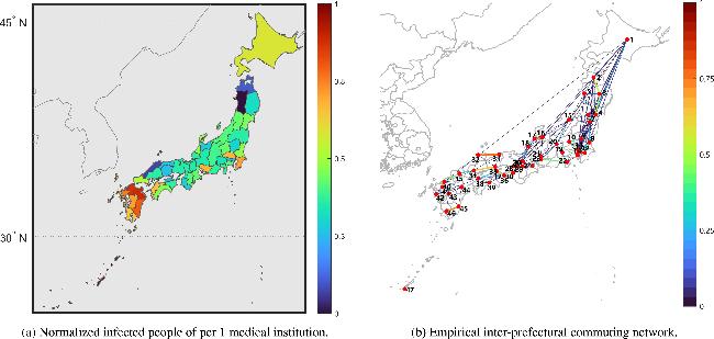
Figure 14(a) shows a heat distribution based on the normalized number of infected people per medical institution, with the color scale indicating the normalized values. (Data from https://www.naturalearthdata.com/downloads/10m-cultural-vectors/) figure 14(b) depicts the empirical inter-prefectural commuting network, where nodes represent prefectures and directed edges indicate normalized human mobility flows, with the color scale representing connection strength. (Data from https://www.e-stat.go.jp/dbview?sid=0004019526)
Figure 14. Heat map and commuting network for Japan's 47 prefectures.
While the triangular lattice adopted in the theoretical analysis provides a mathematically elegant and analytically tractable setting, it cannot fully capture the geographical complexity and social heterogeneity of real-world human interactions. Its primary role in our framework is to isolate and visualize the influence of higher-order spatial interactions—particularly directional advection—in a controlled environment, thereby enabling clearer identification of pattern-forming instabilities and spatial modes. To move beyond the limitations of such idealized settings, we extend our model to a more realistic spatial configuration by incorporating empirical inter-prefectural commuting data for Japan's 47 prefectures. In epidemiological modeling, commuting networks are widely recognized as a natural proxy for the pathways along which infectious diseases spread, since regular population flows between regions directly facilitate pathogen transmission. Figure 14(b) visualizes this empirical commuting network, where nodes correspond to prefectures and directed edges represent population flows. Using official statistics, we construct a directed and weighted mobility network in which edge directionality represents net human flows and raw mobility counts are converted to normalized weights via a proportional scaling method [42]:
where Mij denotes the observed commuting volume from prefecture i to j. This normalization ensures that edge weights reflect the proportion of outbound commuters from each prefecture, thereby preserving relative movement intensities. The resulting weighted migration matrix generalizes the unweighted advection matrix used in the theoretical model, embedding it in a geographically grounded and empirically informed structure. This modification enables the model to account for spatial asymmetry, directional spread, and heterogeneous connectivity, thereby bridging the gap between abstract theory and real-world epidemic dynamics.
In scientific research and engineering practice, neural networks have been extensively applied to data fitting and the prediction of complex systems [39, 40, 43–47]. We then employ PINNs [39, 40] to fit the full heterogeneous-parameter PDE system to the data from all 47 prefectures simultaneously. This method integrates the observed epidemiological data with the governing partial differential equations, ensuring consistency with both empirical patterns and theoretical dynamics. Unlike traditional curve-fitting methods or purely data-driven neural networks, PINNs impose physical constraints that help avoid overfitting and improve generalizability, especially in sparse or noisy regions of the dataset. We note that, similar to many gradient-based optimisation methods, the training process of PINNs may exhibit sensitivity to initial parameter values. However, the primary purpose of employing PINNs here is not to locate a globally optimal parameter set, but rather to fit our proposed higher-order network epidemic model by using commuting networks and real-world epidemic data. Crucially, systems incorporating higher-order interactions demonstrate superior fitting accuracy compared to their pairwise interaction counterparts.
Specifically, the PINN takes as input the concatenation of the node identity vector ${e}_{i}\in {{\mathbb{R}}}^{47}$ (the i-th standard basis vector) and time tn, and outputs the state variables (Si(tn), Ii(tn)) for all prefectures. The first-order diffusion is governed by L1, while the higher-order diffusion is governed by ${\widetilde{L}}^{2}$ constructed from the adjacency tensor A2. For each node i, the diffusion items are defined component-wise as
where σ(1,i) and σ(2,i) denote the node-dependent first- and second-order coupling strengths, respectively. The reaction items follow the model equations defined in model (1), which are given explicitly by
$\begin{eqnarray*}\begin{array}{r}\begin{array}{rcl}{ \mathcal F }({S}_{i},{I}_{i}) & = & {A}_{i}-{d}_{i}{S}_{i}-\frac{({k}_{1,i}{I}_{i}+{k}_{2,i}{I}_{i}^{2}){S}_{i}}{1+{\alpha }_{i}{I}_{i}^{2}},\\ { \mathcal G }({S}_{i},{I}_{i}) & = & \frac{({k}_{1,i}{I}_{i}+{k}_{2,i}{I}_{i}^{2}){S}_{i}}{1+{\alpha }_{i}{I}_{i}^{2}}-({d}_{i}+{\mu }_{i}+{\gamma }_{i}){I}_{i}.\end{array}\end{array}\end{eqnarray*}$
Using automatic differentiation to compute temporal derivatives, the physics residuals at time sample tn are
$\begin{eqnarray*}\begin{array}{r}\begin{array}{rcl}{R}_{1,i}({t}_{n}) & = & {\partial }_{t}{S}_{i}({t}_{n})-({{ \mathcal D }}_{S,i}({t}_{n})+{ \mathcal F }({S}_{i}({t}_{n}),{I}_{i}({t}_{n})),\\ {R}_{2,i}({t}_{n}) & = & {\partial }_{t}{I}_{i}({t}_{n})-({{ \mathcal D }}_{I,i}({t}_{n})+{ \mathcal G }({S}_{i}({t}_{n}),{I}_{i}({t}_{n})).\end{array}\end{array}\end{eqnarray*}$
The physics-informed loss is defined as the mean squared residual over all nodes and time samples:
where ϵ = 10−3 prevents the unobserved variable from drifting and ${I}_{i}^{{\rm{o}}{\rm{b}}{\rm{s}}}({t}_{n})$ denotes the observed value of Ii(tn) at time tn.
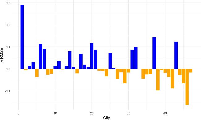
To assess the contribution of higher-order spatial operators to model performance, we compare fits with and without the inclusion of these terms figure 15 illustrates the change in root mean square error (RMSE) across all prefectures; orange bars indicate a reduction in RMSE when higher-order terms are included. Notably, 57.45% of the prefectures experience improved fit accuracy with the inclusion of higher-order interactions, validating their relevance in real-world modeling.
Figure 15. The change in RMSE across all prefectures.
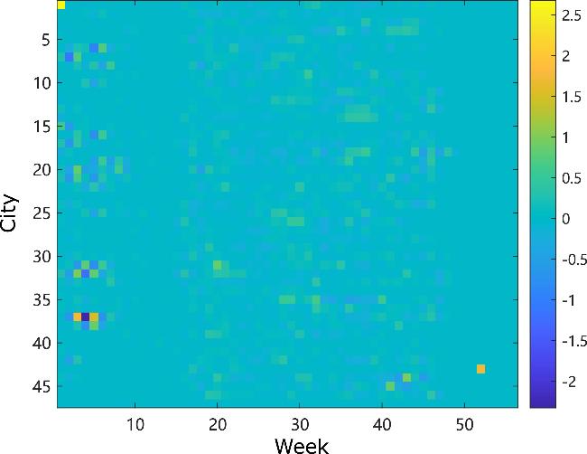
Figure 16 further presents the weekly distribution of fitting errors across prefectures over 56 weeks in a heatmap format, where darker colours denote lower errors and higher fitting quality. This visualisation clearly demonstrates the significant role of higher-order spatial operators in enhancing spatio-temporal modelling precision.
Figure 16. Heatmap of weekly fit errors across 56 weeks for all 47 prefectures.
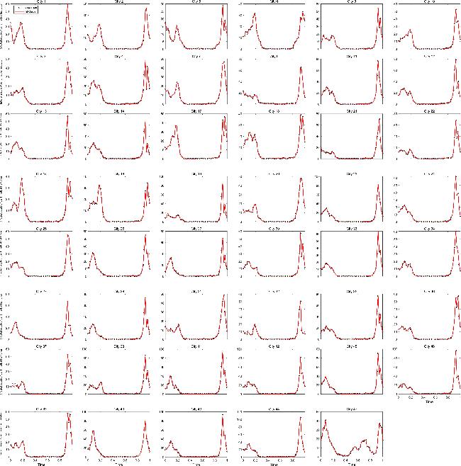
Figure 17 presents a comparison of the fitted curves with actual observed values across all 47 prefectures, with results for typical groups also displayed separately. The high degree of agreement between the curves indicates that the model demonstrates good overall fitting performance.
Figure 17. Fitted curves versus real data for all 47 prefectures.
In summary, the introduction of higher-order interactions enhances the model's fitting accuracy and consistency across diverse regions.
5. Conclusion
In this paper, we develop a networked reaction–diffusion infectious disease propagation model on a discrete network space, incorporating higher-order interactions and advection mechanisms. The triangular lattice topology used in the theoretical analysis is chosen solely for its analytical tractability and visual clarity, enabling controlled exploration of the interplay between these mechanisms, rather than as a direct representation of real-world contact structures. By analyzing the necessary conditions for Turing instability under three mechanisms, we identify multiple regulatory pathways for transmission dynamics.
On the one hand, three-body interactions significantly prolong the stabilization period of infectious diseases and inhibit the transition of low-density infected zones from punctate to stripe patterns. On the other hand, the advection mechanism exhibits a spatially selective double-edged effect—when high-density infected areas dominate, advection promotes stripe merging to accelerate spread, whereas when low-density areas dominate, it suppresses spread. The synergy of these mechanisms overcomes the limitations of traditional localized models.
Finally, application to a real-world commuting network demonstrates that incorporating higher-order spatial interactions significantly improves the fitting accuracy of the proposed PINN-based model.
The above work deepens our understanding of the mechanisms underlying Turing pattern formation, providing valuable insights for the study of reaction–diffusion systems. Future research will investigate how higher-order network structures influence dynamical processes and renormalization [48, 49], thereby advancing infectious disease prediction models toward high-dimensional spatiotemporal evolution.
Appendix Prooerties of the triangular lattice torus network
Mathematically, Zhu [30] has obtained the eigenvalues of the composite torus network, which we generalize to the triangular lattice torus network and give the eigenvalues of the first-order Laplace matrix. We define a permutation matrix ${{\rm{\Gamma }}}_{{N}_{0}}$ (${{\rm{\Gamma }}}_{{N}_{0}}^{{\bf{T}}}={{\rm{\Gamma }}}_{{N}_{0}}^{-1}$ and ${N}_{0}=\sqrt{N}$),
The eigenvalues of this matrix are ${\zeta }_{1}^{{\rm{\Gamma }}},\cdots \,,{\zeta }_{{N}_{0}}^{{\rm{\Gamma }}}$ and its corresponding right eigenvectors are ${\beta }_{1},\cdots \,,{\beta }_{{N}_{0}}$ respectively, i.e. ${\rm{\Gamma }}{\beta }_{n}={\zeta }_{n}^{{\rm{\Gamma }}}{\beta }_{n}$$\left(n=1,\cdots \,,{N}_{0}\right)$. By transposing the matrix, left-multiplying the inverse matrix, etc, we can obtain
where ∘ denotes the linear transformation L1 to acting on the vector α. Let us take ${{\rm{\Psi }}}_{i,j}\triangleq {\beta }_{i}\otimes {\beta }_{j}^{{\bf{T}}}$, α = $\Psi$i,j(i, j = 1, 2, ⋯ , N) and bring them into equation (A3).
Next, we construct the advection matrix and its eigenvalues are derived as an example for a 4 × 4 network. Then the results will be generalized to general N0 × N0 networks.
According to permutation matrix Γ, we can derive the advection matrix in figure 18 as follow
Declaration of competing interest The authors declare that they have no known competing financial interests or personal relationships that could have appeared to influence the work reported in this paper. Wenlong Zhang: Writing—original draft, Formal analysis, Data curation. Xuerui Zhu: Conceptualization. Linhe Zhu: Writing—original draft, Methodology, Conceptualization, Formal analysis.
This research is supported by National Natural Science Foundation of China (Grant No. 12002135), China Postdoctoral Science Foundation (Grant No. 2023M731382), Higher Education Teaching Reform of Jiangsu University (Grant No. 2025JGYB018), and Jiangsu University 2025 College Students Innovative Training Program Project (Grant No. X2025102990815).
LiB X, ZhuL H>2024 Turing instability analysis and parameter identification based on optimal control and statistics method for a rumor propagation system Chaos34 053143
KristinaM, MartinW, TimC>2024 Hybrid PDE–ODE models for efficient simulation of infection spread in epidemiology Proc. R. Soc. A481 20240421
3
GlimmT, KaźmierczakB, NewmanS A, BhatR>2023 A two-galectin network establishes mesenchymal condensation phenotype in limb development Math. Biosci.365 109054
KermackW O, McKendrickA G>1927 A contribution to the mathematical theory of epidemics Proc. R. Soc. A115 700 721
5
HuJ L, ZhuL H>2022 Analysis of Turing patterns and amplitude equations in general forms under a reaction–diffusion rumor propagation system with Allee effect and time delay Inf. Sci.596 501 519
SalmanS M, HanR J>2024 Spatiotemporal patterns in a space–time discrete SIRS epidemic model with self- and cross-diffusion Int. J. Bifurcation Chaos34 2450098
ZhaiS D, LuoG Q, HuangT, WangX, TaoJ L, ZhouP>2021 Vaccination control of an epidemic model with time delay and its application to COVID-19 Nonlinear Dyn.106 1279 1292
DongS, XuL L, AY, LanZ Z, XiaoD, GaoB>2023 Application of a time-delay SIR model with vaccination in COVID-19 prediction and its optimal control strategy Nonlinear Dyn.111 10677 10792
SimmonsE S G, CooleyA M, PuzeyJ R, SmithG D C>2023 A multigenerational turing model reproduces transgressive petal spot phenotypes in hybrid mimulus Bull. Math. Biol.85 120
DaiS Y, ZhuL H, HeL, DongY J>2026 Dynamics and control of infectious diseases on complex networks: a theoretical and empirical study J. Math. Anal. Appl.557 130334
LiB X, ZhuL H>2024 Turing instability analysis of a reaction–diffusion system for rumor propagation in continuous space and complex networks Inf. Process. Manage.61 103621
ShaH Y, ZhuL H>2025 Dynamic analysis of pattern and optimal control research of rumor propagation model on different networks Inf. Process. Manage.62 104016
ZhuL H, DingY, ShenS L>2025 Green behavior propagation analysis based on statistical theory and intelligent algorithm in data-driven environment Math. Biosci.379 109340
ZhuL H, ZhengT T>2025 Pattern dynamics analysis and application of West Nile virus spatiotemporal models based on higher-order network topology Bull. Math. Biol.87 121
WuP, SalmaniwY, WangX N>2024 Threshold dynamics of a reaction–advection–diffusion schistosomiasis epidemic model with seasonality and spatial heterogeneity J. Math. Biol.88 76
MuoloR, GiambagliL, NakaoH, FanelliD, CarlettiT>2024 Turing patterns on discrete topologies: from networks to higher-order structures Proc. R. Soc. A480 20240235
35
LiX, HeR, XiY X, XueY K, WangY F, LuoX F>2024 The increasing strength of higher-order interactions may homogenize the distribution of infections in Turing patterns Chaos Solitons Fractals178 114369
BalcanD, ColizzaV, GoncalvesB, HuH, RamascoJ J, VespignaniA>2009 Multiscale mobility networks and the large scale spreading of infectious diseases Proc. Natl Acad. Sci. USA106 21484 21489
GuoZ M, ZouY, SunC J, JayanH, JiangS Q, El-SeediH R, ZouX B>2024 Nondestructive determination of edible quality and watercore degree of apples by portable Vis/NIR transmittance system combined with CARS-CNN J. Food Meas. Charact.18 4058 4073
NunekpekuX, ZhangW, GaoJ Y, AdadeS Y S, ChenQ S>2025 Gel strength prediction in ultrasonicated chicken mince: fusing near-infrared and Raman spectroscopy coupled with deep learning LSTM algorithm Food Control168 110916