


1. Introduction
To implement the precise measurement using quantum interferometry, the long coherent time of a quantum sensor is typically required [1–3]. Electronic spins can be implemented as quantum sensors [4] due to weak magnetic coupling with electromagnetic noise. Compared to traditional solid-state spins [4], here the considered spin of electron floating on liquid helium [5–8] may exhibit relatively long coherent times, because the inert liquid 4He serves as an ideal substrate without a thermal spin-bath. Note that, the electron floating on the liquid helium is due to the Pauli exclusion principle which results in a barrier at the helium liquid surface [9]. At the same time, there is a long-range attractive force due to electronic image charge inside the liquid helium, and therefore the electron floats on liquid helium surface [10–13]. For lateral motion, the test electron can be trapped by using the electrostatic field generated by the artificial micro-electrodes beneath the liquid helium surface [14–17].
As mentioned above, electronic spin is a magnetic moment and thus also exhibits the weak coupling to the signal electromagnetic field. This results in the difficulty of single spin qubit detection. In 2010, Schuster et al proposed a theoretical approach to detect a single spin by using the spin–orbit coupling and the electric dipole interaction between the orbital state of trapped electron and a superconducting resonator [14]. In recent years, they have experimentally detected the charge degree of freedom of single trapped electron on liquid helium by using the superconducting resonator [15–18].
Here, we show an ac Stark effect [19] of the electronic spin trapped on liquid helium, which is induced by the electric field of gigahertz (GHz) microwave rather than its weak magnetic field. Similar to the proposal [14], a dc current on the micro-electrode (also used for trapping the electron) is arranged to generate the strong coupling between the electronic spin and the lateral orbital state. With the help of this spin–orbit coupling, we show that the inputting microwave can generate an effective Stark effect of the spin due to the strong electric dipole interaction referring to the charge degree of freedom of this system. During this process, the inputting microwave neither excites the cavity field nor the orbital states of the trapped electron. Therefore, the decay in the present cavity-QED system is greatly suppressed, and then the famous Ramsey interferometry can be suitable for implementing the precise measurements for the inputting microwave. As the superconducting resonators work within the GHz regime, the present study shows a new way for implementing the single photon detection of GHz microwaves.
2. Trapped electron in a superconducting resonator
The micro-electrodes structure shown by figure 1 enables to trap the surface-binding electron inside a superconducting resonator. Within the Cartesian coordinate system showed by figure 1(a), the electrostatic potential generated by the designed electrodes structure can be expanded as a Taylor series: ${\phi }_{0}(z,x,y)\approx y{E}_{y}+{z}^{2}{E}_{z}^{{\prime} }+{x}^{2}{E}_{x}^{{\prime} }+{y}^{2}{E}_{y}^{{\prime} }$ in the small regime of (z, x, y) → (0, 0, 0) [20]. Here, we have used the geometric symmetry of the present line-electrodes structure, i.e., φ0(z, x, y) = φ0(z, − x, y) and φ0(z, x, y) = φ0(z, x, − y). The constant coefficients Ey, ${E}_{z}^{{\prime} }$, ${E}_{x}^{{\prime} }$, and ${E}_{y}^{{\prime} }$ can be numerically solved by the so-called Moment Method in Computational Electromagnetics [21]. For example, ${E}_{z}^{{\prime} }\approx 4.49\times 1{0}^{-3}V/{(\,\rm{\unicode{x000B5}m}\,)}^{2}$, ${E}_{x}^{{\prime} }\approx 4.54\times 1{0}^{-3}V/{(\,\rm{\unicode{x000B5}m}\,)}^{2}$, ${E}_{y}^{{\prime} }\approx -9.08\times 1{0}^{-3}V/{(\,\rm{\unicode{x000B5}m}\,)}^{2}$, within the structure showed by figure 1(a), and where V is an arbitrary voltage. Beyond the harmonic oscillator potential limited within the small regime around (0, 0, 0), figure 1(b) shows a complete 2D potential well for laterally trapping the electron on liquid helium.
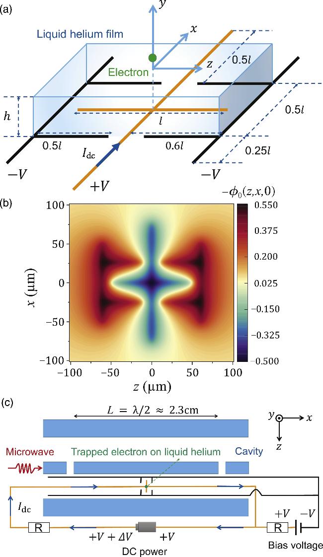
Figure 1. (a) Electrode-structure at plane y = − h for trapping the electron on the surface of liquid helium, with ±V being the bias voltages. Where l = 100 µm is the length of the positive electrode in the z direction, and h = 4.8 µm is the height of the liquid helium. Additionally, the magnetic field B generated by the dc current Idc is applied to generate the spin qubit and also the spin–orbit coupling. (b) The numerical solution of electrostatic potential φ0(z, x, 0) generated by the present electrode-structure. (c) The electron trap is placed into a superconducting resonator for manipulating and detecting the spin qubit based on the cavity-QED described by the text. |
Note that, (i) with the controllable bias-voltage V, the captured electron by the above potential well shall decay into the vibrational ground state, which corresponds to the lowest energy state of the electron's motion, modeled as a harmonic oscillator in the 10 mK environment [15–17]. Thus, we treat the trapped electron as a harmonic oscillator with the frequency ${\omega }_{b}=\sqrt{2e{E}_{z}^{{\prime} }/{m}_{e}}\approx 2\pi \times 6.45\,{\rm{GHz}}$, by setting the bias-voltage V ≈ 1.04 Volt. Where me ≈ 9.1 × 10⁻³¹ kg and e ≈ 1.6 × 10⁻¹⁹ C are the mass and charge of an electron, respectively. (ii) The vertical orbital motions of the surface-binding electron work within the millimeter wave range, and thus are negligible in the present GHz cavity-QED system.
To realize the coupling between the spin and horizontal vibration of trapped electron, we apply a x-directional dc current Idc in one of the micro-electrodes, as shown in figure 1(a). The generated local magnetic field for the trapped electron (of y ≪ z ≪ h) can be approximately written as B ≈ B0[ez − (z/h)ey], with B0 = μ0Idc/(2πh), and where μ0 = 4π × 10−7 T · m/A is the vacuum permeability. ez and ey are unit vectors in the z and y directions respectively.
The spin-Zeeman splitting due to the above static magnetic field is given by 1 ) defines a spin qubit with the transition frequency ωs = 2μBB0/ℏ, and where μB ≈ 9.3 × 10⁻²⁴ Am2 stands for the Bohr magneton. Considering Idc = 5.47 A, we have ωs ≈ 2π × 6.395 GHz, and consequently, the spin–orbit coupling term zσy can be accessible for the GHz superconducting resonator [15–17].
$\begin{eqnarray}\begin{array}{r}{\mu }_{{\rm{B}}}\sigma \cdot {\boldsymbol{B}}\approx \frac{\hslash {\omega }_{s}}{2}{\sigma }_{z}-\frac{\hslash {\omega }_{s}}{2}\frac{z{\sigma }_{y}}{h},\end{array}\end{eqnarray}$
with σz = ∣ ↑ ⟩⟨ ↑ ∣ − ∣ ↓ ⟩⟨ ↓ ∣ and σy = ∣ ↑ ⟩⟨ ↓ ∣ + ∣ ↓ ⟩⟨ ↑ ∣ being the well-known Pauli operators. As is well-known, ∣ ↑ ⟩ and ∣ ↓ ⟩ express the two eigenstates of the spin-1/2 particle. Obviously, the first term ℏωsσz in equation (3. Unitary transformation approach for deriving Spin ac Stark effect
According to the lateral harmonic oscillator potential and the spin–orbit coupling, the Hamiltonian of the spin-cavity system can be written as 2 ) describes the effective spin–orbit coupling, with σ+ = ∣ ↑ ⟩⟨ ↓ ∣ and σ− = ∣ ↓ ⟩⟨ ↑ ∣ being the spin raising operator and lowering operator, respectively. Numerically, gbs = ωsz0/(2h) ≈ 2π × 6.25 MHz, with ${z}_{0}=\sqrt{\hslash /(2{m}_{e}{\omega }_{b})}$ being the positional zero-point fluctuation of electronic orbital motion.
$\begin{eqnarray}\begin{array}{rcl}{H}_{0} & = & \hslash {\omega }_{a}{a}^{\dagger }a+\hslash {\omega }_{b}{b}^{\dagger }b+\frac{1}{2}\hslash {\omega }_{s}{\sigma }_{z}\\ & & +\hslash {g}_{ba}({a}^{\dagger }b+a{b}^{\dagger })+\hslash {g}_{bs}(b{\sigma }_{+}+{b}^{\dagger }{\sigma }_{-}).\end{array}\end{eqnarray}$
The first term ℏωaa†a describes the energy of a bare cavity-mode of frequency ωa = 2π × 6.4 GHz [15], with creation and annihilation operators a† and a, respectively. Similarly, the second term ℏωbb†b describes the lateral harmonic oscillator of the trapped electron on liquid helium, with aforementioned frequency ωb ≈ 2π × 6.45GHz. The third term defines a spin qubit. Under the well-known rotating wave approximation (RWA), the fourth term describes the standard electric dipole interaction between the harmonic oscillator and the cavity mode, with gba = 2π × 5 MHz being the coupling strength, which has been experimentally observed in the study of reference [15]. Again applying the RWA, the last term in equation (Now, we consider the resonator being driven by a microwave (a signal to be detected). Thus, the total Hamiltonian becomes 3 ) describes the coupling between the microwave field and the cavity [22], with gac representing the coupling strength between them, which also has been observed in the reference [15]. Based on the present equation (3 ), a spin Stark effect induced by the incoming signal wave can be derived by using the following three unitary transformations.
$\begin{eqnarray}\begin{array}{r}H={H}_{0}+\hslash {\omega }_{c}{c}^{\dagger }c+{\rm{i}}\hslash {g}_{ac}(a{c}^{\dagger }-c{a}^{\dagger }),\end{array}\end{eqnarray}$
where c† and c are the bosonic creation and annihilation operators of the inputting microwave (to be detected). The third term in the above equation (First, we apply the unitary transformation [23]:
$\begin{eqnarray}\begin{array}{r}{U}_{1}=\exp \left[\frac{{g}_{ba}}{{{\rm{\Delta }}}_{ba}}(a{b}^{\dagger }-{a}^{\dagger }b)+\frac{{g}_{bs}}{{{\rm{\Delta }}}_{bs}}({b}^{\dagger }{\sigma }_{-}-b{\sigma }_{+})\right],\end{array}\end{eqnarray}$
to solve the Schrödinger equation. Here, Δba = ωb − ωa is the detuning between the resonator and the harmonic oscillator of trapped electron, while Δbs = ωb − ωs represents the detuning between the spin and the harmonic oscillator. Considering the large detuning gba ≪ Δba and gbs ≪ Δbs, we have the first effective Hamiltonian $\begin{eqnarray}\begin{array}{rcl}{H}_{1}/\hslash & = & {U}_{1}(H/\hslash ){U}_{1}^{\dagger }\\ & \approx & {\omega }_{a1}{a}^{\dagger }a+{\omega }_{b1}{b}^{\dagger }b+\frac{1}{2}{\omega }_{s1}{\sigma }_{z}+{\omega }_{c}{c}^{\dagger }c\\ & & -{g}_{as}({a}^{\dagger }{\sigma }_{-}+a{\sigma }_{+})\\ & & +{\rm{i}}{g}_{ac}(a{c}^{\dagger }-{a}^{\dagger }c)+{\rm{i}}{g}_{bc}(b{c}^{\dagger }-{b}^{\dagger }c)-{\omega }_{bs}{\sigma }_{z}{b}^{\dagger }b,\end{array}\end{eqnarray}$
by neglecting the terms involving small values ${({g}_{ba}/{{\rm{\Delta }}}_{ba})}^{2}$ and ${({g}_{bs}/{{\rm{\Delta }}}_{bs})}^{2}$. As mentioned above, ${\omega }_{a1}={\omega }_{a}-({g}_{ba}^{2}$/Δba), ${\omega }_{b1}={\omega }_{b}+({g}_{ba}^{2}$/Δba), ${\omega }_{s1}={\omega }_{s}-({g}_{bs}^{2}$/Δbs), are the re-normalized eigenfrequencies of cavity, harmonic oscillator, and spin, respectively. Moreover, gas = gbagbs(Δba + Δbs)/2ΔbaΔbs represents the spin-cavity coupling strength, gbc = gbsgac/Δbs describes the coupling between the inputting external field and the harmonic oscillator. Finally, ${\omega }_{bs}={g}_{bs}^{2}/{{\rm{\Delta }}}_{bs}$ describes the energy-level splitting of spin qubit, which depends on the state of harmonic oscillator.Following the above Hamiltonian of equation (5 ), we define a new detuning Δas = ωa1 − ωs1, and proceed on the large-detuning, i.e., gas ≪ Δas. Applying the second unitary transformation
$\begin{eqnarray}\begin{array}{r}{U}_{2}=\exp \left[\frac{{g}_{as}}{{{\rm{\Delta }}}_{as}}({a}^{\dagger }{\sigma }_{-}-a{\sigma }_{+})\right],\end{array}\end{eqnarray}$
results in the new effective Hamiltonian $\begin{eqnarray}\begin{array}{rcl}{H}_{2}/\hslash & = & {U}_{2}({H}_{1}/\hslash ){U}_{2}^{\dagger }\\ & \approx & {\omega }_{a1}{a}^{\dagger }a+{\omega }_{b1}{b}^{\dagger }b+\frac{1}{2}{\omega }_{s2}{\sigma }_{z}+{\omega }_{c}{c}^{\dagger }c\\ & & +{\rm{i}}{g}_{ac}(a{c}^{\dagger }-{a}^{\dagger }c)\\ & & +{\rm{i}}{g}_{bc}(b{c}^{\dagger }-{b}^{\dagger }c)+{\rm{i}}{g}_{sc}({c}^{\dagger }{\sigma }_{-}-c{\sigma }_{+})\\ & & -{\omega }_{as}{\sigma }_{z}{a}^{\dagger }a-{\omega }_{bs}{\sigma }_{z}{b}^{\dagger }b,\end{array}\end{eqnarray}$
by neglecting the terms relating to small values ${({g}_{as}/{{\rm{\Delta }}}_{as})}^{2}$. Above, ${\omega }_{s2}={\omega }_{s1}-({g}_{as}^{2}/{{\rm{\Delta }}}_{as})$ is the new eigenfrequency of spin, and gsc = gasgac/Δas being the desired coupling between the inputting external field and spin. Additionally, ${\omega }_{as}={g}_{as}^{2}/{{\rm{\Delta }}}_{as}$ describes the energy-level splitting of spin qubit, which depends on the state of the cavity.Based on the Hamiltonian of equation (7 ), considering external field is large detuning not only with the cavity field but also with the electronic oscillator, i.e., gac ≪ (ωa1 − ωc) and gbc ≪ (ωb1 − ωc), the second line in equation (7 ) is still eliminable [24], and therefore 10 ), the terms relating to ${({g}_{sc}/{{\rm{\Delta }}}_{sc})}^{2}$ are neglected, as well as that made for Hamiltonian H1 and H2. It can be inferred that the incoming microwave does not excite the cavity modes or the electronic oscillator states, since the microwave field is decoupled from both under the multiple large detuning conditions mentioned above.
$\begin{eqnarray}\begin{array}{rcl}{H}_{2}/\hslash & \approx & {\omega }_{a1}{a}^{\dagger }a+{\omega }_{b1}{b}^{\dagger }b+\frac{1}{2}{\omega }_{s2}{\sigma }_{z}+{\omega }_{c}{c}^{\dagger }c\\ & & +{\rm{i}}{g}_{sc}({c}^{\dagger }{\sigma }_{-}-c{\sigma }_{+})-{\omega }_{bs}{\sigma }_{z}{b}^{\dagger }b-{\omega }_{as}{\sigma }_{z}{a}^{\dagger }a.\end{array}\end{eqnarray}$
Finally, taking the third unitary transformation $\begin{eqnarray}\begin{array}{r}{U}_{3}=\exp \left[{\rm{i}}\frac{{g}_{sc}}{{{\rm{\Delta }}}_{sc}}({c}^{\dagger }{\sigma }_{-}+c{\sigma }_{+})\right],\end{array}\end{eqnarray}$
we have $\begin{eqnarray}\begin{array}{rcl}{H}_{3}/\hslash & = & {U}_{3}({H}_{2}/\hslash ){U}_{3}^{\dagger }\\ & \approx & {\omega }_{a1}{a}^{\dagger }a+{\omega }_{b1}{b}^{\dagger }b+\frac{1}{2}{\omega }_{s3}{\sigma }_{z}+{\omega }_{c}{c}^{\dagger }c\\ & & -{\omega }_{sc}{\sigma }_{z}{c}^{\dagger }c-{\omega }_{as}{\sigma }_{z}{a}^{\dagger }a+{\omega }_{bs}{b}^{\dagger }b\\ & & -2{\rm{i}}({c}^{\dagger }{\sigma }_{-}-c{\sigma }_{+})({\omega }_{as}{a}^{\dagger }a-{\omega }_{bs}{\sigma }_{z}{b}^{\dagger }b)\\ & & -4({\sigma }_{+}{\sigma }_{-}+{\sigma }_{z}{c}^{\dagger }c)({\omega }_{as}{a}^{\dagger }a+{\omega }_{bs}{b}^{\dagger }b).\end{array}\end{eqnarray}$
with Δsc = ωs2 − ωc, gsc ≪ Δsc, ${\omega }_{s3}={\omega }_{s2}-({g}_{sc}^{2}/{{\rm{\Delta }}}_{sc})$ and ${\omega }_{sc}={g}_{sc}^{2}/{{\rm{\Delta }}}_{sc}$. In the present Hamiltonian of equation (Now, we consider a 10 mK dilution refrigerator, where both the cavity and the electron's orbital motions are cooled to their ground states, i.e.,⟨a†a⟩ = 0 and ⟨b†b⟩ = 0. Therefore, equation (10 ) reduces to 11 ) is valid within the regime where all degrees of freedom in the quantum system are in the large-detuning limit.
$\begin{eqnarray}\begin{array}{r}{H}_{{\rm{eff}}}/\hslash =\frac{1}{2}{\omega }_{s3}{\sigma }_{z}+{\omega }_{c}{c}^{\dagger }c-{\omega }_{sc}{\sigma }_{z}{c}^{\dagger }c,\end{array}\end{eqnarray}$
and where the last term describes the desired spin-Stark effect that is induced by the inputting microwave, which neither excite cavity nor the electronic oscillator. The effective Hamiltonian in equation (The proposed device, shown in figure 1, can easily achieve these conditions, due to the controllable bias-voltage and current. Table 1 lists some possible values that satisfy the above large detuning conditions in the derivation from equations (4 ) to (11 ). These values are close to the experimental parameters used in [15].
Table 1. Parameters satisfying the large detuning conditions used to derive the Hamiltonian of equation ( |
| ωa/2π | ωb/2π | ωs/2π | gba/2π | gbs/2π | gac/2π |
| 6.4 GHz | 6.45 GHz | 6.395 GHz | 5 MHz | 6.25 MHz | 16 MHz |
| Δba/2π | Δbs/2π | gas/2π | gbc/2π | ωbs/2π | Δas/2π |
| 50 MHz | 55 MHz | 0.6 MHz | 1.82 MHz | 0.7 MHz | 5.2 MHz |
| gsc/2π | ωas/2π | ωc/2π | Δsc/2π | ωsc/2π | ωs3/2π |
| 1.85 MHz | 0.07 MHz | 6.375 GHz | 20 MHz | 0.17 MHz | 6.394 GHz |
4. Ramsey interferometry and spin detection
The Hamiltonian in equation (11 ) can be applied to precisely measure the inputting microwave without the strong decay typical of charge qubits (such as Rydberg atoms). The interferometry is theoretically described by the following evolution sequence of the spin qubit: A , we show that the spin–orbit coupling method can also implement the desired single-qubit operation. Supposing the spin operation $\exp (-{\rm{i}}{\sigma }_{y}\pi /4)$ is ideal, and we obtain a simple result of the Ramsey interferometer, for example, the probability $P=(1-\cos \theta )/2$ of measuring the spin state ∣ ↓ ⟩. Here θ is the interferometric phase θ = ωs3t − ⟨c†c⟩ωsct. Thus, the spin probability P is used to perform single-photon microwave measurements, as it is showed by figure 2(a).
$\begin{eqnarray}\begin{array}{r}\hat{U}={{\rm{e}}}^{-{\rm{i}}{\sigma }_{y}\pi /4}{{\rm{e}}}^{-{\rm{i}}{H}_{{\rm{eff}}}t/\hslash }{{\rm{e}}}^{-{\rm{i}}{\sigma }_{y}\pi /4}\,.\end{array}\end{eqnarray}$
Twice single-qubit operations $\exp (-{\rm{i}}{\sigma }_{y}\pi /4)$ are used to generate the observable phase shift that induced by Hamiltonian Heff over a duration t. Physically, the pulsed magnetic fields with an eigenfrequency that is equal to the transition frequency of spin qubit is feasible to implement the desired operation $\exp (-{\rm{i}}{\sigma }_{y}\pi /4)$, since this magnetic approach is widely used in nuclear magnetic resonance (NMR). Alternatively, in Appendix 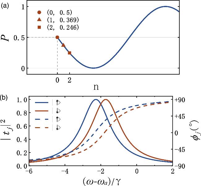


Figure 2. (a) The probability P(n) of finding spin state ∣ ↓ ⟩, with $n=\left\langle {c}^{\dagger }c\right\rangle $ being the photon number of inputting microwave. The figure is limited within so-called slope regime [3], i.e., ωs3t = (k + 1)π with k = 104, and thereby ωsct = (k + 1)πωsc/ωs3 ≈ 0.27π, with ωsc/2π ≈ 0.17MHz and ωs3/2π ≈ 6.394 GHz, as given by table 1. (b) Spin-dependent transmission spectrum (solid lines, left axis) and phase shift spectrum (dashed lines, right axis) of superconducting resonator. |
To experimentally detect the above probability P of the prepared spin superposition state, we use additional microwaves (referred to as detection waves) to probe the resonant frequency of the cavity. Let us consider the Hamiltonian of equation (8 ), wherein the last term shows that the cavity resonant frequency is spin-state dependent. Instead of the above weak signal wave, here the detection waves are sufficiently strong. Beyond the large-detuning, the real photon in cavity shall be excited in the present detection stage, as explained in Appendix B . Thus, the spin state can be detected by observing the transmission amplitude of the cavity [14, 23]. According to the well-known input-output theory [25, 26], the spin-dependent transmission amplitude of the cavity is expressed as $\hat{t}(\omega )$ = t1(ω)∣ ↓ ⟩⟨ ↓ ∣ +t2(ω)∣ ↑ ⟩⟨ ↑ ∣, with the component
$\begin{eqnarray}\begin{array}{r}{t}_{j}(\omega )=\frac{\gamma }{\gamma -{\rm{i}}[\omega -{\omega }_{a1}+{(-1)}^{j}{\omega }_{as}]}.\end{array}\end{eqnarray}$
and the line-width $\gamma =2\pi {g}_{ac}^{2}/{\omega }_{a}=2\pi \times 0.25\,{\rm{MHz}}$ [14]. The transmission amplitude tj is complex, wherein the ratio between the real and imaginary parts is solved as $\begin{eqnarray}\begin{array}{r}{\phi }_{j}(\omega )=\frac{\,\rm{Re}\,[{t}_{j}(\omega )]}{\,\rm{Im}\,[{t}_{j}(\omega )]}=\arctan \left[\frac{\omega -{\omega }_{a1}+{(-1)}^{j}{\omega }_{as}}{\gamma }\right].\end{array}\end{eqnarray}$
This ratio is usually called the phase shift of the transmission amplitude. Figure 2(b) shows the spin-dependent transmission probability ∣tj(ω)∣2 and the spin-dependent phase shift φj(ω), which can be used for precise measurements of the spin state. By performing repeated measurements of the spin state, the probability of the spin being in the down state can be determined, thus enabling the extraction of photon number information from figure 2(a).5. Conclusion
We have designed a micro-electrodes structure to trap a single surface-binding electron on liquid helium to couple it with the superconducting resonator. With the proposed electrode-circuit, we are able to load a dc current very close to the trapped electron for generating the strong spin–orbit coupling. Specifically, the lateral orbital vibration of trapped electron works within the GHz regime, and thus is strongly coupled to the usual superconducting resonators. At the same time, the orbital motion along the normal direction of helium surface is negligible throughout the paper, as its transition frequency is among the millimeter wave band.
With the help of the lateral spin–orbit coupling, the spin can be effectively manipulated by the electric dipole interaction in the microwave-driving cavity. Using the unitary transformation approach, we found an ac Stark effect of the trapped spin that is due to the external incoming microwave. In this process, both the electronic orbital state and the cavity photon are not excited. Therefore, without the strong decay occurring within the usual charge-qubits, the showed Stark effect of spin could be applied to implement the single photon detection of GHz microwave by using the famous Ramsey interferometry. Using again the spin–orbit coupling, the prepared Ramsey superposition state of spin can be detected by observing transmission amplitude of the superconducting resonator, as it has been already proposed by equation (14 ).
Appendix A The single qubit operation by spin–orbit coupling approach
We start with the Hamiltonian H0 given by our text, and apply a different microwave to drive the system. Under this driving, Hamiltonian H0 is extended to 4 ) and (6 ) as used by the text, the present Hamiltonian of equation (A1 ) can be approximately expressed as A2 ) reduces to HSQ2 = gscσy for a vacuum cavity in the ground state oscillator. As a consequence, the desired single qubit operation for spin is obtained,
$\begin{eqnarray}\begin{array}{r}{H}_{{\rm{SQ}}}={H}_{0}+\hslash {g}_{ac}({a}^{\dagger }{{\rm{e}}}^{-{\rm{i}}{\omega }_{d}t}+a{{\rm{e}}}^{+{\rm{i}}{\omega }_{d}t}).\end{array}\end{eqnarray}$
Similarly, applying unitary transformations equations ($\begin{eqnarray}\begin{array}{rcl}{H}_{{\rm{SQ1}}}/\hslash & \approx & {\omega }_{a1}{a}^{\dagger }a+{\omega }_{b1}{b}^{\dagger }b+\frac{1}{2}{\omega }_{s2}{\sigma }_{z}\\ & & -{\omega }_{as}{\sigma }_{z}{a}^{\dagger }a-{\omega }_{bs}{\sigma }_{z}{b}^{\dagger }b\\ & & +{g}_{ac}({a}^{\dagger }{{\rm{e}}}^{-{\rm{i}}{\omega }_{d}t}+a{{\rm{e}}}^{+{\rm{i}}{\omega }_{d}t})+{g}_{bc}({b}^{\dagger }{{\rm{e}}}^{-{\rm{i}}{\omega }_{d}t}\\ & & +b{{\rm{e}}}^{+{\rm{i}}{\omega }_{d}t})+{g}_{sc}({\sigma }_{+}{{\rm{e}}}^{-{\rm{i}}{\omega }_{d}t}+{\sigma }_{-}{{\rm{e}}}^{+{\rm{i}}{\omega }_{d}t}).\end{array}\end{eqnarray}$
In the rotating frame with frequency ωd, this Hamiltonian can be further written as [23]$\begin{eqnarray}\begin{array}{rcl}{H}_{{\rm{SQ2}}}/\hslash & \approx & ({\omega }_{a1}-{\omega }_{d}){a}^{\dagger }a+({\omega }_{b1}-{\omega }_{d}){b}^{\dagger }b\\ & & +{g}_{ac}({a}^{\dagger }+a)+{g}_{bc}({b}^{\dagger }+b)\\ & & +\frac{1}{2}({\omega }_{s2}-2{\omega }_{as}{a}^{\dagger }a-2{\omega }_{bs}{b}^{\dagger }b-{\omega }_{d}){\sigma }_{z}+{g}_{sc}{\sigma }_{y}.\end{array}\end{eqnarray}$
By setting gac ≪ ωa1 − ωd, gbc ≪ ωb1 − ωd, and ωs2 − ωd = 0, then the Hamiltonian of equation ($\begin{eqnarray}\begin{array}{rcl}{U}_{{\rm{SQ}}}({g}_{sc}t) & = & \exp \left(-{\rm{i}}{g}_{sc}t{\sigma }_{y}\right)\\ & = & \left(\begin{array}{cc}\cos {g}_{sc}t & -{\rm{i}}\sin {g}_{sc}t\\ -{\rm{i}}\sin {g}_{sc}t & \cos {g}_{sc}t\end{array}\right).\end{array}\end{eqnarray}$
Appendix B The input-output theory for spin state readout
Under the driving of continuous waves (inputting from one side of the cavity), the Hamiltonian of the spin-cavity system can be expressed as 4 ) and (6 ) mentioned by the text, we have the following effective Hamiltonian for (B1 ), B2 ) refer to the large-detuning drivings and are still negligible [24]. Thereby,
$\begin{eqnarray}\begin{array}{rcl}{H}_{{\rm{R}}} & = & {H}_{0}+{\displaystyle \int }_{-\infty }^{+\infty }{\rm{d}}\omega \hslash \omega {c}^{\dagger }(\omega )c(\omega )\\ & & +{\rm{i}}{\displaystyle \int }_{-\infty }^{+\infty }{\rm{d}}\omega \hslash {p}_{ac}\left[a{c}^{\dagger }(\omega )-c(\omega ){a}^{\dagger }\right].\end{array}\end{eqnarray}$
Here, ${p}_{ac}(\omega )\approx {p}_{ac}={g}_{ac}/\sqrt{{\omega }_{a}}$ describes the coupling strength between the inputting microwaves and the cavity field [22]. Again, using the unitary transformations equations ($\begin{eqnarray}\begin{array}{rcl}{H}_{{\rm{R1}}}/\hslash & \approx & ({\omega }_{a1}-{\omega }_{as}{\sigma }_{z}){a}^{\dagger }a+({\omega }_{b1}-{\omega }_{bs}{\sigma }_{z}){b}^{\dagger }b\\ & & +\frac{1}{2}{\omega }_{s2}{\sigma }_{z}+{\displaystyle \int }_{-\infty }^{+\infty }{\rm{d}}\omega \omega {c}^{\dagger }(\omega )c(\omega )\\ & & +{\rm{i}}{\displaystyle \int }_{-\infty }^{+\infty }{\rm{d}}\omega {p}_{ac}\left[a{c}^{\dagger }(\omega )-c(\omega ){a}^{\dagger }\right]\\ & & +{\rm{i}}{\displaystyle \int }_{-\infty }^{+\infty }{\rm{d}}\omega {p}_{bc}\left[b{c}^{\dagger }(\omega )-c(\omega ){b}^{\dagger }\right]\\ & & +{\rm{i}}{\displaystyle \int }_{-\infty }^{+\infty }{\rm{d}}\omega {p}_{sc}\left[{c}^{\dagger }(\omega ){\sigma }_{-}-c(\omega ){\sigma }_{+}\right].\end{array}\end{eqnarray}$
Here, ${p}_{bc}={g}_{bc}/\sqrt{{\omega }_{a}}$ and ${p}_{sc}={g}_{sc}/\sqrt{{\omega }_{a}}$. For some frequencies of the inputting waves, the last two terms in the above equation ($\begin{eqnarray}\begin{array}{rcl}{H}_{{\rm{R1}}}/\hslash & \approx & ({\omega }_{a1}-{\omega }_{as}{\sigma }_{z}){a}^{\dagger }a+\frac{1}{2}{\omega }_{s2}{\sigma }_{z}\\ & & +{\displaystyle \int }_{-\infty }^{+\infty }{\rm{d}}\omega \omega {c}^{\dagger }(\omega )c(\omega )\\ & & +{\rm{i}}{\displaystyle \int }_{-\infty }^{+\infty }{\rm{d}}\omega {p}_{ac}\left[a{c}^{\dagger }(\omega )-c(\omega ){a}^{\dagger }\right].\end{array}\end{eqnarray}$
As a consequence, the Heisenberg equations read $\begin{eqnarray}\begin{array}{r}\dot{{\sigma }_{z}}=0,\end{array}\end{eqnarray}$
$\begin{eqnarray}\begin{array}{r}\dot{c}(\omega )=-{\rm{i}}\omega c(\omega )+{p}_{ac}a(t),\end{array}\end{eqnarray}$
$\begin{eqnarray}\begin{array}{r}\dot{a}(t)=-{\rm{i}}({\omega }_{a1}-{\omega }_{as}{\sigma }_{z})a(t)-{\displaystyle \int }_{-\infty }^{+\infty }{\rm{d}}\omega {p}_{ac}c(\omega ).\end{array}\end{eqnarray}$
The solutions of equation (B5 ) can be formally written as B7 ) and equation (B8 ) into equation (B6 ), we have B9 ), we have
$\begin{eqnarray}\begin{array}{rcl}c\left(\omega ,t\gt {t}_{0}\right) & = & c\left(\omega ,t={t}_{0}\right){{\rm{e}}}^{-{\rm{i}}\omega \left(t-{t}_{0}\right)}\\ & & +{p}_{ac}{\displaystyle \int }_{{t}_{0}}^{t}a(t){{\rm{e}}}^{-{\rm{i}}\omega \left(t-t^{\prime} \right)}{\rm{d}}t^{\prime} ,\end{array}\end{eqnarray}$
and $\begin{eqnarray}\begin{array}{rcl}c\left(\omega ,t\lt {t}_{1}\right) & = & c\left(\omega ,t={t}_{1}\right){{\rm{e}}}^{-{\rm{i}}\omega \left(t-{t}_{1}\right)}\\ & & -{p}_{ac}{\displaystyle \int }_{t}^{{t}_{1}}a(t){{\rm{e}}}^{-{\rm{i}}\omega \left(t-t^{\prime} \right)}{\rm{d}}t^{\prime} .\end{array}\end{eqnarray}$
Substituting ($\begin{eqnarray}\begin{array}{rcl}\dot{a}(t) & = & -{\rm{i}}({\omega }_{a1}-{\omega }_{as}{\sigma }_{z})a(t)+\sqrt{\gamma }{a}_{{\rm{in}}}(t)-\frac{\gamma }{2}a(t),\\ \dot{a}(t) & = & -{\rm{i}}({\omega }_{a1}-{\omega }_{as}{\sigma }_{z})a(t)-\sqrt{\gamma }{a}_{{\rm{out}}}(t)+\frac{\gamma }{2}a(t),\end{array}\end{eqnarray}$
with $\gamma =2\pi {p}_{ac}^{2}$, and the so-called input-output operators: $\begin{eqnarray}\begin{array}{rcl}{a}_{{\rm{in}}}(t) & = & -\frac{1}{\sqrt{2\pi }}{\displaystyle \int }_{-\infty }^{+\infty }c(\omega ,t={t}_{0}){{\rm{e}}}^{-{\rm{i}}\omega (t-{t}_{0})}{\rm{d}}\omega ,\\ {a}_{{\rm{out}}}(t) & = & \frac{1}{\sqrt{2\pi }}{\displaystyle \int }_{-\infty }^{+\infty }c(\omega ,t={t}_{1}){{\rm{e}}}^{-{\rm{i}}\omega (t-{t}_{1})}{\rm{d}}\omega .\end{array}\end{eqnarray}$
Applying Fourier transforms to equation ($\begin{eqnarray}\begin{array}{rcl}-{\rm{i}}\omega a(\omega ) & = & -{\rm{i}}({\omega }_{a1}-{\omega }_{as}{\sigma }_{z})a(\omega )+\sqrt{\gamma }{a}_{{\rm{in}}}(\omega )-\frac{\gamma }{2}a(\omega ),\\ -{\rm{i}}\omega a(\omega ) & = & -{\rm{i}}({\omega }_{a1}-{\omega }_{as}{\sigma }_{z})a(\omega )-\sqrt{\gamma }{a}_{{\rm{out}}}(\omega )+\frac{\gamma }{2}a(\omega ),\end{array}\end{eqnarray}$
and consequently, the input-output relationship [24, 27, 28], $\begin{eqnarray}\begin{array}{r}{a}_{{\rm{in}}}(\omega )+{a}_{{\rm{out}}}(\omega )=\sqrt{\gamma }a(\omega ).\end{array}\end{eqnarray}$
Considering a two-side cavity, since the decay rate γ is associated with the left and right directions of the cavity, we distinguish it as γL and γR to represent the decay coefficients for the left and right cavities, respectively. Therefore, equation (B11 ) is modified as follows: B14 ), it follows that B17 ) can be expressed as
$\begin{eqnarray}\begin{array}{rcl}-{\rm{i}}\omega a(\omega ) & = & -{\rm{i}}({\omega }_{a1}-{\omega }_{as}{\sigma }_{z})a(\omega )+\sqrt{{\gamma }_{{\rm{L}}}}{a}_{{\rm{in}}}^{{\rm{L}}}(\omega )\\ & & -\frac{{\gamma }_{{\rm{L}}}}{2}a(\omega )+\sqrt{{\gamma }_{{\rm{R}}}}{a}_{{\rm{in}}}^{{\rm{R}}}(\omega )-\frac{{\gamma }_{{\rm{R}}}}{2}a(\omega ),\\ -{\rm{i}}\omega a(\omega ) & = & -{\rm{i}}({\omega }_{a1}-{\omega }_{as}{\sigma }_{z})a(\omega )-\sqrt{{\gamma }_{{\rm{L}}}}{a}_{{\rm{out}}}^{{\rm{L}}}(\omega )\\ & & +\frac{{\gamma }_{{\rm{L}}}}{2}a(\omega )-\sqrt{{\gamma }_{{\rm{R}}}}{a}_{{\rm{out}}}^{{\rm{R}}}(\omega )+\frac{{\gamma }_{{\rm{R}}}}{2}a(\omega ).\end{array}\end{eqnarray}$
And the above input-output relationship results in $\begin{eqnarray}\begin{array}{rcl}{a}_{{\rm{in}}}^{{\rm{L}}}(\omega )+{a}_{{\rm{out}}}^{{\rm{L}}}(\omega ) & = & \sqrt{{\gamma }_{{\rm{L}}}}a(\omega ),\\ {a}_{{\rm{in}}}^{{\rm{R}}}(\omega )+{a}_{{\rm{out}}}^{{\rm{R}}}(\omega ) & = & \sqrt{{\gamma }_{{\rm{R}}}}a(\omega ),\end{array}\end{eqnarray}$
Where ${a}_{{\rm{in}}}^{{\rm{L}}}({a}_{{\rm{in}}}^{{\rm{R}}})$ and ${a}_{{\rm{out}}}^{{\rm{L}}}({a}_{{\rm{out}}}^{{\rm{R}}})$ are respectively the input and output operators on the left (right) side of the cavity. Approximately, γL = γR = γ and consider the unilateral input of the cavity, i.e., ${a}_{{\rm{in}}}^{{\rm{R}}}=0$, the relationship between operators ${a}_{{\rm{in}}}^{{\rm{L}}}(\omega )$ and a(ω) can be derived as $\begin{eqnarray}\begin{array}{r}{a}_{{\rm{in}}}^{{\rm{L}}}(\omega )=\frac{\gamma +{\rm{i}}({\omega }_{a1}-{\omega }_{as}{\sigma }_{z})-{\rm{i}}\omega }{\sqrt{\gamma }}a(\omega ),\end{array}\end{eqnarray}$
and from the second line of equation ($\begin{eqnarray}\begin{array}{r}{a}_{{\rm{out}}}^{{\rm{R}}}(\omega )=\sqrt{\gamma }a(\omega ).\end{array}\end{eqnarray}$
Thus, we can obtain the explicit form of the spin-dependent transmission amplitude $\begin{eqnarray}\begin{array}{r}\hat{t}(\omega )=\frac{\langle {a}_{{\rm{out}}}^{{\rm{R}}}\rangle }{\langle {a}_{{\rm{in}}}^{{\rm{L}}}\rangle }=\frac{\langle \gamma a(\omega )\rangle }{\langle [\gamma -{\rm{i}}(\omega -{\omega }_{a1}+{\omega }_{as}{\sigma }_{z})]a(\omega )\rangle },\end{array}\end{eqnarray}$
Due to the presence of the operator σz, the spin-dependent transmission amplitude varies depending on the spin state. Considering both the spin-up and spin-down states of the electron, equation ($\begin{eqnarray}\begin{array}{r}\hat{t}(\omega )={t}_{1}(\omega )| \downarrow \rangle \langle \downarrow | +{t}_{2}(\omega )| \uparrow \rangle \langle \uparrow | ,\end{array}\end{eqnarray}$
with the component $\begin{eqnarray}\begin{array}{r}{t}_{j}(\omega )=\frac{\gamma }{\gamma -{\rm{i}}[\omega -{\omega }_{a1}+{(-1)}^{j}{\omega }_{as}]}.\end{array}\end{eqnarray}$
The phase factor is then simply derived by calculating the ratio of the real part to the imaginary part of the spin-dependent transmission amplitude, as shown below: $\begin{eqnarray}\begin{array}{rcl}{\phi }_{j}(\omega ) & = & \frac{\,\rm{Re}\,[{t}_{j}(\omega )]}{\,\rm{Im}\,[{t}_{j}(\omega )]}\\ & = & \arctan \left[\frac{\omega -{\omega }_{a1}+{(-1)}^{j}{\omega }_{as}}{\gamma }\right].\end{array}\end{eqnarray}$