

1. Introduction
‘Rogue waves' are special waves that exist for a very short period of time with extremely high wave heights, and there are no signs before their appearance [1]. For example, a large wave up to several tens of meters suddenly appears on a relatively calm sea surface. Oceanographers have been observing and studying rogue waves since the 1970s, and more and more scholars have begun to pay attention to this physical phenomenon, seeking explanations for rogue waves from both theoretical approaches and numerical simulations [2]. Peregrine, an expert in fluid mechanics, has obtained the rogue wave solution for the first time, for the nonlinear Schrödinger (NLS) equation, in terms of a rational function [3]. Subsequently, Akhmediev conducted a comprehensive analysis of the rogue waves for the NLS equation [4]. Rogue waves have always been an important research topic in integrable systems, and so far, there is no exact definition. In statistics, anomalous factors (${H}_{{\rm{Max}}}/{H}_{s}\gt 2$, ${H}_{{\rm{Max}}}$: the maximum wave height; Hs: the significant wave height, which means arranging a column of waves in ascending order and taking the average of the top one-third wave heights) are used to define rogue waves, widely accepted by many mathematicians [5]. The main characteristics of rogue waves is that these extreme waves ‘appear from nowhere and disappear without a trace' [6]. The rogue wave waveforms can be represented by quasi-rational solutions of the governing nonlinear evolution equations. Although rogue waves originated in the ocean, with the update of modern equipment and the improvement of technological means, the theory of rogue waves has also rapidly developed. A major driving force comes from the optical rogue waves observed in 2007 [7], which have since been widely applied in optics and photonics [8–11], plasma physics [12, 13], Bose–Einstein condensation [14–16], artificial neural networks [17], atmospheric physics, and superfluids [18, 19]. The main methods for constructing rogue waves include the bilinear method [20–22], the Kadomtsev–Petviashvili (KP) hierarchy reduction method, the Darboux transformation method, the inverse scattering transformation, the Lie group analysis [23–25], etc. The rogue wave solutions in one-dimensional systems are localized in both time and space, and their patterns mainly include eye shaped, inverse eye shaped, and distorted bimodal shapes [26–31]. The rogue waves in high-dimensional systems [32, 33] often appear in the form of line rogue waves, which are only localized in time and nonlocalized in space [34, 35]. Naturally, people expect to extend the properties of rogue wave solutions in low dimensional systems to high-dimensional systems from a mathematical perspective. From a practical application perspective, real ocean rogue waves exist on a two-dimensional plane, indicating the necessity of studying high-dimensional systems. Therefore, the construction and properties of time and space localized rogue wave solutions (doubly localized rogue wave solutions) in high-dimensional systems have always been a frontier and an important topic of great interest to researchers. There have been reported many meaningful results in this area [36–43] and the corresponding rogue wave solutions having standard symmetric shapes. However, rogue waves in the ocean have asymmetric shapes. Therefore, studying the asymmetric doubly localized rogue waves in integrable systems is of greater practical significance.
The nonlinear evolution equations can be divided into local and nonlocal ones, and the equations that people usually study are local ones. A few decades ago, Bender and Boettcher [44, 45] proposed the concept of space-time reflection symmetry, also known as parity-time (PT) symmetry in quantum mechanics. Their results indicate that as long as PT symmetry is not broken, the spectra of non-Hermitian Hamiltonian operators are real [44], whereas previously it was believed that only the spectra of Hermitian Hamiltonian operators were real. Inspired by those groundbreaking works, PT symmetry has not only made significant breakthroughs in theoretical and experimental physics [46–48], but also driven new developments in quantum field theory [49], optics and photonics [50, 51], Lie algebra [52], and complex crystals [53, 54]. The PT symmetry has important applications and extensions in many branches of natural sciences, and combining the PT symmetry with soliton theory became very natural. Ablowitz and Musslimani proposed a nonlocal NLS equation [55]
$\begin{eqnarray}{\rm{i}}{u}_{t}(x,t)-{u}_{xx}(x,t)-{u}^{2}(x,t){u}^{* }(-x,t)=0,\end{eqnarray}$
which is an extension of NLS equation that satisfies the PT symmetry condition. The multiple soliton solutions of nonlocal NLS equation were obtained using the inverse scattering method [55]. Then, various nonlinear waves of nonlocal NLS equation have been extensively studied [56–63]. Subsequently, several extended one-dimensional and two-dimensional nonlocal nonlinear evolution equations (NLEEs) were introduced, such as nonlocal vector type NLS equation [64, 65], nonlocal coupled NLS equation [66, 67], nonlocal sine-Gorden equation [68], nonlocal Davey–Stewartson (DS) equation [68, 69], nonlocal (2 + 1)-dimensional NLS equation [70, 71], nonlocal Mel'nikov equation [72, 73], nonlocal Sasa–Satsuma equation [74, 75], etc. These nonlocal systems are all complex one. An obvious and meaningful research direction is to construct real multidimensional integrable models with PT symmetry properties, and explore the generation mechanism and long-term asymptotic behavior of asymmetric doubly localized rogue waves.Based on the celebrated KP equation [76]2 ), we get 5 ).
$\begin{eqnarray}{({u}_{t}+\alpha u{u}_{x}+\beta {u}_{xxx})}_{x}+\gamma {u}_{yy}=0,\end{eqnarray}$
using the definition of the Alice-Bob operator proposed by Lou [77–79], and substituting $u=\frac{A+B}{2}$ into equation ( $\begin{eqnarray}\begin{array}{l}{A}_{xt}+{B}_{xt}+\frac{\alpha }{2}{({A}_{x}+{B}_{x})}^{2}\\ \,+\,\frac{\alpha }{2}(A+B)({A}_{xx}+{B}_{xx})+\beta ({A}_{xxxx}+{B}_{xxxx})\\ \,+\,\gamma ({A}_{yy}+{B}_{yy})=0.\end{array}\end{eqnarray}$
The following coupled equations can be derived $\begin{eqnarray}\begin{array}{l}{A}_{xt}+\frac{\alpha }{4}{({A}_{x}+{B}_{x})}^{2}+\frac{\alpha }{4}(A+B)({A}_{xx}+{B}_{xx})\\ \,+\,\beta {A}_{xxxx}+\gamma {A}_{yy}+G(A,B)=0,\\ {B}_{xt}+\frac{\alpha }{4}{({A}_{x}+{B}_{x})}^{2}+\frac{\alpha }{4}(A+B)({A}_{xx}+{B}_{xx})\\ \,+\,\beta {B}_{xxxx}+\gamma {B}_{yy}-G(A,B)=0,\end{array}\end{eqnarray}$
where B involves A through $B={\widehat{P}}_{s}^{x}{\widehat{P}}_{s}^{y}{\widehat{T}}_{d}\,A=A(-x,-y,-t)$ $({\widehat{P}}_{s}^{x}{\widehat{P}}_{s}^{y}{\widehat{T}}_{d}$ means the shifts of the space variables x and y to −x and −y, accompanied by the time reversal). G(A, B) is the function of A and B, and $G(A,B)={\widehat{P}}_{s}^{x}{\widehat{P}}_{s}^{y}{\widehat{T}}_{d}G(A,B)$. Specially, taking $G(A,B)\,=\,\frac{\alpha }{2}({A}_{x}^{2}+A{A}_{xx}-{B}_{x}^{2}-B{B}_{xx})$ the following nonlocal KP equation is introduced [80] $\begin{eqnarray}\begin{array}{l}{A}_{xt}+\frac{\alpha }{4}({A}_{x}+{B}_{x})(3{A}_{x}-{B}_{x})+\frac{\alpha }{4}(A-B){B}_{xx}\\ \,+\,\frac{\alpha }{4}(3A+B){A}_{xx}+\beta {A}_{xxxx}+\gamma {A}_{yy}=0,\\ B={\widehat{P}}_{s}^{x}{\widehat{P}}_{s}^{y}{\widehat{T}}_{d}A=A(-x,-y,-t).\end{array}\end{eqnarray}$
Although the soliton solutions, breather solutions, lump, ripple solutions of the nonlocal KP equation have been previously obtained [77–85], the semi-rational solutions formed by resonant collisions were not reported, to the best of our knowledge. In this paper, we mainly study the generation mechanism and long-term asymptotic behaviors of these resonant collision solutions for the nonlocal KP equation (2. The partial resonant collisions between solitons and lump waves
In this section, a family of semi-rational solutions of nonlocal KP equation (5 ) are presented by the partly resonant collisions between solitons and lump waves. These semi-rational solutions describe the interaction between multiple lumps and one soliton or multiple solitons, where the lump waves are semi-localized in time. In order to construct the target solutions, we must obtain the bilinear form of the nonlocal KP equation. The nonlocal KP equation (5 ) admits the bilinear form 6 ) of the nonlocal KP equation (5 ) can be reduced to the following bilinear equation of the KP hierarchy 8 ) admits the solutions 10 ) are selected as follows 6 ) reduces to the equation (8 ), and the tau functions are transformed into the corresponding solutions of the nonlocal KP equation (5 ). Thus, the semi-rational solutions of the nonlocal KP equation (5 ) can be written as the following Theorem.
$\begin{eqnarray}({D}_{x}{D}_{t}+\beta {D}_{x}^{4}+\gamma {D}_{y}^{2})f\cdot f=0,\end{eqnarray}$
using the transformations $\begin{eqnarray}\begin{array}{l}A=\frac{12\beta }{\alpha }{(\mathrm{ln}f)}_{xx}+{b}_{1}{(\mathrm{ln}f)}_{xxt}+{b}_{2}{(\mathrm{ln}f)}_{xxy},\\ B=\frac{12\beta }{\alpha }{(\mathrm{ln}f)}_{xx}-{b}_{1}{(\mathrm{ln}f)}_{xxt}-{b}_{2}{(\mathrm{ln}f)}_{xxy},\end{array}\end{eqnarray}$
where b1 and b2 are arbitrary constants, D is Hirota's bilinear differential operator [20]. The bilinear equation ( $\begin{eqnarray}[{D}_{{z}_{1}}^{4}-4{D}_{{z}_{1}}{D}_{{z}_{3}}+3{D}_{{z}_{2}}^{2}]{\tau }_{n}\cdot {\tau }_{n}=0.\end{eqnarray}$
The bilinear equation of KP hierarchy ( $\begin{eqnarray}\begin{array}{c}{\tau }_{n}=\mathop{\det }\limits_{1\leqslant {\rm{i}},j\leqslant N}({m}_{{\rm{i}},j}^{(n)}),\end{array}\end{eqnarray}$
and the matrix element ${m}_{{\rm{i}},j}^{(n)}$ satisfies $\begin{eqnarray}\begin{array}{l}{\partial }_{{z}_{1}}{m}_{{\rm{i}},j}^{(n)}={\varphi }_{{\rm{i}}}^{(n)}{\psi }_{j}^{(n)},\\ {m}_{{\rm{i}},j}^{(n+1)}={m}_{{\rm{i}},j}^{(n)}+{\varphi }_{{\rm{i}}}^{(n)}{\psi }_{j}^{(n+1)},\\ {\partial }_{{z}_{2}}{m}_{{\rm{i}},j}^{(n)}={\varphi }_{{\rm{i}}}^{(n+1)}{\psi }_{j}^{(n)}+{\varphi }_{{\rm{i}}}^{(n)}{\psi }_{j}^{(n-1)},\\ {\partial }_{{z}_{3}}{m}_{{\rm{i}},j}^{(n)}={\varphi }_{{\rm{i}}}^{(n+2)}{\psi }_{j}^{(n)}+{\varphi }_{{\rm{i}}}^{(n+1)}{\psi }_{j}^{(n-1)}+{\varphi }_{{\rm{i}}}^{(n)}{\psi }_{j}^{(n-2)},\\ {\partial }_{{z}_{k}}\varphi ={\varphi }_{{\rm{i}}}^{(n+k)},\quad {\partial }_{{z}_{k}}{\psi }_{{\rm{i}}}\\ \,=\,-{\psi }_{{\rm{i}}}^{(n-k)},(k=1,2,3).\end{array}\end{eqnarray}$
Here ${m}_{{\rm{i}},j}^{(n)}$, ${\varphi }_{{\rm{i}}}^{(n)}$, and ${\psi }_{j}^{(n)}$ are functions of the variables z1, z2, and z3. In order to construct the semi-rational solutions formed by the resonant collisions of lumps and solitons, the following differential operators are introduced $\begin{eqnarray}\begin{array}{l}{{\rm{\Xi }}}_{s}=\displaystyle \sum _{k=0}^{{n}_{s}}{a}_{sk}{({p}_{{\rm{i}}}{\partial }_{{p}_{s}})}^{{n}_{s}-k},\\ {\mho }_{j}=\displaystyle \sum _{l=0}^{{n}_{j}}{a}_{jl}^{* }{({p}_{j}^{\ast }{\partial }_{{p}_{j}^{\ast }})}^{{n}_{j}-l},\end{array}\end{eqnarray}$
and the functions ${m}_{s,j}^{(n)}$, ${\varphi }_{s}^{(n)}$, and ${\psi }_{j}^{(n)}$ in equation ( $\begin{eqnarray}\begin{array}{l}{\varphi }_{s}^{(n)}={{\rm{\Xi }}}_{s}{p}_{s}^{n}{{\rm{e}}}^{{\xi }^{s}},\\ {\psi }_{j}^{(n)}={\mho }_{j}{(-{q}_{j})}^{-n}{{\rm{e}}}^{{\eta }_{j}},\\ {m}_{s,j}^{(n)}={{\rm{\Xi }}}_{s}{\mho }_{j}\frac{1}{{p}_{s}+{p}_{j}^{\ast }}[{\delta }_{sj}+{\left(-\frac{{p}_{s}}{{p}_{j}^{\ast }}\right)}^{n}{{\rm{e}}}^{{\xi }_{s}+{\xi }_{j}^{* }}].\end{array}\end{eqnarray}$
For simplicity, the matrix elements ${m}_{s,j}^{(n)}$ are rewritten as $\begin{eqnarray}\begin{array}{l}{m}_{s,j}^{(n)}={\left(-\frac{{p}_{s}}{{p}_{j}^{\ast }}\right)}^{n}\,{{\rm{e}}}^{{\xi }_{s}+{\xi }_{j}^{* }}\displaystyle \sum _{k=0}^{{n}_{s}}{a}_{sk}\\ \,\times \,{({p}_{s}{\partial }_{{p}_{s}}+{\xi }_{s}^{{\prime} }+n)}^{{n}_{s}-k}\\ \,\times \,\displaystyle \sum _{l=0}^{{n}_{j}}{a}_{jl}^{* }{({p}_{j}^{* }{\partial }_{{p}_{j}^{* }}+{\xi }_{j}^{{}^{{\prime} }* }-n)}^{{n}_{j}-l}\\ \,\times \,\frac{1}{{p}_{s}+{p}_{j}^{* }}+{\delta }_{sj}{a}_{s{n}_{s}}{a}_{j{n}_{j}}^{* },\end{array}\end{eqnarray}$
where $\begin{eqnarray}\begin{array}{l}{\xi }_{s}={p}_{s}{z}_{1}+{p}_{s}^{2}{z}_{2}+{p}_{s}^{3}{z}_{3}+{\xi }_{s0},\\ {\xi }_{s}^{{\prime} }={p}_{s}{z}_{1}+2{p}_{s}^{2}{z}_{2}+3{p}_{s}^{3}{z}_{3}.\end{array}\end{eqnarray}$
Here δsj = 0, 1, ps and ask are complex constants, and ns are positive integers. Furthermore, taking the independent transformations $\begin{eqnarray}\begin{array}{l}{z}_{1}=\frac{1}{\sqrt[4]{\beta }}x,\quad {z}_{2}={\rm{i}}\sqrt{-\frac{3}{\gamma }}y,\\ \quad {z}_{3}=-4\sqrt[4]{\beta }t,\quad {\tau }_{0}=f,\end{array}\end{eqnarray}$
the bilinear equation (The nonlocal KP equation (
$\begin{eqnarray}\begin{array}{l}A=\frac{12\beta }{\alpha }{(\mathrm{ln}f)}_{xx}+{b}_{1}{(\mathrm{ln}f)}_{xxt}+{b}_{2}{(\mathrm{ln}f)}_{xxy},\\ B=\frac{12\beta }{\alpha }{(\mathrm{ln}f)}_{xx}-{b}_{1}{(\mathrm{ln}f)}_{xxt}-{b}_{2}{(\mathrm{ln}f)}_{xxy},\end{array}\end{eqnarray}$
where $\begin{eqnarray}f=\mathop{\det }\limits_{1\,\leqslant \,s,j\,\leqslant \,N}({m}_{s,j}^{(0)}),\end{eqnarray}$
and the matrix elements are defined by $\begin{eqnarray}\begin{array}{l}{m}_{s,j}^{(n)}={\left(-\frac{{p}_{s}}{{p}_{j}^{\ast }}\right)}^{n}\,{{\rm{e}}}^{{\xi }_{s}+{\xi }_{j}^{* }}\displaystyle \sum _{k=0}^{{n}_{s}}{a}_{sk}{({p}_{s}{\partial }_{{p}_{s}}+{\xi }_{s}^{{\prime} }+n)}^{{n}_{s}-k}\\ \,\times \,\displaystyle \sum _{l=0}^{{n}_{j}}{a}_{jl}^{* }{({p}_{j}^{* }{\partial }_{{p}_{j}^{* }}+{\xi }_{j}^{{}^{{\prime} }* }-n)}^{{n}_{j}-l}\frac{1}{{p}_{s}+{p}_{j}^{* }}+{\alpha }_{sj},\end{array}\end{eqnarray}$
$\begin{eqnarray*}\begin{array}{l}{\xi }_{j}=\frac{1}{\sqrt[4]{\beta }}{p}_{j}x+{\rm{i}}\sqrt{-\frac{3}{\gamma }}{p}_{j}^{2}y-4\sqrt[4]{\beta }{p}_{j}^{3}t+{\xi }_{j0},\\ {\xi }_{j}^{{\prime} }=\frac{1}{\sqrt[4]{\beta }}{p}_{j}x+2{\rm{i}}\sqrt{-\frac{3}{\gamma }}{p}_{j}^{2}y-12\sqrt[4]{\beta }{p}_{j}^{3}t.\end{array}\end{eqnarray*}$
The asterisk denotes the complex conjugation, s, j, k, and l are arbitrary positive integers. The semi-rational solutions will reduce to the rational solutions as αsj = 0.
2.1. The partial resonant collisions between one lump wave and one soliton
Taking N = 1, ni = 1, in theorem 1, the fundamental semi-rational solutions A and B consisting of a lump wave and a soliton are obtained, 19 ) are lump waves as α11 = 0. From the evolution of the lump in figure 1, it can be seen that the waveform of the lump is symmetric when b1 = b2 = 0, otherwise it is asymmetric when b1b2 ≠ 0.
$\begin{eqnarray}\begin{array}{rcl}A & = & \frac{12\beta }{\alpha }{(\mathrm{ln}f)}_{xx}+{b}_{1}{(\mathrm{ln}f)}_{xxt}+{b}_{2}{(\mathrm{ln}f)}_{xxy},\\ B & = & \frac{12\beta }{\alpha }{(\mathrm{ln}f)}_{xx}-{b}_{1}{(\mathrm{ln}f)}_{xxt}-{b}_{2}{(\mathrm{ln}f)}_{xxy},\\ f & = & {{\rm{e}}}^{{\xi }_{1}+{\xi }_{1}^{* }}\displaystyle \sum _{k=0}^{1}{a}_{1k}{({\partial }_{{p}_{1}}+{\xi }_{1}^{{\prime} })}^{1-k}\\ & & \times \,\displaystyle \sum _{l=0}^{1}{a}_{1l}^{* }{({\partial }_{{p}_{1}^{\ast }}+{\xi }_{1}^{{}^{{\prime} }* })}^{1-l}\frac{1}{{p}_{1}+{p}_{1}^{\ast }}+{\alpha }_{11}\\ & = & {{\rm{e}}}^{{\xi }_{1}+{\xi }_{1}^{* }}({\partial }_{{p}_{1}}+{\xi }_{1}^{{\prime} }+{a}_{11})\\ & & \times \,({\partial }_{{p}_{1}^{\ast }}+{\xi }_{1}^{{}^{{\prime} }* }+{a}_{11}^{* })\frac{1}{{p}_{1}+{p}_{1}^{\ast }}+{\alpha }_{11}\\ & = & \frac{{{\rm{e}}}^{{\xi }_{1}+{\xi }_{1}^{* }}}{{p}_{1}+{p}_{1}^{\ast }}\left[\left({\xi }_{1}^{{\prime} }+{a}_{11}-\frac{1}{{p}_{1}+{p}_{1}^{\ast }}\right)\right.\\ & & \times \,\left.({\xi }_{1}^{{}^{{\prime} }* }+{a}_{11}^{* }-\frac{1}{{p}_{1}+{p}_{1}^{\ast }})+\frac{1}{{({p}_{1}+{p}_{1}^{\ast })}^{2}}\right]+{\alpha }_{11},\end{array}\end{eqnarray}$
with $\begin{eqnarray*}\begin{array}{l}{\xi }_{1}=\frac{1}{\sqrt[4]{\beta }}{p}_{1}x+{\rm{i}}\sqrt{-\frac{3}{\gamma }}{p}_{1}^{2}y-4\sqrt[4]{\beta }{p}_{1}^{3}t+{\xi }_{10},\\ {\xi }_{1}^{{\prime} }=\frac{1}{\sqrt[4]{\beta }}{p}_{1}x+2{\rm{i}}\sqrt{-\frac{3}{\gamma }}{p}_{1}^{2}y-12\sqrt[4]{\beta }{p}_{1}^{3}t,\end{array}\end{eqnarray*}$
where p1 and a11 are complex constants. Assuming α = 1, β = 1, γ = − 1, p1 = pR + ipI, a11 = aR + iaI, then the function f is rewritten as $\begin{eqnarray}f=\frac{{{\rm{e}}}^{{\xi }_{1}+{\xi }_{1}^{* }}}{2{p}_{R}}(\theta {\theta }^{* }+{\theta }_{0})+{\delta }_{11}({a}_{R}^{2}+{a}_{I}^{2}),\end{eqnarray}$
with $\begin{eqnarray*}\begin{array}{l}\theta ={L}_{1}+{\rm{i}}{L}_{2},{L}_{1}={p}_{R}x+4\sqrt{3}{p}_{R}y\\ \,+\,(36{p}_{R}{p}_{I}^{2}-12{p}_{R}^{3})t+{a}_{R}-\frac{1}{2{p}_{R}},\\ {\theta }_{0}=\frac{1}{4{p}_{R}^{2}},\,\,\qquad {L}_{2}={p}_{I}x+2\sqrt{3}({p}_{I}^{2}-{p}_{R}^{2})y\\ \,+\,(12{p}_{I}^{3}-36{p}_{R}^{2}{p}_{I})t+{a}_{I},\,\,\end{array}\end{eqnarray*}$
where pR, pI, aR, aI are real constants. The corresponding semi-rational solutions (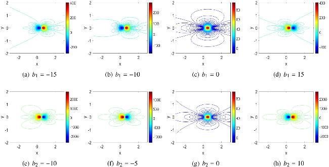
Figure 1. The evolution of one-lump on the constant background with parameters α = 1, β = 1, γ = −1, (a)–(d): p1 = 1, b2 = 0, α11 = 0, t = 0; (e)–(h): p1 = 1, b1 = 0, α11 = 0, t = 0. |
The corresponding semi-rational solutions (19 ) describe the resonant collision between one lump wave and one soliton as α11 ≠ 0. We further take α = 1, β = 1, γ = −1, p1 = 1, b1 = 0, b2 = 0. As shown in figure 2, there is no lump wave at t → −∞, but a lump wave suddenly arises from one soliton and propagates forward steadily with its own amplitude and velocity when t → +∞. In this case, the lump wave is semi-localized in time, and this collision is called a partial resonant collision. The lump has the following three extreme points 19 ), one maximum ${A}_{{\rm{Max}}}$ [the red line of planes (e)–(g) in figure 2] and two minimum values ${A}_{{\rm{Min}}-1}$ [the green line of planes (e)–(g) in figure 2] and ${A}_{{\rm{Min}}-2}$ [the blue line of planes (e)–(g) in figure 2] of the lump wave can be obtained
$\begin{eqnarray}\begin{array}{l}{l}_{1}(x,y)=\left(\frac{4}{3}t-\frac{3}{2},0\right),\\ {l}_{2}(x,y)=\left(\frac{4}{3}t-\frac{3}{2}+\frac{3\sqrt{3}}{2},0\right),\\ {l}_{3}(x,y)=\left(\frac{4}{3}t+\frac{3}{2}+\frac{3\sqrt{3}}{2},0\right).\end{array}\end{eqnarray}$
By substituting the above extreme points into equation ( $\begin{eqnarray}\begin{array}{l}{A}_{{\rm{Max}}}=A{| }_{{l}_{1}}=\frac{32{{\rm{\Lambda }}}_{1}}{27}\,\frac{2660{{\rm{\Lambda }}}_{1}-243{{\rm{\Lambda }}}_{1}^{2}+5792}{{(8+3{{\rm{\Lambda }}}_{1})}^{3}},\\ {A}_{{\rm{Min}}-1}=A{| }_{{l}_{2}}=-\frac{4{{\rm{\Lambda }}}_{2}}{81}\\ \,\times \,\frac{336\sqrt{3}{{\rm{\Lambda }}}_{2}+1410{{\rm{\Lambda }}}_{2}+729{{\rm{\Lambda }}}_{2}^{2}-2096\sqrt{3}-3384}{{(2+3{{\rm{\Lambda }}}_{2})}^{3}},\\ {A}_{{\rm{Min}}-2}=A{| }_{{l}_{3}}=\frac{4{{\rm{\Lambda }}}_{3}}{81}\\ \,\times \,\frac{336\sqrt{3}{{\rm{\Lambda }}}_{3}-1410{{\rm{\Lambda }}}_{3}-729{{\rm{\Lambda }}}_{3}^{2}-2096\sqrt{3}+3384}{{(2+3{{\rm{\Lambda }}}_{2})}^{3}},\\ {{\rm{\Lambda }}}_{1}={{\rm{e}}}^{\frac{16}{27}t-1},\quad {{\rm{\Lambda }}}_{2}={{\rm{e}}}^{\frac{16}{27}t-1+\sqrt{3}},\quad {{\rm{\Lambda }}}_{3}={{\rm{e}}}^{\frac{16}{27}t-1-\sqrt{3}}.\end{array}\end{eqnarray}$
The evolution of these maximum values can be seen in figures 2(e)–(g); the maximum value ${A}_{{\rm{Max}}}$ reaches 12.36, and the minimum value ${A}_{{\rm{Min}}-1}$ reaches 3.86. Moreover, these asymptotic behaviors [figures 2(e)–(g)] match the evolution of the three-dimensional plots [figures 2(a)–(d)].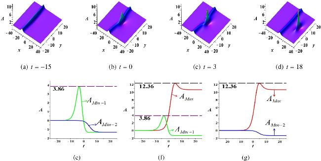
Figure 2. (a)–(d): The evolution of a lump on the background of one soliton with parameters α = 1, β = 1, γ = −1, p1 = 1, b1 = 0, b2 = 0, α11 = 1; (e)–(g): The evolution of the maximum ${A}_{{\rm{Max}}}$ [the red line] and two minimum values ${A}_{{\rm{Min}}-1}$ [the green line] and ${A}_{{\rm{Min}}-2}$ [the blue line] with parameters α = 1, β = 1, γ = −1, p1 = 1, b1 = 0, b2 = 0, α11 = 1. |
2.2. The partial resonant collisions between multiple lumps and one soliton
Taking N = 1, ni ≥ 2 in theorem 1, the semi-rational solutions generated by the resonance collision of multiple lump waves and one soliton are given. For example, we obtain the semi-rational solutions composed of two lumps and one soliton when N = 1, ni = 2, and their analytical expressions are as follows 18 ). Further, taking in equation (23 ) $\alpha =1,\beta =1,\gamma =-1,{\alpha }_{11}=0,{p}_{1}=\frac{1}{2},{a}_{12}=1$, the above function f can be rewritten as 24 ), when t → +∞ this solution achieves its maximum value of 24 at the following two coordinates
$\begin{eqnarray}\begin{array}{l}A=\frac{12\beta }{\alpha }{(\mathrm{ln}f)}_{xx}+{b}_{1}{(\mathrm{ln}f)}_{xxt}+{b}_{2}{(\mathrm{ln}f)}_{xxy},\\ B=\frac{12\beta }{\alpha }{(\mathrm{ln}f)}_{xx}-{b}_{1}{(\mathrm{ln}f)}_{xxt}-{b}_{2}{(\mathrm{ln}f)}_{xxy},\\ f={{\rm{e}}}^{{\xi }_{1}+{\xi }_{1}^{* }}[{({\partial }_{{p}_{1}}+{\xi }_{1}^{{\prime} })}^{2}+{a}_{12}][{({\partial }_{{p}_{1}^{\ast }}+{\xi }_{1}^{{}^{{\prime} }* })}^{2}+{a}_{12}^{* }]\\ \,\times \,\frac{1}{{p}_{1}+{p}_{1}^{* }}+{\alpha }_{11},\end{array}\end{eqnarray}$
where ξ1 is given in ( $\begin{eqnarray}\begin{array}{l}f=\frac{81}{16}{t}^{4}-\frac{27}{4}(x+2){t}^{3}+\frac{9}{8}(3{x}^{2}+3{y}^{2}+8x+14){t}^{2}\\ \,-\,\frac{3}{4}({x}^{3}+2{x}^{2}+3x{y}^{2}+6x+6)t\\ \,+\,\frac{1}{16}{x}^{4}+\frac{3}{8}({y}^{2}+2){x}^{2}+\frac{1}{2}(3{y}^{2}-1)x+\frac{9}{16}{y}^{4}+\frac{3}{2}.\end{array}\end{eqnarray}$
The corresponding solutions describe the dynamics of two lump waves with similar properties, as shown in figure 3. In this case, the trajectories of these two lump waves are as follows $\begin{eqnarray}\begin{array}{l}{L}_{1}:(x,y)\\ \,=\,\left(t-\frac{1}{6}-\frac{{w}_{1}}{6},\,\,\frac{\sqrt{2t{w}_{1}-24{t}^{2}-\frac{11}{6}{w}_{1}-4t+\frac{17}{6}}}{3}\right),\\ {L}_{2}:(x,y)\\ \,=\,\left(t-\frac{1}{6}-\frac{{w}_{1}}{6},\,\,-\frac{\sqrt{2t{w}_{1}-24{t}^{2}-\frac{11}{6}{w}_{1}-4t+\frac{17}{6}}}{3}\right),\\ {L}_{3}:(x,y)=\left({w}_{2}-\frac{2-4t}{{w}_{2}}+3t,\,\,0\right),\\ {w}_{1}={(114{t}^{2}-120t-11)}^{\frac{1}{2}},\\ {w}_{2}={\left(1+\sqrt{-64{t}^{3}+96{t}^{2}-48t+9}\right)}^{\frac{1}{3}}.\end{array}\end{eqnarray}$
In the case of equation ( $\begin{eqnarray}\begin{array}{l}\left(t-\frac{1}{6}-\frac{{w}_{1}}{6},\,\,\pm \frac{\sqrt{2t{w}_{1}-24{t}^{2}-\frac{11}{6}{w}_{1}-4t+\frac{17}{6}}}{3}\right),\\ {w}_{1}={(114{t}^{2}-120t-11)}^{\frac{1}{2}},\end{array}\end{eqnarray}$
and its minimum value −3 at the following four coordinates $\begin{eqnarray}\left(t-\frac{1}{6}-\frac{{w}_{1}}{6}\pm \sqrt{3},\,\,\pm \frac{\sqrt{2t{w}_{1}-24{t}^{2}-\frac{11}{6}{w}_{1}-4t+\frac{17}{6}}}{3}\right),\end{eqnarray}$
and the above equations have a good definition when $t\lt -\frac{1}{12}$.When t → −∞, this solution achieves its maximum value of 24 at the following two coordinates
$\begin{eqnarray}\left(\pm \left[{w}_{2}-\frac{2-4t}{{w}_{2}}\right]+3t,\,\,0\right),\end{eqnarray}$
and its minimum value −3 at the following four coordinates $\begin{eqnarray}\left(\pm \left[{w}_{2}-\frac{2-4t}{{w}_{2}}\right]+3t\pm \sqrt{3},\,\,0\right),\end{eqnarray}$
and the above equations have a good definition when $t\gt \frac{3}{4}$.Taking in equation (23 ) α11 = 1, the corresponding semi-rational solutions (23 ) describe the partial resonant collision of two lump waves and one soliton. As shown in figure 4, two lumps fission from one soliton. Finally, the two lumps and solitons are completely separated and maintain their respective waveforms during propagation. Clearly, these lumps are semi-localized in time and are a type of partial resonant collision.
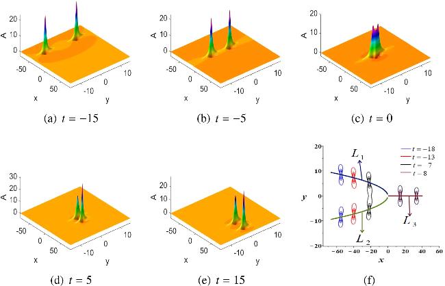
Figure 3. (a)–(e): The evolution of two lumps on the constant background with parameters α = 1, β = 1, γ = −1, ${p}_{1}=\frac{1}{2}$, b1 = 0, b2 = 0, α11 = 0; (f): the contour plots of the corresponding solution ( |
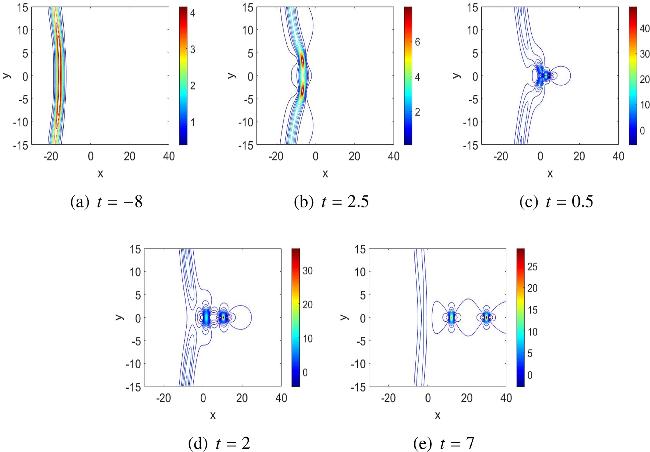
Figure 4. The evolution of two lumps on the soliton background with parameters $\alpha =1,\beta =1,\gamma =-1,{p}_{1}=\frac{1}{2},{b}_{1}=0,{b}_{2}=0,{\alpha }_{11}=1$. |
2.3. The partial resonant collisions between multi-lump waves and multiple solitons
Next, the partial resonant collision of multiple lumps and multiple solitons is considered. Taking N ≥ 2, ni = 1 in theorem 1, the semi-rational solutions generated by the partial resonance collision of N lump waves and N solitons are presented. These semi-rational solutions are formed by resonant collisions as these lump waves are semi-localized in time. For the choice N = 2, ni = 1, the corresponding solutions are written as 18 ). Further, taking in equation $\alpha =1,\beta =1,\gamma =-1,{p}_{1}=\frac{1}{3},{p}_{2}=\frac{1}{2},{\alpha }_{sj}=0$, the function f can be rewritten as
$\begin{eqnarray}\begin{array}{l}A=\frac{12\beta }{\alpha }{(\mathrm{ln}f)}_{xx}+{b}_{1}{(\mathrm{ln}f)}_{xxt}+{b}_{2}{(\mathrm{ln}f)}_{xxy},\\ B=\frac{12\beta }{\alpha }{(\mathrm{ln}f)}_{xx}-{b}_{1}{(\mathrm{ln}f)}_{xxt}-{b}_{2}{(\mathrm{ln}f)}_{xxy},\end{array}\end{eqnarray}$
with $\begin{eqnarray*}\begin{array}{l}f=\left|\begin{array}{cc}{K}_{11}^{(0)} & {K}_{12}^{(0)}\\ {K}_{21}^{(0)} & {K}_{22}^{(0)}\end{array}\right|,\,{K}_{sj}^{(0)}=\frac{{{\rm{e}}}^{{\xi }_{s}+{\xi }_{j}^{* }}}{{p}_{s}+{p}_{j}^{* }}\\ \,\times \,\left[({\xi }_{s}^{{\prime} }-\frac{1}{{p}_{s}+{p}_{j}^{* }}+{a}_{s1})({\xi }_{j}^{{}^{{\prime} }* }-\frac{1}{{p}_{s}+{p}_{j}^{* }}+{a}_{j1}^{* })+\frac{1}{{({p}_{s}+{p}_{j}^{* })}^{2}}\right]\\ \,+\,{\alpha }_{sj},\,\,s,j=1,2,\end{array}\end{eqnarray*}$
where ξs is given in ( $\begin{eqnarray*}\begin{array}{l}f=\left[\frac{1}{6}{\left(x-\frac{4}{3}t+\frac{3}{2}\right)}^{2}+\frac{2}{9}{y}^{2}+\frac{3}{8}\right]\\ \,\cdot \,\left[\frac{1}{4}{(x-3t+1)}^{2}+\frac{3}{4}{y}^{2}+\frac{1}{4}\right]\\ \,+\,\left[\frac{12}{225}{\left(t+\frac{1}{2}x+\frac{19}{10}\right)}^{2}\right]\\ \,-\,\left[\frac{4}{5}{\left(t-\frac{13}{24}x-\frac{97}{120}\right)}^{2}-\frac{5}{144}{\left(x+\frac{13}{5}\right)}^{2}+\frac{2}{5}{y}^{2}+\frac{36}{125}\right].\end{array}\end{eqnarray*}$
The corresponding solution describes the collision of two different types of lump waves, and their dynamics are different from figure 3. As shown in figure 5, the short and chubby lump wave is in front of the tall and thin lump wave at t ≪ −10. As time passes, the tall and thin lump wave catches up with the short and chubby lump wave, and the two lumps merge and split into two similar lump waves. These two similar lump waves fuse at extreme times and then split into the initial tall and thin lump wave and the short and chubby lump wave. Finally, the tall and thin lump wave is in front of the short and chubby lump wave at t ≫ 19.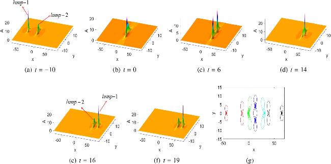
Figure 5. The evolution of two lumps on the constant background with parameters α = 1, β = 1, γ = −1, ${p}_{1}=\frac{1}{3}$, ${p}_{2}=\frac{1}{2}$, b1 = 0, b2 = 0, α11 = 0. (g): The contour plots of the corresponding solution ( |
Taking in equation $\alpha =1,\beta =1,\gamma =-1,{p}_{1}=\frac{1}{3},{p}_{2}=\frac{1}{2},{\alpha }_{sj}=0$, the corresponding solution describes the collision of two different types of lump waves and solitons. As seen in figure 6 two lump waves suddenly appear from two solitons and eventually propagate forward while maintaining their respective waveforms and velocities. The two lump waves are semi-localized in time and are a type of partial resonant collision.
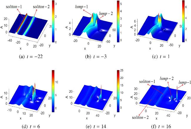
Figure 6. The evolution of two lumps on the two solitons background with parameters α = 1, β = 1, $\gamma =-1,{p}_{1}=\frac{1}{3}$, ${p}_{2}=\frac{1}{2},{b}_{1}=0,{b}_{2}=0$, α11 = 1. |
3. The full resonant collisions between solitons and lump waves
In this section, a family of semi-rational solutions of nonlocal KP equation (5 ) are presented by the full resonant collisions between solitons and lump waves, where the lump waves are localized in time and space. To construct the target solutions, the parameters in theorem 1 are restricted as 5 ) are given by the following theorem 2.
$\begin{eqnarray}\begin{array}{rcl}{p}_{s} & = & {p}_{j}=p,\,\,N=M+1,\\ {n}_{s} & = & M+1-s,\,\,{n}_{j}=M+1-j,\,\,{\xi }_{s0}=\overline{{\xi }_{s}},\\ {\xi }_{j0} & = & \overline{{\xi }_{j}},\end{array}\end{eqnarray}$
and the new semi-rational solutions of the nonlocal KP equation (The nonlocal KP equation (
$\begin{eqnarray}\begin{array}{l}A=\frac{12\beta }{\alpha }{(\mathrm{ln}{\tau }_{0})}_{xx}+{b}_{1}{(\mathrm{ln}{\tau }_{0})}_{xxt}+{b}_{2}{(\mathrm{ln}{\tau }_{0})}_{xxy},\\ B=\frac{12\beta }{\alpha }{(\mathrm{ln}{\tau }_{0})}_{xx}-{b}_{1}{(\mathrm{ln}{\tau }_{0})}_{xxt}-{b}_{2}{(\mathrm{ln}{\tau }_{0})}_{xxy},\end{array}\end{eqnarray}$
where ${\tau }_{n}={\left|{m}_{s,j}^{(n)}\right|}_{1\leqslant s,j\leqslant M+1}$ and the matrix elements are defined as $\begin{eqnarray}\begin{array}{l}{m}_{s,j}^{(n)}={\alpha }_{sj}+(-\frac{p}{{p}^{* }}){{\rm{e}}}^{\xi +{\xi }^{* }+\overline{{\xi }_{s}}+\overline{{\xi }_{j}^{* }}}\\ \,\times \,\displaystyle \sum _{k=0}^{M+1-s}{a}_{sk}{(p{\partial }_{p}+{\xi }^{{\prime} }+n)}^{M+1-s-k}\\ \,\times \,\displaystyle \sum _{l=0}^{M+1-j}{a}_{jl}^{* }{({p}^{* }{\partial }_{{p}^{* }}+{\xi }^{{}^{{\prime} }* }-n)}^{M+1-j-l}\frac{1}{p+{p}^{* }},\end{array}\end{eqnarray}$
with $\begin{eqnarray}\begin{array}{l}\xi =\frac{1}{\sqrt[4]{\beta }}px+{\rm{i}}\sqrt{-\frac{3}{\gamma }}{p}^{2}y-4\sqrt[4]{\beta }{p}^{3}t+{\xi }_{j0},\\ {\xi }^{{\prime} }=\frac{1}{\sqrt[4]{\beta }}px+2{\rm{i}}\sqrt{-\frac{3}{\gamma }}{p}^{2}y-12\sqrt[4]{\beta }{p}^{3}t,\end{array}\end{eqnarray}$
where s, j, k, and l are positive integers, λ and s are arbitrary real constants,and $p,\overline{{\xi }_{j}}$ are complex constants.3.1. The fundamental full resonant collisions between solitons and lump waves
The simplest case of full resonant collisions is first discussed, which matches the semi-rational solution in theorem 2 with M = 1. The fundamental full resonant collision solutions are as follows 5 ). In order to facilitate the analysis of the asymptotic behaviors of these solutions, the solutions A and B defined in (35 ) are rewritten as
$\begin{eqnarray}\begin{array}{l}A=\left(\frac{12\beta }{\alpha }{\partial }_{xx}+{b}_{1}{\partial }_{xxt}+{b}_{2}{\partial }_{xxy}\right)\,\,(\mathrm{ln}f),\\ B=\left(\frac{12\beta }{\alpha }{\partial }_{xx}-{b}_{1}{\partial }_{xxt}-{b}_{2}{\partial }_{xxy}\right)\,\,(\mathrm{ln}f),\end{array}\end{eqnarray}$
where $\begin{eqnarray}\begin{array}{l}f=1+\frac{1}{p+{p}^{* }}{{\rm{e}}}^{\xi +{\xi }^{* }+\overline{{\xi }_{1}}+\overline{{\xi }_{1}^{* }}}\left[{f}_{{\rm{r}}{\rm{a}}{\rm{t}}{\rm{i}}{\rm{o}}{\rm{n}}{\rm{a}}{\rm{l}}}+{{\rm{e}}}^{\overline{{\xi }_{2}}+\overline{{\xi }_{2}^{* }}-\overline{{\xi }_{1}}-\overline{{\xi }_{1}^{* }}}\right]\\ \,+\,\frac{p{p}^{* }}{{(p+{p}^{* })}^{4}}{{\rm{e}}}^{2(\xi +{\xi }^{* })+\overline{{\xi }_{2}}+\overline{{\xi }_{2}^{* }}+\overline{{\xi }_{1}}+\overline{{\xi }_{1}^{* }}},\end{array}\end{eqnarray}$
with $\begin{eqnarray}\begin{array}{rcl}{f}_{{\rm{r}}{\rm{a}}{\rm{t}}{\rm{i}}{\rm{o}}{\rm{n}}{\rm{a}}{\rm{l}}} & = & ({\xi }^{{\prime} }-\frac{p}{p+{p}^{* }})({\xi }^{{}^{{\prime} }* }-\frac{{p}^{* }}{p+{p}^{* }})\\ & & +\frac{p{p}^{* }}{{(p+{p}^{* })}^{2}}.\end{array}\end{eqnarray}$
Significantly, the functions $\begin{eqnarray}\begin{array}{l}\widetilde{A}=\left(\frac{12\beta }{\alpha }{\partial }_{xx}+{b}_{1}{\partial }_{xx{\rm{t}}}+{b}_{2}{\partial }_{xxy}\right)\,\,(\mathrm{ln}{f}_{{\rm{r}}{\rm{a}}{\rm{t}}{\rm{i}}{\rm{o}}{\rm{n}}{\rm{a}}{\rm{l}}}),\\ \widetilde{B}=\left(\frac{12\beta }{\alpha }{\partial }_{xx}-{b}_{1}{\partial }_{xx{\rm{t}}}-{b}_{2}{\partial }_{xxy}\right)\,\,(\mathrm{ln}{f}_{{\rm{r}}{\rm{a}}{\rm{t}}{\rm{i}}{\rm{o}}{\rm{n}}{\rm{a}}{\rm{l}}}),\end{array}\end{eqnarray}$
are the rational solutions of the nonlocal KP equation ( $\begin{eqnarray}\begin{array}{l}A=\left(\frac{12\beta }{\alpha }{\partial }_{xx}+{b}_{1}{\partial }_{xxt}+{b}_{2}{\partial }_{xxy}\right)\,\,(\mathrm{ln}\widehat{f}),\\ B=\left(\frac{12\beta }{\alpha }{\partial }_{xx}-{b}_{1}{\partial }_{xxt}-{b}_{2}{\partial }_{xxy}\right)\,\,(\mathrm{ln}\widehat{f}),\\ \widehat{f}={{\rm{e}}}^{-(\xi +{\xi }^{* }+\overline{{\xi }_{1}}+\overline{{\xi }_{1}^{* }})}+{{\rm{e}}}^{\widetilde{f}}+{{\rm{e}}}^{2(\xi +{\xi }^{* })+\overline{{\xi }_{2}}+\overline{{\xi }_{2}^{* }}+\overline{{\xi }_{1}}+\overline{{\xi }_{1}^{* }}+{\delta }_{0}},\\ \widehat{g}={{\rm{e}}}^{-(\xi +{\xi }^{* }+\overline{{\xi }_{1}}+\overline{{\xi }_{1}^{* }})-2{\rm{i}}{\delta }_{1}}+{{\rm{e}}}^{\widetilde{g}}\\ \,+\,{{\rm{e}}}^{2(\xi +{\xi }^{* })+\overline{{\xi }_{2}}+\overline{{\xi }_{2}^{* }}+\overline{{\xi }_{1}}+\overline{{\xi }_{1}^{* }}+{\delta }_{0}+2{\rm{i}}{\delta }_{1}},\end{array}\end{eqnarray}$
with $\begin{eqnarray}\widetilde{f}=\mathrm{ln}\left(\frac{{f}_{{\rm{r}}{\rm{a}}{\rm{t}}{\rm{i}}{\rm{o}}{\rm{n}}{\rm{a}}{\rm{l}}}+{{\rm{e}}}^{\overline{{\xi }_{2}}+\overline{{\xi }_{2}^{* }}-\overline{{\xi }_{1}}-\overline{{\xi }_{1}^{* }}}}{p+{p}^{* }}\right),\,\,\,\,\,\,{\delta }_{0}=\mathrm{ln}\frac{p{p}^{* }}{{(p+{p}^{* })}^{4}}.\end{eqnarray}$
In what follows, we analyze the asymptotic behaviors of the fundamental full resonant collision solutions as t → ±∞.The soliton 1 is defined as the soliton moving along $\xi +{\xi }^{* }+\widetilde{f}\approx 0$, and the soliton 2 is defined as the soliton moving along $\xi +{\xi }^{* }-\widetilde{f}\approx 0$, the trajectory of the lump wave is ${\xi }^{{\prime} }-\frac{1}{2}=0$. The asymptotic properties are as follows.
(I) Before the interaction (t → −∞)
Soliton 1 ($\xi +{\xi }^{* }+\widetilde{f}\approx 0$):
$\begin{eqnarray*}\begin{array}{l}{A}_{1s}^{-}\simeq \left(\frac{12\beta }{\alpha }{\partial }_{xx}+{b}_{1}{\partial }_{xxt}+{b}_{2}{\partial }_{xxy}\right)\,\,\mathrm{ln}(1+{{\rm{e}}}^{\xi +{\xi }^{* }+\overline{{\xi }_{1}}+\overline{{\xi }_{1}^{* }}+\widetilde{f}}),\\ {B}_{1s}^{-}\simeq =\left(\frac{12\beta }{\alpha }{\partial }_{xx}-{b}_{1}{\partial }_{xxt}-{b}_{2}{\partial }_{xxy}\right)\,\,\mathrm{ln}(1+{{\rm{e}}}^{\xi +{\xi }^{* }+\overline{{\xi }_{1}}+\overline{{\xi }_{1}^{* }}+\widetilde{f}}).\end{array}\end{eqnarray*}$
Soliton 2 ($\xi +{\xi }^{* }-\widetilde{f}\approx 0$):
$\begin{eqnarray*}\begin{array}{l}{A}_{2s}^{-}\simeq \left(\frac{12\beta }{\alpha }{\partial }_{xx}+{b}_{1}{\partial }_{xxt}+{b}_{2}{\partial }_{xxy}\right)\,\,\mathrm{ln}(1+{{\rm{e}}}^{\xi +{\xi }^{* }+\overline{{\xi }_{2}}+\overline{{\xi }_{2}^{* }}+{\delta }_{0}-\widetilde{f}}),\\ {B}_{2s}^{-}\simeq =\left(\frac{12\beta }{\alpha }{\partial }_{xx}-{b}_{1}{\partial }_{xxt}-{b}_{2}{\partial }_{xxy}\right)\,\,\mathrm{ln}(1+{{\rm{e}}}^{\xi +{\xi }^{* }+\overline{{\xi }_{2}}+\overline{{\xi }_{2}^{* }}+{\delta }_{0}-\widetilde{f}}).\end{array}\end{eqnarray*}$
Lump solution (${\xi }^{{\prime} }-\frac{p}{p+{p}^{* }}\approx 0$): 39 ).
$\begin{eqnarray*}\begin{array}{l}{A}_{{\rm{l}}{\rm{u}}{\rm{m}}{\rm{p}}}^{-}\simeq \,\,0,\\ {B}_{{\rm{l}}{\rm{u}}{\rm{m}}{\rm{p}}}^{-}\simeq \,\,0,\end{array}\end{eqnarray*}$
where $\widetilde{f},\widetilde{g},{\delta }_{0}$ are given in ((II) After the interaction (t → +∞)
Soliton 1 ($\xi +{\xi }^{* }+\widetilde{f}\approx 0$):
$\begin{eqnarray*}\begin{array}{l}{A}_{1s}^{+}\simeq \left(\frac{12\beta }{\alpha }{\partial }_{xx}+{b}_{1}{\partial }_{xxt}+{b}_{2}{\partial }_{xxy}\right)\,\,\mathrm{ln}(1+{{\rm{e}}}^{\xi +{\xi }^{* }+\overline{{\xi }_{1}}+\overline{{\xi }_{1}^{* }}+\widetilde{f}}),\\ {B}_{1s}^{+}\simeq =\left(\frac{12\beta }{\alpha }{\partial }_{xx}-{b}_{1}{\partial }_{xxt}-{b}_{2}{\partial }_{xxy}\right)\,\,\mathrm{ln}(1+{{\rm{e}}}^{\xi +{\xi }^{* }+\overline{{\xi }_{1}}+\overline{{\xi }_{1}^{* }}+\widetilde{f}}).\end{array}\end{eqnarray*}$
Soliton 2 ($\xi +{\xi }^{* }-\widetilde{f}\approx 0$):
$\begin{eqnarray*}\begin{array}{l}{A}_{2s}^{+}\simeq \left(\frac{12\beta }{\alpha }{\partial }_{xx}+{b}_{1}{\partial }_{xxt}+{b}_{2}{\partial }_{xxy}\right)\,\,\mathrm{ln}(1+{{\rm{e}}}^{\xi +{\xi }^{* }+\overline{{\xi }_{2}}+\overline{{\xi }_{2}^{* }}+{\delta }_{0}-\widetilde{f}}),\\ {B}_{2s}^{+}\simeq =\left(\frac{12\beta }{\alpha }{\partial }_{xx}-{b}_{1}{\partial }_{xxt}-{b}_{2}{\partial }_{xxy}\right)\,\,\mathrm{ln}(1+{{\rm{e}}}^{\xi +{\xi }^{* }+\overline{{\xi }_{2}}+\overline{{\xi }_{2}^{* }}+{\delta }_{0}-\widetilde{f}}).\end{array}\end{eqnarray*}$
Lump solution (${\xi }^{{\prime} }-\frac{p}{p+{p}^{* }}\approx 0$): 35 ) α = 1, β = 1, γ = −1, $p=1,\overline{{\xi }_{1}}=2\pi $, $\overline{{\xi }_{2}}=-2\pi ,{b}_{1}=10$, b2 = 0, the evolution of lump wave on two soliton background planes is shown in figures 7(a)–(d). This semi-rational solution is close to a zero background plane when t ≪ −1.5, then a lump wave emerges from one of the solitons and rapidly annihilates into the other, leaving only two solitons on the plane. This lump wave has the typical characteristics of a rogue wave, which we call a rogue-lump wave. Obviously, the rogue-lump wave is asymmetric, and it is a new type of rogue wave compared to the rogue-lump wave in [36, 38]. The trajectories of two solitons and the asymmetric rogue-lump wave are $2x+4\pi +\mathrm{ln}(2{x}^{2}+24{y}^{2}-2x+2{{\rm{e}}}^{-8\pi }+1)-2\mathrm{ln}2=0$, 2x − 4π − $\mathrm{ln}(2{x}^{2}+24{y}^{2}-2x+2{{\rm{e}}}^{-8\pi }+1)$ $-2\mathrm{ln}2=0$, and $x\,-\frac{1}{2}=0$, respectively. The maximum value of rogue-lump wave is approximately 295, and the minimum value is approximately −180, see figure 7(f). In order to better study the characteristics of this asymmetric rogue-lump wave, the evolution equations of the maximum and minimum amplitudes of the rogue-lump wave are as follows
$\begin{eqnarray*}\begin{array}{l}{A}_{{\rm{l}}{\rm{u}}{\rm{m}}{\rm{p}}}^{+}\simeq \,\,0,\\ {B}_{{\rm{l}}{\rm{u}}{\rm{m}}{\rm{p}}}^{+}\simeq \,\,0.\end{array}\end{eqnarray*}$
From the above asymptotic analysis, we get ${A}_{js}^{+}={A}_{js}^{-}$ and ${B}_{js}^{+}={B}_{js}^{-}\,(j=1,2)$. The shape, velocity, and amplitude of the two solitons remain unchanged after collision. For any time t, the lump wave always approaches a constant background plane as x, y → ±∞, indicating that this lump wave is localized in both space (x, y) and time (t). This means that there is only energy transfer during the collision of two solitons with the lump, and energy is conserved before and after the collision. We have provided the trajectories of the two dark solitons $({L}_{{\rm{s}}{\rm{o}}{\rm{l}}{\rm{i}}{\rm{t}}{\rm{o}}{\rm{n}}}^{(1)},{L}_{{\rm{s}}{\rm{o}}{\rm{l}}{\rm{i}}{\rm{t}}{\rm{o}}{\rm{n}}}^{(2)})$ and the lump wave (Llump) through the above asymptotic analysis. $\begin{eqnarray}\begin{array}{l}{L}_{{\rm{s}}{\rm{o}}{\rm{l}}{\rm{i}}{\rm{t}}{\rm{o}}{\rm{n}}}^{(1)}:-8{\rm{t}}+2{x}_{1}+2\overline{{\xi }_{1}}\\ \,+\,\mathrm{ln}\left[\frac{{\left(x-12{\rm{t}}-\frac{1}{2}\right)}^{2}}{2}+6{y}^{2}+\frac{1}{8}+\frac{1}{2}{{\rm{e}}}^{2\overline{{\xi }_{2}}-2\overline{{\xi }_{1}}}\right]=0,\\ {L}_{{\rm{s}}{\rm{o}}{\rm{l}}{\rm{i}}{\rm{t}}{\rm{o}}{\rm{n}}}^{(2)}:-8{\rm{t}}+2{x}_{2}+2\overline{{\xi }_{2}}-4\mathrm{ln}(2)\\ \,-\,\mathrm{ln}\left[\frac{{\left(x-12{\rm{t}}-\frac{1}{2}\right)}^{2}}{2}+6{y}^{2}+\frac{1}{8}+\frac{1}{2}{{\rm{e}}}^{2\overline{{\xi }_{2}}-2\overline{{\xi }_{1}}}\right]=0,\\ {L}_{{\rm{l}}{\rm{u}}{\rm{m}}{\rm{p}}}:\,\,-12{\rm{t}}y-2\sqrt{3}{\rm{i}}y+x-\frac{1}{2}\\ \,=\,0,\,\,{x}_{1}\leqslant x\leqslant {x}_{2}.\end{array}\end{eqnarray}$
Taking in equation ( $\begin{eqnarray}\begin{array}{l}{A}_{{\rm{Max}}}\simeq \left(\frac{12\beta }{\alpha }{\partial }_{xx}+{b}_{1}{\partial }_{xxt}+{b}_{2}{\partial }_{xxy}\right)\,\,\mathrm{ln}(f){\left|\right.}_{x=\mathrm{ln}2},\\ {A}_{{\rm{M}}{\rm{i}}{\rm{n}}}\simeq \left(\frac{12\beta }{\alpha }{\partial }_{xx}+{b}_{1}{\partial }_{xxt}+{b}_{2}{\partial }_{xxy}\right)\,\,\mathrm{ln}(f){\left|\right.}_{x=\frac{\mathrm{ln}2}{2}},\\ f=1+\frac{2{x}^{2}-2x+1}{4}{{\rm{e}}}^{2x+2\overline{{\xi }_{1}}}+\frac{1}{2}{{\rm{e}}}^{2x+2\overline{{\xi }_{2}}}\\ \quad +\frac{1}{16}{{\rm{e}}}^{4x+2\overline{{\xi }_{1}}+2\overline{{\xi }_{2}}}.\end{array}\end{eqnarray}$
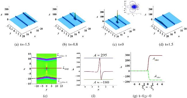
Figure 7. (a)–(d): The evolution of an asymmetric rogue-lump on the background of two bright solitons with parameters α = 1, β = 1, γ = −1, p = 1, $\overline{{\xi }_{1}}=2\pi ,\overline{{\xi }_{2}}=-2\pi ,{b}_{1}=10,{b}_{2}=0$. (e): The trajectories of two solitons and the asymmetric rogue-lump wave in panel (c). (f): The evolution of the asymmetric rogue-lump wave at y = 0 in panel (c). (g): The evolution of the amplitude ( |
The evolutions of ${A}_{{\rm{Max}}}$ and A${}_{{\rm{Min}}}$ are shown in figure 7(g), and the rogue-lump wave only appears as $\overline{{\xi }_{1}}+\overline{{\xi }_{2}}\gg 1$, which matches figures 7(a)–(d). The maximum and minimum values approach to the background plane, which means that this rogue-lump disappears. In this case, we analyze the dynamic behavior of two solitons, and the distance between the two solitons is as follows
$\begin{eqnarray}\begin{array}{l}{L}_{{\rm{s}}{\rm{o}}{\rm{l}}{\rm{i}}{\rm{t}}{\rm{o}}{\rm{n}}}^{(2)}-{L}_{{\rm{s}}{\rm{o}}{\rm{l}}{\rm{i}}{\rm{t}}{\rm{o}}{\rm{n}}}^{(1)}=2\mathrm{ln}\left[2{{\rm{e}}}^{2(\overline{{\xi }_{2}}-\overline{{\xi }_{1}})}\right.\\ \left.\,+\,2{\left(12{\rm{t}}-x+\frac{1}{2}\right)}^{2}+24{y}^{2}+\frac{1}{2}\right]-2(\overline{{\xi }_{2}}-\overline{{\xi }_{1}})\\ \,\gt \,2\mathrm{ln}\left[2{{\rm{e}}}^{2(\overline{{\xi }_{2}}-\overline{{\xi }_{1}})}\right]-2(\overline{{\xi }_{2}}-\overline{{\xi }_{1}})\gt 0.\end{array}\end{eqnarray}$
Clearly, the distance between two solitons is always greater than zero, indicating that these two solitons are always separated from each other, as shown in figure 8.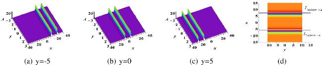
Figure 8. The time evolution of the semi-rational solution ( |
Taking in equation (35 ) $\alpha =1,\beta =1,\gamma =-1,p=1,\overline{{\xi }_{1}}=2\pi ,\overline{{\xi }_{2}}=-2\pi ,{b}_{1}=0,{b}_{2}=0$, the semi-rational solution (35 ) describes the evolution of a symmetrical rogue-lump wave on two soliton planes, see figure 9. The expression for the rogue-lump wave is as follows
$\begin{eqnarray}{A}_{{\rm{r}}{\rm{o}}{\rm{g}}{\rm{u}}{\rm{e}}-{\rm{l}}{\rm{u}}{\rm{m}}{\rm{p}}}=\frac{24\,{(24t-2x+1)}^{2}+1152{y}^{2}+24}{{\left[2\,{\left(12t-x+\frac{1}{2}\right)}^{2}+24{y}^{2}+\frac{1}{2}\right]}^{2}}.\end{eqnarray}$
This rogue-lump wave has the following three extreme points $\begin{eqnarray}\begin{array}{l}{l}_{1}(x,y)=(12t+\frac{1}{2},\,\,0),\\ {l}_{2}(x,y)=(12t+\frac{1}{2}+\frac{\sqrt{3}}{2},\,\,0),\\ {l}_{3}(x,y)=(12t+\frac{1}{2}-\frac{\sqrt{3}}{2},\,\,0).\end{array}\end{eqnarray}$
The maximum amplitude is obtained at l1(x, y), and the maximum amplitude is $\begin{eqnarray}\begin{array}{l}{A}_{{\rm{Max}}}=A{| }_{{l}_{1}}\\ =\,96\frac{\left\{\begin{array}{cc} & 48{{\rm{e}}}^{(16t+4\pi +1)}+3{{\rm{e}}}^{(48t+4\pi +3)}+4{{\rm{e}}}^{(32t+8\pi +2)}\\ & +48{{\rm{e}}}^{(32t+2)}+64{{\rm{e}}}^{(16t-4\pi +1)}+4{{\rm{e}}}^{(48t-4\pi +3)}\end{array}\right\}}{{\left[2{{\rm{e}}}^{(16t+4\pi +1)}+{{\rm{e}}}^{(32t+2)}+8{{\rm{e}}}^{(16t-4\pi +1)}+16\right]}^{2}}.\end{array}\end{eqnarray}$
The lump wave reaches the minimum amplitude at l2(x, y) and l3(x, y), and the minimum amplitude is $\begin{eqnarray}{A}_{{\rm{Min}}-1}=A{| }_{{l}_{2}}=\frac{\left\{\begin{array}{cc} & (576-384\sqrt{3}){{\rm{e}}}^{(48t+4\pi +3+3\sqrt{3})}-768{{\rm{e}}}^{(32t+8\pi +2+2\sqrt{3})}+384{{\rm{e}}}^{(48t-4\pi +3+3\sqrt{3})}\\ & +(9216+6144\sqrt{3}){{\rm{e}}}^{(16t+4\pi +1+\sqrt{3})}+4608{{\rm{e}}}^{(32t+2+2\sqrt{3})}+6144{{\rm{e}}}^{(16t-4\pi +1+\sqrt{3})}\end{array}\right\}}{{\left[8{{\rm{e}}}^{(16t+4\pi +1+\sqrt{3})}+{{\rm{e}}}^{(32t+2+2\sqrt{3})}+8{{\rm{e}}}^{(16t-4\pi +1+\sqrt{3})}+16\right]}^{2}},\end{eqnarray}$
$\begin{eqnarray*}\begin{array}{l}{A}_{{\rm{Min}}-2}=A{| }_{{l}_{3}}=\frac{\left\{\begin{array}{cc} & (576+384\sqrt{3}){{\rm{e}}}^{(48t+4\pi +3-3\sqrt{3})}-768{{\rm{e}}}^{(32t+8\pi +2-2\sqrt{3})}+384{{\rm{e}}}^{(48t-4\pi +3-3\sqrt{3})}\\ & +(9216-6144\sqrt{3}){{\rm{e}}}^{(16t+4\pi +1+\sqrt{3})}+4608{{\rm{e}}}^{(32t+2-2\sqrt{3})}+6144{{\rm{e}}}^{(16t-4\pi +1-\sqrt{3})}\end{array}\right\}}{{\left[8{{\rm{e}}}^{(16t+4\pi +1+\sqrt{3})}+{{\rm{e}}}^{(32t+2+2\sqrt{3})}+8{{\rm{e}}}^{(16t-4\pi +1+\sqrt{3})}+16\right]}^{2}},\end{array}\end{eqnarray*}$
where ${A}_{{\rm{Max}}}\to 96$ and AMin → −12, as seen in figure 9(d). Obviously, the evolution of the maximum and minimum amplitudes of rogue-lump wave in panel (e) perfectly matches the evolution of the three-dimensional plots in panels (a)–(c).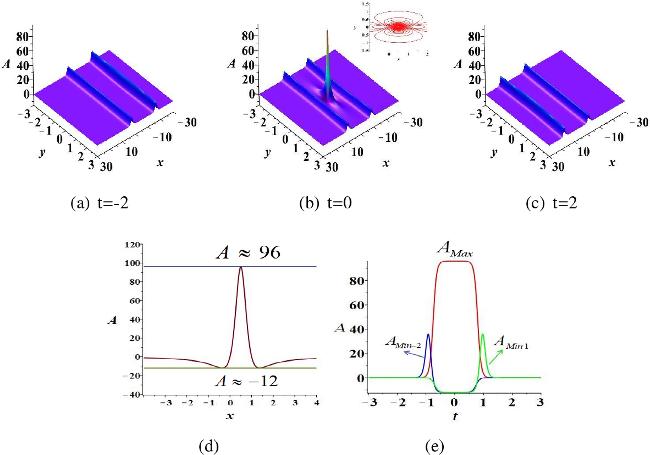
Figure 9. (a)–(c): The evolution of a symmetric rogue-lump on the background of two bright solitons with parameters α = 1, β = 1, γ = −1, $p=1,\overline{{\xi }_{1}}=-2\pi ,\overline{{\xi }_{2}}=2\pi $, b1 = 0, b2 = 0. (d): The evolution of symmetric rogue-lump wave at y = 0 in panel (c). (e): The evolution of the amplitude of symmetric rogue-lump wave. |
3.2. High-order doubly localized two-dimensional rogue waves
In what follows, the full resonant collision of high-order semi-rational solutions are derived. The high-order semi-rational solutions (32 ) of the nonlocal KP equation (5 ) in theorem 2 demonstrate that M rogue-lump waves appear from (M + 1) solitons and then disappear from these solitons for M > 1. Then, we investigate the dynamics of these high-order semi-rational solutions (32 ). The case of N = 2 is first considered. In this case, the following second-order semi-rational solutions are obtained 48 ) can be divided into four categories.
$\begin{eqnarray}\begin{array}{l}A=\left(\frac{12\beta }{\alpha }{\partial }_{xx}+{b}_{1}{\partial }_{xxt}+{b}_{2}{\partial }_{xxy}\right)\,\,(\mathrm{ln}f),\\ B=\left(\frac{12\beta }{\alpha }{\partial }_{xx}-{b}_{1}{\partial }_{xxt}-{b}_{2}{\partial }_{xxy}\right)\,\,(\mathrm{ln}f),\end{array}\end{eqnarray}$
with $\begin{eqnarray}f(x,y,t)=\left|\begin{array}{ccc}{m}_{11}^{(0)} & {m}_{12}^{(0)} & {m}_{13}^{(0)}\\ {m}_{21}^{(0)} & {m}_{22}^{(0)} & {m}_{23}^{(0)}\\ {m}_{31}^{(0)} & {m}_{32}^{(0)} & {m}_{33}^{(0)}\end{array}\right|,\end{eqnarray}$
here, ${m}_{{\rm{i}},j}^{(n)}$ are shown in theorem 2. For convenience, taking α = 1, β = 1, γ = − 1, ai0 = 1, aij = 0 (i, j = 1, 2, 3), these solutions contain four free complex parameters $\overline{{\xi }_{1}},\overline{{\xi }_{2}},\overline{{\xi }_{3}}$, and p. The dynamic behaviors of this second-order solution (The corresponding semi-rational solutions (48 ) describe the dynamic evolution of two rogue-lump waves that appear synchronously and disappear asynchronously on three bright soliton background planes when $\overline{{\xi }_{1}}\gg 0,\overline{{\xi }_{1}}\gg \overline{{\xi }_{3}}\gg \overline{{\xi }_{2}},\overline{{\xi }_{2}}\ll 0$. As shown in figure 10, the corresponding solution describes a three solitons background plane in the initial state, then two lumps suddenly appear from the leftmost soliton. In the middle state, these two lumps pass through the middle soliton, leaving only one lump wave. Finally, the remaining lump wave quickly disappears into the rightmost soliton, and only three solitons remain on the plane.
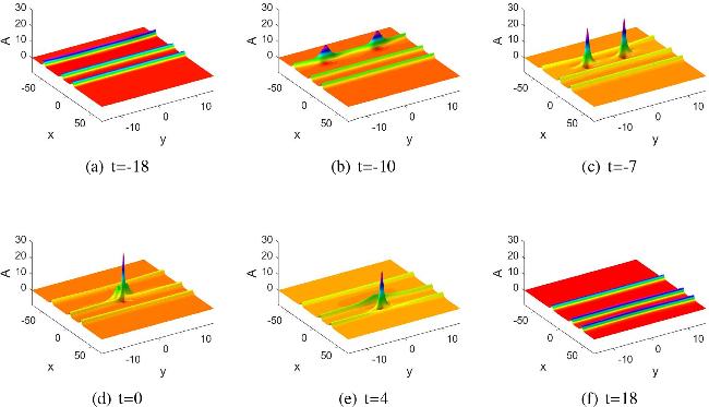
Figure 10. The evolution of semi-rational solutions ( |
The corresponding semi-rational solutions (48 ) demonstrate the dynamic evolution of two rogue-lump waves that appear and disappear synchronously on three bright soliton background planes when $\overline{{\xi }_{1}}\gg 0,\overline{{\xi }_{1}}\gg \overline{{\xi }_{2}}\gg \overline{{\xi }_{3}},\overline{{\xi }_{3}}\ll 0$. As depicted in figure 11, in the initial stage, the semi-rational solution shows a three solitons background plane, then two lumps suddenly appear from the leftmost soliton. In the middle stage, these two lumps go straight through to the middle soliton. Finally, the two lumps quickly disappears into the rightmost soliton.
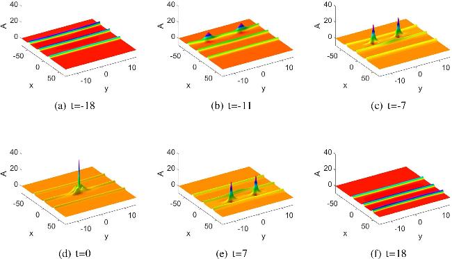
Figure 11. The evolution of semi-rational solutions ( |
The corresponding semi-rational solutions (48 ) characterize the dynamic evolution of two rogue-lump waves that appear asynchronously and disappear synchronously on three bright soliton background planes, when $\overline{{\xi }_{2}}\gg 0,\overline{{\xi }_{2}}\gg \overline{{\xi }_{1}}\gg \overline{{\xi }_{3}},\overline{{\xi }_{3}}\ll 0$. As seen in figure 12, the semi-rational solution shows a three solitons background plane at the initial moment, then one lumps suddenly appear from the leftmost soliton. In the intermediate state, this lump passes through the middle soliton, while another lump is generated from the middle soliton. Finally, the two lumps quickly disappears into the rightmost soliton.
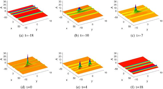
Figure 12. The evolution of semi-rational solutions ( |
The corresponding semi-rational solutions (48 ) characterize the dynamic evolution of three solitons and does not involve rogue-lump wave, when $\overline{{\xi }_{3}}\gg 0,\overline{{\xi }_{3}}\gg \overline{{\xi }_{2}}\gg \overline{{\xi }_{1}},\overline{{\xi }_{1}}\ll 0$. As seen in figure 13, the background plane always consists of three bright solitons, which are different from the three types of dynamical behaviors of the above corresponding solutions.
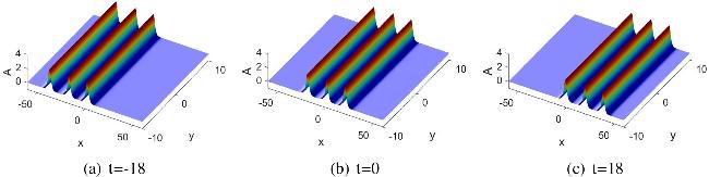


Figure 13. The evolution of semi-rational solutions ( |
4. Conclusions
The rogue waves, which are localized in space and time, are a frontier research area in nonlinear science and applied physics. The known doubly localized rogue waves that have standard symmetric shapes only occur in local and nonlocal one-dimensional nonlinear systems. However, the ocean rogue waves and the rogue waves in two-dimensional media have asymmetric shapes. Therefore, the investigation of asymmetric rogue wave solutions in high-dimensional real nonlocal integrable systems is of practical significance and a novel work.
In this paper, a nonlocal KP equation is discussed using the Hirota bilinear method and the KP hierarchy reduction method. We have derived the semi-rational solutions of the partial resonant collision and full resonant collision formed by lumps and solitons. Due to the semi-localization in time of the lump waves during the interaction between lumps and solitons, this phenomenon is called partial resonant collision. The lump waves in partial resonant collisions are also known as partial rogue waves. The lumps are localized in space variables x, y and time variable t during the interaction between lumps and solitons, and these lump waves are called doubly localized rogue waves, which are generated by the full resonant collision. In this paper, the waveform of the lump is completely symmetrical when b1b2 = 0, otherwise it is not.
In the case of partial resonant collisions between lumps and solitons, the semi-rational solutions given by theorem 1, generated by the partial resonant collision of lump waves and solitons, reduce to the lump waves as αsj = 0. We have obtained the semi-rational solution formed by the resonant collision of one lump and one soliton taking N = 1, ni = 1 in theorem 1, where the lump wave is generated from the soliton and propagates forward at a constant velocity and amplitude. Taking N = 1, ni≥2 in theorem 1, the semi-rational solutions generated by the resonant collision of multiple lump waves and one soliton are given. These lump waves move along a certain curve and eventually converge on a straight line under appropriate values of the parameters. Taking N ≥ 2, ni = 1 in theorem 1, the resonant collision solutions of the interaction between multiple lumps and multiple solitons are proposed, in which the lump wave undergoes two successive fusions. Clearly, the lump waves appear at the initial time (i.e., t → −∞) in the evolution process of these semi-rational solutions.
In case of full resonant collisions between lumps and solitons, the simplest full resonant collision of the interaction between one lump and two solitons is first derived taking M = 1 in theorem 2. The dynamics of this semi-rational solution include two cases, one of which is the appearance of a lump wave from a soliton and its annihilation into another soliton. Another scenario is that this semi-rational solution describes two separate bright solitons. For larger M, the semi-rational solutions of the nonlocal KP equation in theorem 2 demonstrate that M rogue-lump waves appear from (M + 1) solitons and then disappear from these solitons. These lump waves are localized in both time variable t and space variables (x, y), and are known as doubly localized rogue waves.
The results reported in this paper reveal new wave structures in high-dimensional real nonlocal systems, providing a reference for future related research. The next natural extension of this work is the study of the partial and full resonant collision behaviors between lump waves and breather waves.