

1. Introduction
Computational analysis of partial differential equations (PDEs) has traditionally relied on high-resolution spatial discretization. While effective, this approach becomes prohibitively expensive for capturing long-term dynamical behavior. A key simplifying feature for a broad class of dissipative evolution equations is that their asymptotic dynamics are inherently low-dimensional [1–5]. This property is rigorously formalized in the theory of inertial manifolds [5–9]. An inertial manifold is a finite-dimensional, positively invariant Lipschitz manifold that exponentially attracts all solution trajectories and contains the global attractor. The flow restricted to this manifold is described by a finite system of ordinary differential equations, known as the inertial form.
Although the existence of inertial manifolds has been established for canonical systems such as the Cahn–Hilliard [10], Ginzburg–Landau [11], and Kuramoto–Sivashinsky (KS) equations [12–16], their explicit construction remains a great challenge. In practice, one may resort to approximate inertial manifolds, which aim to capture the long-time dynamics with a drastically reduced set of variables. The development of effective approximation methods extends across various classes of dynamical systems, from integrable solutions for ordinary differential equations [17, 18] to analytical studies of coherent structures and bifurcations in fractional PDEs [19, 20]. However, these techniques are usually good for specific types of solutions and hard to apply globally for all the solutions on the manifold.
A common paradigm in approximate inertial manifold construction is to distinguish between a small set of resolved (slow) modes and a large set of unresolved (fast) modes that are assumed to be enslaved to the slow ones. Methods such as nonlinear Galerkin schemes [8, 21–25] assume that the fast modes adjust instantaneously to the slow ones, which replace the fast dynamics with an algebraic expression derived by neglecting their time derivatives. Similarly, pseudo-steady-state closures [7–9, 26–28] set the time derivatives of the fast modes to zero and solve the resulting algebraic system for the fast variables in terms of the slow ones. While these approximations can be effective when time scales are well separated, they may lose validity near bifurcations or in transient regimes where the adiabatic assumption breaks down [25, 26]. Even when the assumption holds, they fix the form of the closure from the beginning, making it difficult to systematically improve the accuracy without changing the underlying ansatz. Because the closure is imposed rather than derived from a consistent expansion, there is also no built-in way to estimate the error introduced or to proceed to higher-order corrections in a controlled manner. What is missing is a first-principle, order-by-order constructive procedure that derives the slaving relation directly from the equations, instead of imposing it, and provides a systematic route to refinement with explicit control over the neglected terms. The renormalization group (RG) method offers precisely such a framework.
The RG method provides a natural candidate for such a procedure. It was first proposed in theoretical physics for removing singularities in the perturbation theory of quantum physics [29], and later developed by Wilson and others into a powerful tool for studying scale invariance and critical phenomena in statistical physics [30–32]. The idea was extended to the asymptotic analysis of differential equations by Chen, Goldenfeld, and Oono [33, 34] as a perturbative tool for deriving long-time approximate solutions. In this formulation, RG systematically eliminates secular terms in asymptotic expansions to obtain an amplitude equation describing the slow envelope dynamics. This differs in technical details from Wilson-type RG commonly used in statistical physics, which integrates out spatial scales to find critical exponents. Despite these differences in implementation, both approaches share the same conceptual core: the systematic elimination of irrelevant scales or degrees of freedom (DOF) to obtain an effective description of the long-wavelength or long-time behavior. Kunihiro [35–37] later gave the method a geometric interpretation, showing that the RG solution forms an envelope of naive perturbation expansions and thereby implicitly organizes dynamics along invariant structures. This geometric viewpoint was further formalized by Ziane [38] and DeVille et al [39], who used averaging operators to establish rigorous error estimates and connect RG asymptotics with the stability of invariant manifolds. Building directly on this foundation, Chiba [40–42] developed the restricted RG method, which explicitly links RG reduction to center manifold theory for finite-dimensional systems. By restricting the RG equation to the center subspace, Chiba demonstrated that the method systematically constructs both an approximate center manifold and the reduced flow on it. A key theoretical result is the structural correspondence: if the reduced RG equation admits a normally hyperbolic invariant manifold, then the original system possesses a diffeomorphic copy, thereby embedding RG reduction firmly within invariant manifold theory [41]. More recently, Chiba [43] has further extended the RG framework to provide a novel constructive method for deriving normal forms of smooth vector fields, reinforcing its role as a general geometric tool in dynamical systems. However, while this body of work provides a rigorous foundation for finite-dimensional systems, its extension to infinite-dimensional dissipative PDEs presents distinct challenges. In such systems, the asymptotic dynamics are governed by an inertial manifold. The key difficulties include handling a continuous spectrum of linear modes, selecting a finite set of resolved variables from infinitely many candidates, and controlling the convergence of perturbative expansions in infinite dimensions.
We bridge this gap by adapting the RG framework to the construction of approximate inertial manifolds for dissipative PDEs. We work systematically in a spectral space and introduce a clear criterion for selecting dynamically relevant modes: linearly unstable and weakly damped modes are retained, while the effects of strongly damped modes are eliminated through the renormalization process. This procedure naturally resolves the arbitrary constants of perturbation theory, yielding a uniformly valid reduced model and providing a principled way to identify the active DOF. We demonstrate this framework by constructing an approximate inertial manifold for the KS equation [44, 45], a canonical dissipative PDE known for its low-dimensional asymptotic dynamics and rich spatiotemporal chaos. A defining feature of the method is that it simultaneously determines the geometry of the manifold—expressed through explicit algebraic relations that enslave higher Fourier modes to the dominant ones—and the autonomous flow on it. Notably, the approach does not assume the form of the manifold in advance. Instead, the manifold and its dynamics emerge self-consistently from the renormalization process, which inherently captures the nonlinear feedback from fast, strongly damped modes onto the slow, active ones. The outcome is a rigorously derived, low-dimensional model that balances computational efficiency with faithful reproduction of the system's dynamical features.
The paper is structured as follows. We first detail the theoretical basis for using the RG method to approximate inertial manifolds and outline the systematic reduction procedure. We then apply this framework to the KS equation, providing guidelines for mode selection and truncation. Finally, we validate the approach through comprehensive numerical simulations, assessing its accuracy in reproducing waveform evolution, bifurcation behavior, and statistical properties across a range of parameters. The method establishes a generalizable framework for model reduction of high-dimensional dissipative PDEs.
2. Renormalization group method for approximate inertial manifolds
This section details a systematic application of the RG method to construct low-dimensional approximate inertial manifolds for a class of dissipative PDEs. The approach is built upon the multiscale structure inherent in such systems, where the dynamics naturally separate into a finite set of slow, active modes and a complement of fast, strongly damped ones. The RG procedure does not presuppose the manifold's form; instead, it self-consistently derives both the geometry of the approximate inertial manifold and the reduced dynamical system on it through a controlled perturbation expansion. This yields an autonomous set of equations for the slow modes alone, effectively closing the dynamics without relying on ad-hoc truncations.
The method is particularly well-suited for PDEs that possess a spectral gap or clear time-scale separation—a property shared by many dissipative evolution equations that admit an inertial manifold. To demonstrate and validate the framework concretely, we focus on the KS equation, a prototypical model of spatiotemporal chaos and weak turbulence. The KS equation is an ideal testbed for several reasons: it exhibits a well-documented separation between unstable/low-damped modes and strongly stable ones, and substantial numerical evidence suggests its long-term dynamics reside on a finite-dimensional inertial manifold over a wide parameter range [27, 46]. Moreover, it retains key structural features—such as quadratic nonlinearity, dissipative regularization, and fundamental symmetries—that are central to more complex fluid systems like the Navier–Stokes equation [47–49]. Thus, while the analysis is carried out explicitly for the KS equation, the underlying procedure is general in nature and can be adapted to other dissipative PDEs with similar scale-separated dynamics.
We begin with the one-dimensional KS equation with periodic boundary conditions:
$\begin{eqnarray}{u}_{t}=\epsilon {({u}^{2})}_{x}-{u}_{xx}-\nu {u}_{xxxx},\quad u(t,x)=u(t,x+2\pi ),\end{eqnarray}$
where ν > 0 is a dissipation parameter. The strong fourth-order dissipation creates a spectral gap, which confines the long-term dynamics to a finite set of large-scale Fourier modes. The 'small parameter' ε is introduced here as a formal bookkeeping device to track the order of nonlinearity in the subsequent perturbation expansion. Following the standard RG approach, it is set to ε = 1 at the end of the calculation, which corresponds to resumming the original nonlinearity.To obtain a finite-dimensional representation, we expand the solution as a power series in ε:
$\begin{eqnarray}\begin{array}{rcl}u(t,x) & = & {u}_{0}(t,x)+\epsilon {u}_{1}(t,x)+{\epsilon }^{2}{u}_{2}(t,x)\\ & & +{\epsilon }^{3}{u}_{3}(t,x)+\cdots \,.\end{array}\end{eqnarray}$
Substituting this expansion into equation (1 ) and grouping terms by powers of ε gives a sequence of linear equations:
$\begin{eqnarray}\begin{array}{l}{ \mathcal O }({\epsilon }^{0}):\quad {\partial }_{t}{u}_{0}={ \mathcal L }{u}_{0},\\ { \mathcal O }({\epsilon }^{1}):\quad {\partial }_{t}{u}_{1}={ \mathcal L }{u}_{1}+{{ \mathcal N }}_{1}({u}_{0}),\\ { \mathcal O }({\epsilon }^{2}):\quad {\partial }_{t}{u}_{2}={ \mathcal L }{u}_{2}+{{ \mathcal N }}_{2}({u}_{0},{u}_{1}),\\ { \mathcal O }({\epsilon }^{3}):\quad {\partial }_{t}{u}_{3}={ \mathcal L }{u}_{3}+{{ \mathcal N }}_{3}({u}_{0},{u}_{1},{u}_{2}),\end{array}\end{eqnarray}$
where ${ \mathcal L }=-\nu {\partial }_{x}^{4}-{\partial }_{x}^{2}$ is the linear operator. The nonlinear terms are $\begin{eqnarray}\begin{array}{l}{{ \mathcal N }}_{1}({u}_{0})=2{u}_{0}\frac{\partial {u}_{0}}{\partial x},\\ {{ \mathcal N }}_{2}({u}_{0},{u}_{1})=2{u}_{0}\frac{\partial {u}_{1}}{\partial x}+2{u}_{1}\frac{\partial {u}_{0}}{\partial x},\\ {{ \mathcal N }}_{3}({u}_{0},{u}_{1},{u}_{2})=2{u}_{2}\frac{\partial {u}_{0}}{\partial x}+2{u}_{1}\frac{\partial {u}_{1}}{\partial x}+2{u}_{0}\frac{\partial {u}_{2}}{\partial x}.\end{array}\end{eqnarray}$
We now construct the solution order by order. The leading-order solution consists of the Fourier modes that are either linearly unstable or weakly damped. These modes correspond to the eigenfunctions of ${ \mathcal L }$ and form a natural basis from which an approximate inertial manifold can be constructed:
$\begin{eqnarray}{u}_{0}(t,{t}_{0},x)=\displaystyle \sum _{k=-N}^{N}{a}_{k}({t}_{0})\,{{\rm{e}}}^{{\lambda }_{k}(t-{t}_{0})+{\rm{i}}kx},\end{eqnarray}$
where λk = k2 − νk4 is the linear growth rate and ak are complex amplitudes. For real-valued solutions, the symmetry condition ${a}_{-k}=\overline{{a}_{k}}$ holds, which halves the number of independent real variables and simplifies the reduced system. The integer N is chosen so that all modes with ∣k∣ > N are strongly damped (λk < 0), ensuring that the essential dynamics is captured by this set of N modes. We emphasize that while such symmetry further streamlines the construction, the RG procedure itself does not rely on it and remains applicable to systems without symmetry. Similarly, although a clear spectral gap facilitates mode selection, the method does not strictly require it—strongly damped modes are systematically eliminated through perturbation, and weakly damped modes can be retained even when the gap is not so distinct.To obtain an expansion that remains valid over long times, we use the RG method. In this approach, the amplitudes ak are allowed to depend on the initial time t0 in such a way that the perturbative series stays valid as t0 changes. The goal is to derive evolution equations for ak(t0) that describe the dynamics on a low-dimensional manifold.
At higher orders, nonlinear interactions generate forcing terms of the form
$\begin{eqnarray*}{{\rm{e}}}^{m(t-{t}_{0})+{\rm{i}}nx},\quad \,\rm{where}\,m={\lambda }_{{k}_{1}}+{\lambda }_{{k}_{2}},\quad n={k}_{1}+{k}_{2},\end{eqnarray*}$
with k1, k2 in the set {−N, …, N}. If the resulting wavenumber n satisfies ∣n∣ ≤ N, the spatial pattern einx matches one of the basis modes. Including such a term directly would create an independent time evolution for the same spatial mode, breaking the unique parameterization of the manifold. To avoid this problem, we modify the particular solution for these overlapping cases as $\begin{eqnarray*}{{\rm{e}}}^{m(t-{t}_{0})+{\rm{i}}nx}-{{\rm{e}}}^{{\lambda }_{n}(t-{t}_{0})+{\rm{i}}nx}.\end{eqnarray*}$
This subtraction is zero at t = t0, so it does not change the definition of the leading amplitude an(t0). It also ensures that the possibly existing small divisors before this exponential term are canceled out in the resulting RG equation.If m ≈ λn for a mode with ∣n∣ > N (a near-resonance with a strongly damped mode), the denominator m − λn becomes small and may produce anomalously large coefficients. Should this occur, it would signal that the corresponding mode should be included in the resolved set N. In the parameter regimes studied here, however, numerical evaluation confirms that such near-resonances do not arise, and the expansion remains well behaved.
As a result, the pth order correction takes the form
$\begin{eqnarray}\begin{array}{rcl}{u}_{p}(t,x) & = & \displaystyle \sum _{| n| \leqslant N}{c}_{p}^{(m,n)}\left({{\rm{e}}}^{m(t-{t}_{0})+{\rm{i}}nx}-{{\rm{e}}}^{{\lambda }_{n}(t-{t}_{0})+{\rm{i}}nx}\right)\\ & & +\displaystyle \sum _{| n| \gt N}{c}_{p}^{(m,n)}\,{{\rm{e}}}^{m(t-{t}_{0})+{\rm{i}}nx},\end{array}\end{eqnarray}$
where each coefficient ${c}_{p}^{(m,n)}$ is a homogeneous polynomial of degree p in the leading amplitudes {a−N, …, aN}. These coefficients are determined algebraically by matching terms in the expansion equations at order ${ \mathcal O }({\epsilon }^{p})$.To extract the evolution of the slow-mode amplitudes, we consider the complete perturbative solution
$\begin{eqnarray}\tilde{u}(t,x):= {u}_{0}(t,x)+\displaystyle \sum _{p\geqslant 1}{\epsilon }^{p}{u}_{p}(t,x).\end{eqnarray}$
We then define the projected amplitude φk(t, t0) as the corresponding Fourier coefficient: $\begin{eqnarray}\begin{array}{rcl}{\phi }_{k}(t,{t}_{0}): & = & \frac{1}{2\pi }{\displaystyle \int }_{0}^{2\pi }\tilde{u}(t,x)\,{{\rm{e}}}^{-{\rm{i}}kx}\,{\rm{d}}x={a}_{k}({t}_{0}){{\rm{e}}}^{{\lambda }_{k}(t-{t}_{0})}\\ & & +\displaystyle \sum _{p\geqslant 1}{\epsilon }^{p}\displaystyle \sum _{m\in {M}_{p}(k)}{c}_{p}^{(m,k)}\left({{\rm{e}}}^{m(t-{t}_{0})}-{{\rm{e}}}^{{\lambda }_{k}(t-{t}_{0})}\right),\end{array}\end{eqnarray}$
where Mp(k) denotes the set of linear combinations $m={\lambda }_{{k}_{1}}+\ldots +{\lambda }_{{k}_{p+1}}$ arising from pth order interactions that affect mode k.The RG condition requires that φk should not depend on the arbitrary choice of initial time t0 when evaluated along the true nonlinear solution. This requirement of time-translation invariance is expressed via the condition [33, 34, 50]
$\begin{eqnarray}{\left.\frac{\partial {\phi }_{k}(t,{t}_{0})}{\partial {t}_{0}}\right|}_{t={t}_{0}}=0,\qquad | k| \leqslant N.\end{eqnarray}$
Differentiating equation (8 ) with respect to t0, evaluating the result at t = t0, and finally setting the formal expansion parameter ε = 1, we obtain the closed system of amplitude equations:
$\begin{eqnarray}\begin{array}{rcl}{\left.\frac{{\rm{d}}{a}_{k}}{{\rm{d}}{t}_{0}}\right|}_{t={t}_{0}} & = & {\lambda }_{k}{a}_{k}({t}_{0})+\displaystyle \sum _{p\geqslant 1}\displaystyle \sum _{m\in {M}_{p}(k)}{c}_{p}^{(m,k)}\left(m-{\lambda }_{k}\right)\\ & = & {F}_{k}\left({\{{a}_{j}({t}_{0})\}}_{| j| \leqslant N}\right),\qquad | k| \leqslant N,\end{array}\end{eqnarray}$
where each Fk is an explicit polynomial determined by the nonlinear couplings. Renaming t0 as t gives the autonomous reduced system governing the slow-mode dynamics on the approximate inertial manifold.The dimension reduction is completed by evaluating the full perturbative solution equation (7 ) at the initial time t = t0: 10 ). Together, equations (10 ) and (12 ) form a reduced model on the approximate inertial manifold.
$\begin{eqnarray}\tilde{u}({t}_{0},x)=\displaystyle \sum _{| k| \leqslant N}{a}_{k}({t}_{0}){{\rm{e}}}^{{\rm{i}}kx}+\displaystyle \sum _{p\geqslant 1}\displaystyle \sum _{| k| \gt N}{c}_{p}^{(m,k)}{{\rm{e}}}^{{\rm{i}}kx},\end{eqnarray}$
which provides the slaving relations: all high-wavenumber amplitudes (∣k∣ > N) are expressed as polynomials of the leading amplitudes. Therefore, the full solution can be reconstructed at any time and position as $\begin{eqnarray}u(t,x)\approx \tilde{u}\left(t,x;{\{{a}_{k}(t)\}}_{| k| \leqslant N}\right),\end{eqnarray}$
with the leading amplitudes evolving according to equation (The construction starts from an observation of the system's inherent scale separation [1, 6]. This is a concrete spectral property, shown in figure 1(a): the linear growth rate λk separates a small set of slowly evolving low-wavenumber modes from a continuum of rapidly damped high-wavenumber ones. The RG expansion uses this fact directly, which designates the slow-mode amplitudes ak(t) as coordinates on the manifold, and then solves the perturbation equations to determine how each fast mode is functionally slaved to these coordinates. The result is an explicit mapping that defines the manifold's local geometry. Figure 1(b) gives a tangible example of one such slaving relation, where a higher-mode amplitude depends polynomially on two leading slow amplitudes. This surface itself is a piece of the approximate inertial manifold.
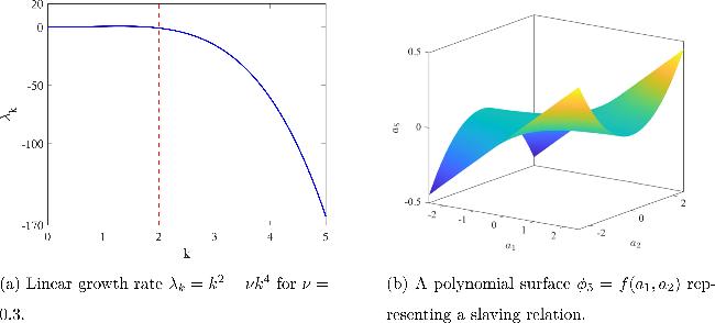
Figure 1. Visualizing the RG construction of an approximate inertial manifold. (a) The linear spectrum exhibits the different dissipation rates that defines the slow variables serving as manifold coordinates. (b) A concrete slaving relation, derived from the RG expansion, geometrically represents a local piece of the manifold surface. |
However, a direct perturbation solution would contain inconsistent terms that grow without bound in time, breaking the expansion's long-time validity. The key step of the RG method is to impose a consistency condition that removes these terms [33, 34]. This is achieved through renormalization, by allowing the initially constant amplitudes ak(t0) to evolve in time. The requirement of a uniformly valid expansion then uniquely determines their evolution, yielding the closed set of RG equations equation (10 ). In this way, the RG method simultaneously constructs both the approximate inertial manifold and the reduced dynamics on it. It determines the manifold by finding the slaving relations of fast modes to slow ones, as shown geometrically in figure 1(b), and retrieves the dynamics by computing the RG equations for the slow-mode evolution. Both are obtained directly from the original equations without any prior assumption about the manifold's shape.
The accuracy and computational efficiency of the resulting low-dimensional model are governed by two principal choices: the selection of retained Fourier modes and the truncation order of the expansion. A minimal guideline for mode selection is to include all linearly unstable modes—for the KS equation, those wavenumbers k satisfying λk = k2 − νk4 > 0, as visualized in figure 1(a). To capture nonlinear saturation and more complex phenomena such as chaos, it is often necessary to also incorporate a few of the most weakly damped stable modes. This selection can be informed by numerical diagnostics, such as Lyapunov exponent spectra or attractor dimension estimates [4, 51], and refined through targeted experimentation.
The choice of truncation order represents a balance between accuracy and algebraic complexity. For polynomial nonlinearities like those in the KS equation, the dominant energy transfer and saturation mechanisms are typically captured by the lowest-order nonlinear couplings—quadratic and cubic terms [52]. In practice, truncating the expansion at third or fourth order is sufficient to produce a globally accurate approximation across a wide parameter range. Theoretically, carrying the expansion to infinite order would recover the exact inertial manifold, but the algebraic complexity grows rapidly beyond the first few orders. In actual computations, one must weigh whether to include higher-order terms or to retain more Fourier modes in the leading set, as both choices increase the dimension and algebraic burden of the reduced model. Thus, the appropriate truncation is ultimately determined through numerical validation, ensuring that the reduced model reproduces key dynamical features—steady states, periodic orbits, and chaotic attractors—while retaining manageable complexity.
3. Applications
We evaluate the performance of the RG method through a systematic validation strategy that progresses from basic accuracy checks to more demanding structural assessments. The initial focus is on waveform fidelity, examining how closely the reduced model reproduces instantaneous spatial patterns compared to full direct numerical simulations (DNS). While matching these patterns provides a necessary baseline, it does not guarantee that the model captures the underlying dynamical organization. A deeper level of validation therefore considers bifurcation behavior, testing whether the reduced model reproduces the qualitative transitions between steady states, periodic oscillations, and chaotic dynamics at the appropriate parameter values. Beyond this, we assess parametric robustness by applying the method across a range of dissipation values ν, ensuring it remains effective as the system's mathematical characteristics vary.
All comparisons are made against reference solutions from high-resolution DNS. The simulations employ a Fourier–Galerkin discretization with a sufficient number of modes to resolve all dynamically relevant scales. Time integration employs a fourth-order Runge–Kutta scheme with Δt = 10−3. To maintain computational tractability while preserving rich dynamics, we restrict the analysis to symmetric solutions: odd symmetry u(x, t) = −u(−x, t) in one dimension and even symmetry u(t, x, y) = u(t, −x, −y) in two dimensions.
The following sections apply this validation framework to both one-dimensional and two-dimensional configurations of the KS equation. We first present results for the one-dimensional case, where the RG method achieves substantial dimensionality reduction while maintaining dynamical accuracy. We then extend the analysis to two dimensions, examining how the method scales to handle increased spatial complexity. Throughout this evaluation, we document both the degree of reduction achieved and the fidelity preserved across different dynamical regimes.
3.1. One-dimensional Kuramoto–Sivashinsky equation
Following the computational setup described above, the reference DNS for the 1D case uses 31 Fourier modes (62-dimensional state space) [51]. In contrast, the RG method achieves a substantial reduction to only 2–12 real DOF within the odd-symmetry subspace.
Basis modes are selected based on linear stability: for each ν, we retain all linearly unstable modes ($| k| \lt 1/\sqrt{\nu }$) along with additional weakly damped modes needed for accurate nonlinear description. A key parameter in the RG construction is the truncation order of the perturbative expansion. We monitor the magnitude of the coefficients ${c}_{p}^{(m,k)}$ generated at each order p. The expansion is truncated at order p when the coefficients at the next order p + 1 become sufficiently small. To quantify the accuracy of a given truncated model, we define the error indicator η as the maximum absolute value among all coefficients $| {c}_{p+1}^{(m,k)}| $ at the first omitted order. This value serves as a practical, a posteriori estimate of the truncation error inherent in the model. The effectiveness of this truncation, and the trade-off between increasing the nonlinear order versus including more slow modes in the leading set, is quantified in table 1. The table shows how a higher truncation order or a larger set of retained modes leads to a smaller error indicator η, indicating a more accurate approximation.
Table 1. Progression of the RG model accuracy with increasing nonlinear order and number of slow modes. |
| ν | $1/\sqrt{\nu }$ | Number of modes | Max nonlinearity | Achieved η | |
|---|---|---|---|---|---|
| Steady state | 0.3 | 1.83 | 2 | cubic (a3) | 10−3 |
| 0.3 | 1.83 | 2 | quartic (a4) | 10−5 | |
| 0.3 | 1.83 | 4 | cubic (a3) | 10−7 | |
| 0.24 | 2.04 | 2 | cubic (a3) | 10−3 | |
| 0.24 | 2.04 | 2 | quartic (a4) | 10−6 | |
| | |||||
| Periodic | 0.059 | 4.12 | 8 | cubic (a3) | 10−3 |
| 0.059 | 4.12 | 8 | quartic (a4) | 10−7 | |
| 0.059 | 4.12 | 10 | cubic (a3) | 10−6 | |
| 0.0555 | 4.24 | 8 | cubic (a3) | 10−3 | |
| | |||||
| Chaos | 0.029910 | 5.78 | 10 | quartic (a4) | 10−2 |
| 0.029910 | 5.78 | 12 | quartic (a4) | 10−4 | |
| 0.02 | 7.07 | 12 | quartic (a4) | 10−3 | |
| 0.02 | 7.07 | 14 | quartic (a4) | 10−6 | |
Number of modes counts the leading Fourier modes (with $| k| \leqslant {k}_{\max }$) retained in the leading-order solution u0(t, x). Max nonlinearity is the highest polynomial order included in the RG expansion. Error indicator η is max $| {c}_{p+1}^{(m,k)}| $ at the first omitted order (p + 1), estimating the model's truncation error. A smaller η signifies formally higher computation accuracy. |
As a concrete illustration of the method, we consider the KS equation with dissipation parameter ν = 0.3. For this value, only the mode with wavenumber k = 1 is linearly unstable (λ1 = 0.7). The mode k = 2 is already weakly damped (λ2 = −0.8), while higher modes are strongly damped (λ3 = −15.3, λ4 = −60.8). To capture both the linear instability and the essential nonlinear saturation, we retain both the unstable mode and the first weakly damped mode. We therefore set N = 2 and construct the approximate inertial manifold following the RG procedure outlined in the previous section.
We work in the odd-symmetry subspace u(t, x) = −u(t, −x). Combined with the reality condition, this gives ${a}_{-k}=\overline{{a}_{k}}=-{a}_{k}$, which forces the original complex amplitudes ak to be purely imaginary. It is convenient to absorb the imaginary unit into a real parameter. We therefore write the leading-order solution explicitly in terms of real amplitudes a1, a2 ∈ R as
$\begin{eqnarray}\begin{array}{rcl}{u}_{0}(t,{t}_{0},x) & = & {\rm{i}}{a}_{1}{{\rm{e}}}^{{\lambda }_{1}(t-{t}_{0})}({{\rm{e}}}^{{\rm{i}}x}-{{\rm{e}}}^{-{\rm{i}}x})\\ & & +{\rm{i}}{a}_{2}{{\rm{e}}}^{{\lambda }_{2}(t-{t}_{0})}({{\rm{e}}}^{2{\rm{i}}x}-{{\rm{e}}}^{-2{\rm{i}}x}),\end{array}\end{eqnarray}$
where the factors ia1 and ia2 are the purely imaginary amplitudes appearing in the original Fourier expansion.The first-order correction u1 is found by substituting u0 into the nonlinear term and solving the resulting linear equation:
$\begin{eqnarray}\begin{array}{rcl}{u}_{1}(t,{t}_{0},x) & = & {\rm{i}}\left(-\frac{2{a}_{1}{a}_{2}\left({{\rm{e}}}^{({\lambda }_{1}+{\lambda }_{2})(t-{t}_{0})-{\rm{i}}x}-{{\rm{e}}}^{{\lambda }_{1}(t-{t}_{0})-{\rm{i}}x}\right)}{-1+\nu +{\lambda }_{1}+{\lambda }_{2}}\right.\\ & & +\frac{2{a}_{1}{a}_{2}\left({{\rm{e}}}^{({\lambda }_{1}+{\lambda }_{2})(t-{t}_{0})+{\rm{i}}x}-{{\rm{e}}}^{{\lambda }_{1}(t-{t}_{0})+{\rm{i}}x}\right)}{-1+\nu +{\lambda }_{1}+{\lambda }_{2}}\\ & & +\frac{{a}_{1}^{2}\left({{\rm{e}}}^{2{\lambda }_{1}(t-{t}_{0})-2{\rm{i}}x}-{{\rm{e}}}^{{\lambda }_{2}(t-{t}_{0})-2{\rm{i}}x}\right)}{-2+8\nu +{\lambda }_{1}}\\ & & -\frac{{a}_{1}^{2}\left({{\rm{e}}}^{2{\lambda }_{1}(t-{t}_{0})+2{\rm{i}}x}-{{\rm{e}}}^{{\lambda }_{2}(t-{t}_{0})+2{\rm{i}}x}\right)}{-2+8\nu +{\lambda }_{1}}\\ & & +\frac{6{a}_{1}{a}_{2}{{\rm{e}}}^{({\lambda }_{1}+{\lambda }_{2})(t-{t}_{0})-3{\rm{i}}x}}{-9+81\nu +{\lambda }_{1}+{\lambda }_{2}}\\ & & -\frac{6{a}_{1}{a}_{2}{{\rm{e}}}^{({\lambda }_{1}+{\lambda }_{2})(t-{t}_{0})+3{\rm{i}}x}}{-9+81\nu +{\lambda }_{1}+{\lambda }_{2}}\\ & & \left.+\frac{2{a}_{2}^{2}{{\rm{e}}}^{2{\lambda }_{2}(t-{t}_{0})-4{\rm{i}}x}}{-8+128\nu +{\lambda }_{2}}-\frac{2{a}_{2}^{2}{{\rm{e}}}^{2{\lambda }_{2}(t-{t}_{0})+4{\rm{i}}x}}{-8+128\nu +{\lambda }_{2}}\right).\end{array}\,\end{eqnarray}$
Observe that terms whose wavenumber belongs to the leading set (∣n∣ ≤ 2, e.g. e±2ix and e±ix) appear in the subtracted form ${{\rm{e}}}^{m(t-{t}_{0})+{\rm{i}}nx}-{{\rm{e}}}^{{\lambda }_{n}(t-{t}_{0})+{\rm{i}}nx}$.
Proceeding to the next order, the second-order correction u2 is obtained by the same systematic procedure. Its complete expression is lengthy and therefore provided in full in Appendix .
We form the perturbative expansion $\tilde{u}={u}_{0}+\epsilon {u}_{1}+{\epsilon }^{2}{u}_{2}$ and compute the projected amplitudes φk(t, t0) as defined in equation (8 ):
$\begin{eqnarray*}{\phi }_{k}(t,{t}_{0})=\frac{1}{2\pi }{\int }_{0}^{2\pi }\tilde{u}(t,{t}_{0},x)\,{{\rm{e}}}^{-{\rm{i}}kx}\,{\rm{d}}x,\quad k=1,2.\end{eqnarray*}$
Imposing the RG condition $\frac{\partial {\phi }_{k}}{\partial {t}_{0}}{| }_{t={t}_{0}}=0$ eliminates secular terms. Setting ε = 1 and keeping terms up to cubic order yields the reduced system for the real amplitudes a1 and a2:
$\begin{eqnarray}\left\{\begin{array}{l}\frac{{\rm{d}}{a}_{1}}{{\rm{d}}t}=0.7{a}_{1}+2{a}_{1}{a}_{2}-0.789474{a}_{1}{a}_{2}^{2},\quad \\ \frac{{\rm{d}}{a}_{2}}{{\rm{d}}t}=-0.8{a}_{2}-2{a}_{1}^{2}-1.57895{a}_{1}^{2}{a}_{2}-0.27027{a}_{2}^{3}.\quad \end{array}\right.\end{eqnarray}$
Finally, evaluating at t = t0 gives the slaving relations. Using the notation φk ≔ φk(t0, t0), and noting that ${\phi }_{-k}=-\overline{{\phi }_{k}}$ due to odd symmetry, we obtain
$\begin{eqnarray}\begin{array}{rcl}{\phi }_{1} & = & {\rm{i}}{a}_{1},\\ {\phi }_{2} & = & {\rm{i}}{a}_{2},\\ {\phi }_{3} & = & {\rm{i}}(0.0453721{a}_{1}^{3}+0.394737{a}_{1}{a}_{2}-0.0266714{a}_{1}{a}_{2}^{2}),\\ {\phi }_{4} & = & {\rm{i}}(0.0470297{a}_{1}^{2}{a}_{2}-0.0675676{a}_{2}^{2}),\\ {\phi }_{5} & = & {\rm{i}}(0.0286079{a}_{1}{a}_{2}^{2}),\\ {\phi }_{6} & = & {\rm{i}}(0.00231396{a}_{2}^{3}).\end{array}\end{eqnarray}$
The full solution on the approximate inertial manifold is reconstructed as 15 ). The reduced two-dimensional system equation (15 ) together with these algebraic slaving relations form a closed approximate inertial manifold for the KS equation at ν = 0.3.
$\begin{eqnarray*}u(t,x)=\displaystyle \sum _{k=-6}^{6}{\phi }_{k}(t){{\rm{e}}}^{{\rm{i}}kx}=\displaystyle \sum _{k=1}^{6}\left({\phi }_{k}(t){{\rm{e}}}^{{\rm{i}}kx}-{\phi }_{k}(t){{\rm{e}}}^{-{\rm{i}}kx}\right),\end{eqnarray*}$
with φk(t) given above in terms of a1(t) and a2(t), which evolve according to equation (3.1.1. Steady states
The RG model with only 2 real DOF reproduces steady-state solutions across a range of dissipation parameters. Figure 2 compares the spatial profiles from the RG model (red dashed lines) with the DNS reference (blue solid lines) for two representative values: ν = 0.3 and ν = 0.24. Visually, the waveforms are nearly indistinguishable, confirming the model's ability to capture both amplitude and spatial structure.
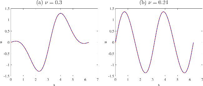
Figure 2. Steady-state solutions of the 1D KS equation. (a) ν = 0.3: a single-hump profile; (b) ν = 0.24: a double-hump profile. Blue solid lines: DNS reference; red dashed lines: 2-degree-of-freedom RG model prediction. |
Quantitatively, table 2 lists the amplitude of the dominant mode (a2) at steady state for the two dissipation values. The magnitude of the DNS amplitude increases from 0.3120 at ν = 0.3 to 0.6748 at ν = 0.24, reflecting the stronger nonlinear saturation required as dissipation weakens. The third-order (cubic) RG model already shows excellent agreement, with relative errors below 0.3%, indicating that a cubic truncation is sufficient for steady-state accuracy. The fourth-order (quartic) RG results coincide exactly with the DNS values, confirming the systematic convergence of the expansion.
Table 2. Dominant mode amplitude a2 at steady state. |
| ν | $\frac{1}{\sqrt{\nu }}$ | DNS | cubic (a3) | quartic (a4) |
|---|---|---|---|---|
| 0.30 | 1.83 | −0.3120 | −0.3118 | −0.3120 |
| 0.24 | 2.04 | −0.6748 | −0.6757 | −0.6748 |
These results validate the robustness of the RG construction, which successfully encodes the balance between linear growth and nonlinear saturation that governs the steady states, and demonstrates a systematic route to high accuracy without ad-hoc tuning.
3.1.2. Periodic dynamics and bifurcation structure
The onset of temporal periodicity in the KS equation occurs via a Hopf bifurcation, which provides a stringent test for reduced-order models. To accurately capture this transition, we use an RG model with sufficiently many modes and a higher-order nonlinear truncation, as guided by the accuracy criteria established earlier.
We visualize the global bifurcation structure using bifurcation diagrams based on the Poincaré map, following the standard procedure [53]. For each value of ν, we integrate the system from random initial conditions until transients decay and record the value of the dominant mode a1 each time the trajectory crosses the Poincaré section defined by ${\dot{a}}_{1}=0$ with ${\dot{a}}_{1}\lt 0$. Sweeping ν across the range of interest yields the characteristic bifurcation tree.
The result is shown in figure 3. The figure compares DNS (black dots) and RG model (red circles) results across two parameter ranges: (a) ν ∈ [0.0585, 0.0605], focusing on the Hopf bifurcation, and (b) ν ∈ [0.055 238, 0.057], covering the first period-doubling cascade and beyond. The characteristic Feigenbaum tree is clearly visible: a single branch of periodic points emerges near ν ≈ 0.059 85, which then splits successively into two, four branches as ν decreases, marking the transition toward chaos. The near-perfect overlap of the black and red markers across the entire parameter range shows that the RG model reproduces this global skeleton with high fidelity. Quantitatively, the Hopf bifurcation point predicted by the RG model differs from the DNS value by less than 0.04%, and the first period-doubling point agrees within 0.18%. This close agreement confirms that the reduced model preserves the essential phase-space organization of the original system.
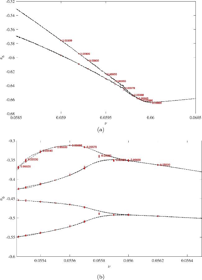
Figure 3. Bifurcation diagrams for the 1D KS equation. (a) ν ∈ [0.0585, 0.0605], showing the Hopf bifurcation; (b) ν ∈ [0.055 238, 0.057], showing the onset of period-doubling. Black dots: DNS; red circles: RG model. |
To examine the local geometry of individual periodic orbits, we compare the performance of RG models with cubic and quartic truncations at a fixed post-bifurcation value ν = 0.059 in figure 4. The upper panels compare the spatial waveforms. In figure 4(a), the cubic model (red dashed line) captures the periodic oscillation but shows a slight overestimation in both peak and trough amplitudes compared to the DNS reference (blue solid line). In contrast, the quartic model in figure 4(b) produces a waveform that is virtually indistinguishable from the DNS profile, with excellent agreement in both amplitude and phase.
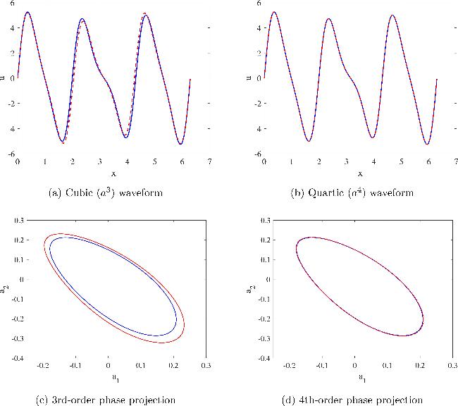
Figure 4. Comparison of RG models with cubic and quartic truncations at ν = 0.059. (a), (b) Spatial waveforms; (c), (d) phase-plane (a1, a2) projections. Blue curves: DNS reference; red curves: RG model. The quartic model shows notably better agreement in phase-space geometry. |
The lower panels display the corresponding phase-plane projections onto the (a1, a2) plane. Both models yield smooth, closed orbits that qualitatively resemble the DNS limit cycle. However, as shown in figure 4(c), the cubic orbit lies slightly outside the DNS reference, reflecting the amplitude overestimation seen in the waveform. Figure 4(d) demonstrates that the quartic orbit overlaps almost perfectly with the DNS trajectory, accurately reproducing the elliptical shape and closure of the true limit cycle.
These visual observations are quantified in table 3. The cubic model already predicts the correct period and orbit geometry, but its mean and maximum amplitudes exceed the DNS values by about 10%. The quartic model reduces these amplitude errors to below 0.5%, achieving near-perfect quantitative agreement. This systematic improvement confirms that higher-order truncations are necessary to capture the fine quantitative details of periodic dynamics, aligning with the accuracy requirements indicated in our earlier model-configuration analysis.
Table 3. Limit cycle characteristics at ν = 0.059. |
| DNS | Cubic (a3) | Quartic (a4) | |
|---|---|---|---|
| Period T | 1.00 | 1.00 | 1.00 |
| Mean amplitude ⟨∣a1∣⟩ | 0.122 212 | 0.134 639 | 0.122 812 |
| Maximum a1 amplitude | 0.209 834 | 0.232 296 | 0.210 053 |
The results from figures 3, 4 and table 3 together show that the RG method can capture both the global bifurcation structure and the fine details of periodic dynamics. The cubic truncation provides an accurate low-dimensional representation that captures the correct period and orbit topology, while moving to quartic order significantly refines the quantitative accuracy and yields a more faithful geometric representation of the invariant manifold, as anticipated by the stricter accuracy criteria for periodic regimes. The agreement extends to the onset of period-doubling and chaos, validating that the RG-derived model preserves the essential phase-space organization of the full system.
3.1.3. Chaos
As the dissipation parameter decreases further, the period-doubling cascade culminates in the emergence of deterministic chaos. This regime presents the most demanding test for a reduced-order model, requiring it to replicate not only a simple periodic orbit but a complex, aperiodic attractor with intricate geometric structure.
We validate the RG model in two distinct chaotic regimes at different dissipation levels: one at ν = 0.029 910, where the attractor exhibits a folded, band-like structure, and another at a lower dissipation value ν = 0.02, which shows a more complex and broadly distributed filamentary structure in phase space. Figure 5 plots projections of these chaotic attractors onto the (a1, a2) plane. In the regime at ν = 0.029 910 [figure 5(a)], the RG model reproduces the characteristic folded, band-like morphology of the DNS attractor. While some fine-scale details differ, the overall geometric envelope and phase-space visitation pattern are well captured. For the more complex regime at ν = 0.02 [figure 5(b)], the RG model faithfully represents the attractor's dominant filaments and overall structure.
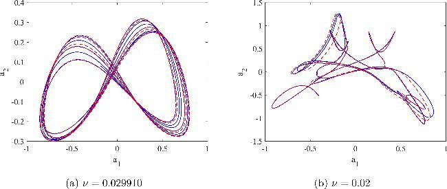
Figure 5. Phase-space projections of chaotic attractors onto the (a1, a2) plane. Blue: DNS; red: RG model. The reduced models preserve the dominant geometric structure of the respective attractors despite severe dimensionality reduction. |
In both regimes, the low-dimensional RG model preserves the essential topological features of the chaotic dynamics, demonstrating that the reduction does not destroy the characteristic organization of the phase space despite extreme dimensionality compression. The successful representation of chaotic attractors confirms that the RG method, with appropriately chosen model configurations, can scale to handle the complexity of spatiotemporal chaos.
The qualitative similarity observed in figure 5 is supported by a quantitative comparison of key dynamical measures, detailed in table 4. The table lists the mean and maximum amplitude of the dominant mode a1, along with the mean radius $\langle r\rangle =\langle \sqrt{{a}_{1}^{2}+{a}_{2}^{2}}\rangle $ in the projection plane, for both chaotic regimes.
Table 4. Characteristics of chaotic attractors at ν = 0.029 910 and ν = 0.02. |
| ν = 0.029 910 | ν = 0.02 | |||
|---|---|---|---|---|
| DNS | RG | DNS | RG | |
| Mean amplitude ⟨∣a1∣⟩ | 0.4250 | 0.4345 | 0.3524 | 0.3515 |
| Maximum ∣a1∣ | 0.8569 | 0.8573 | 0.9228 | 0.9232 |
| Mean radius $\langle r\rangle =\langle \sqrt{{a}_{1}^{2}+{a}_{2}^{2}}\rangle $ | 0.4658 | 0.5245 | 0.4984 | 0.5586 |
Comparing the values, the RG model shows high accuracy in both regimes. For ν = 0.029 910, it slightly overestimates the mean amplitude and mean radius by about 2%–3%, while matching the maximum amplitude almost exactly. In the more complex regime at ν = 0.02, it reproduces the mean amplitude with exceptional accuracy (error <0.3%) and again agrees with the maximum amplitude within 0.05%. The mean radius shows a slightly larger deviation here, consistent with the increased geometric complexity visible in figure 5(b). Together, these quantitative metrics confirm that the low-dimensional RG model captures not only the visual morphology but also the essential statistical and geometric properties of the chaotic attractors, even under severe dimensionality reduction.
In summary, the systematic validation across steady, periodic, and chaotic regimes demonstrates that the RG method successfully constructs accurate low-dimensional models for the 1D KS equation. Crucially, it achieves this not through ad-hoc fitting, but by deriving both the geometry of an approximate inertial manifold and the dynamics on it from first principles. The method balances accuracy and complexity via controllable parameters (retained modes k${}_{{\rm{\max }}}$[, truncation order), and its ability to reproduce the global bifurcation skeleton and chaotic attractor geometry confirms that the essential, long-term dynamics of the full PDE are indeed confined to a low-dimensional, RG-constructed manifold.
3.2. Two-dimensional Kuramoto–Sivashinsky equation
Following the same computational philosophy as in the 1D case, the RG framework extends naturally to the two-dimensional KS equation:
$\begin{eqnarray}{u}_{t}+{\rm{\Delta }}u+\nu {{\rm{\Delta }}}^{2}u+\frac{1}{2}| {\rm{\nabla }}u{| }^{2}=0,\end{eqnarray}$
defined on the periodic domain [0, 2π] × [0, 2π]. To maintain computational tractability while preserving rich dynamics, we restrict to even-symmetric solutions: u(t, x, y) = u(t, −x, −y). This implies Fourier coefficients satisfy a(m,n) = a(−m,−n), reducing the number of independent real amplitudes by half.The RG procedure follows the same systematic steps as in one dimension. Let ${ \mathcal K }$ denote the set of selected Fourier modes. The zeroth-order solution then takes the form:
$\begin{eqnarray}{u}_{0}(t,x,y)=\displaystyle \sum _{(m,n)\in { \mathcal K }}{a}_{(m,n)}({t}_{0}){{\rm{e}}}^{{\lambda }_{(m,n)}(t-{t}_{0})+{\rm{i}}(mx+ny)},\end{eqnarray}$
where ${\lambda }_{(m,n)}={m}^{2}+{n}^{2}-\nu {({m}^{2}+{n}^{2})}^{2}$. As in the 1D case, the truncation threshold η determines when to stop the perturbative expansion: we monitor the coefficients ${c}_{p}^{(m,n,k)}$ at each order p and truncate at order p when the largest coefficient at order p + 1 falls below η.Basis modes are selected based on linear stability: for each ν, we retain all linearly unstable modes within the circle ${m}^{2}+{n}^{2}\lt \frac{1}{\nu }$, supplemented by weakly damped stable modes needed for nonlinear saturation. Unlike the 1D case where quartic truncations were beneficial for periodic regimes, the number of resonant modal couplings grows combinatorially in two dimensions. We therefore maintain a cubic nonlinear truncation for all regimes but compensate by including a larger set of retained modes.
We employ a circular spectral truncation: the set of retained modes is {(m, n) ∈ Z2: m2 + n2 ≤ R2}, where the integer cutoff radius R satisfies $R\gt \frac{1}{\sqrt{\nu }}$ to encompass all unstable modes. Under the even-symmetry condition, the number of independent real amplitudes (excluding the zero mode) grows approximately as $\frac{\pi {R}^{2}}{2}$ for large R, reflecting the area of the spectral disk. The effectiveness of trading a higher nonlinear order for a larger spectral basis is quantified in table 5, where we see that progressively larger cutoff radii yield systematically smaller truncation errors η.
Table 5. Configuration and accuracy of 2D RG models. |
| ν | $1/\sqrt{\nu }$ | R | Number of modes | Max nonlinearity | Achieved η | |
|---|---|---|---|---|---|---|
| Fixed point | 0.51 | 1.40 | 2 | 7 | cubic (a3) | 10−2 |
| 0.51 | 1.40 | 3 | 14 | cubic (a3) | 10−4 | |
| | ||||||
| Periodic | 0.21 | 2.18 | 3 | 14 | cubic (a3) | 10−2 |
| 0.21 | 2.18 | 4 | 24 | cubic (a3) | 10−5 | |
| | ||||||
| Chaotic | 0.145 | 2.63 | 6 | 60 | cubic (a3) | 10−2 |
| 0.145 | 2.63 | 7 | 74 | cubic (a3) | 10−5 | |
R denotes the cutoff radius for the circular spectral truncation m2 + n2 ≤ R2 (the 2D analogue of kmax in 1D). Number of modes counts the number of leading Fourier modes retained in the leading-order solution u0, which equals the dimension of the reduced RG ODEs. Error indicator η is the maximum coefficient at the first omitted perturbative order. |
The visual validation in figure 6 shows u(t, x) patterns at y = π/2 for both DNS and RG models. For reference, the DNS uses 252 Fourier modes to ensure accurate resolution of the 2D dynamics. In contrast, the RG models employ only 7–74 real DOF (see table 5). For the fixed point at ν = 0.51, the reduced model with 7 real DOF perfectly reproduces the ordered stripe pattern [figure 6(a)]. In the periodic regime (ν = 0.21), a model with 24 real DOF captures both the curved stripe morphology and defect dynamics [figure 6(b)]. For weak chaos (ν = 0.145), a model with 74 real DOF generates qualitatively similar disordered patterns [figure 6(c)]. The visual match remains excellent despite these substantial reductions in the number of DOF [54].
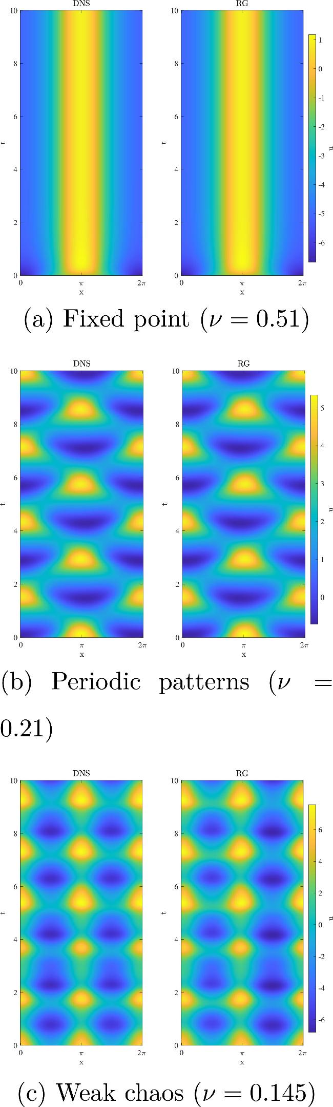


Figure 6. Spatiotemporal patterns u(t, x, y = π/2) for the 2D KS equation. Each panel shows DNS (left) alongside the corresponding RG model prediction (right). (a) Fixed point (ν = 0.51) using a model with 7 real DOF. (b) Periodic patterns (ν = 0.21) using 24 real DOF. (c) Weak chaos (ν = 0.145) using 74 real DOF. The RG models closely reproduce the characteristic patterns of each regime. |
Quantitative validation in table 6 compares maximum amplitudes of dominant modes. For the fixed point, the RG model matches DNS exactly for (1, 0) and (2, 0) modes, while correctly preserving the zero amplitude of (1, 1) (enforced by symmetry). In the periodic regime, errors are minimal: 0.08% for (1, 1) and 0.41% for (2, 0). For weak chaos, errors increase slightly but remain well controlled: 1.5% for (1, 0), 0.1% for (1, 1), and 2.6% for (2, 0). These small discrepancies are consistent with the visual impression from figure 6—the model captures essential structure while introducing minor quantitative deviations.
Table 6. Comparison of maximum modal amplitudes for 2D KS equation. Errors remain below 3% even in chaotic regimes. |
| ν (State) | Wavevector (m, n) | DNS amplitude | RG amplitude | Relative error |
|---|---|---|---|---|
| 0.51 (Fixed) | (1, 0) | 1.4645 | 1.4645 | 0.00% |
| (1, 1) | 0 | 0 | — | |
| (2, 0) | 0.2349 | 0.2349 | 0.00% | |
| | ||||
| 0.21 (Periodic) | (1, 0) | 0.0000 | 0.0038 | — |
| (1, 1) | 1.3002 | 1.2991 | 0.08% | |
| (2, 0) | 0.9659 | 0.9619 | 0.41% | |
| | ||||
| 0.145 (Weak chaos) | (1, 0) | 1.3934 | 1.4148 | 1.53% |
| (1, 1) | 0.7774 | 0.7782 | 0.10% | |
| (2, 0) | 0.7103 | 0.7288 | 2.60% | |
The application to 2D demonstrates that the RG framework retains its essential advantages with increased spatial complexity. Models with 7–74 real DOF faithfully reproduce patterns from ordered stripes to spatiotemporal chaos. This success stems from the same fundamental mechanism that worked in 1D: the RG procedure systematically integrates the effects of unresolved modes into the nonlinear couplings of retained amplitudes, effectively constructing approximate inertial manifolds. The increase in required amplitudes from 1D to 2D reflects the higher intrinsic dimensionality of the system's asymptotic dynamics, yet the relative reduction remains extreme.
The conceptual bridge between RG formalism and invariant manifold theory, which was established in section 2 and validated in 1D, proves equally robust in 2D. The RG-derived models are not ad hoc reductions but principled approximations to true inertial manifolds, constructed order by order from the governing equations. This establishes RG as a systematic and scalable pathway for dimensionality reduction in dissipative PDEs with multiple spatial dimensions.
4. Conclusion
This study demonstrates that the RG method provides a systematic and rigorous framework for constructing low-dimensional models of the KS equation. By interpreting the RG procedure as an algorithm for approximating inertial manifolds, we derive reduced systems of ordinary differential equations directly from the PDE. These models contain only a small set of real amplitudes yet accurately capture the full range of dynamics, including steady states, periodic orbits, and chaotic attractors.
Our contribution here lies in the adaptation of the finite-dimensional RG formalism to the infinite-dimensional setting of dissipative PDEs, providing a systematic perturbation algorithm for approximate inertial manifold construction that explicitly yields both the algebraic slaving relations and the reduced ODEs, as demonstrated for the KS equation.
The key advantage of this RG approach is that it is equation-driven rather than data-driven. The reduced model is derived from the fundamental equations of motion, ensuring that it inherits the correct parametric dependence and symmetry properties. This allows the model to accurately reproduce bifurcations and the subsequent period-doubling cascade to chaos. In contrast to methods that require extensive training data, the RG model remains valid in a quite large part of the parameter space.
For the one-dimensional KS equation, models with only 2–12 real DOF achieve high accuracy. In two dimensions, models with 7–74 real DOF successfully reproduce complex patterns including ordered stripes, defect dynamics, and spatiotemporal chaos. The method scales effectively to higher dimensions, though it requires careful trade-offs between the number of retained modes and the truncation order to manage computational complexity.
Despite these successes, several challenges remain. The algebraic derivation becomes increasingly complex for systems with many active modes. The current implementation relies on specific symmetry assumptions that simplify the analysis but limit generality. Mode selection, while guided by linear stability, may need refinement for problems with continuous spectra or complex nonlinear interactions.
Future work should address these limitations while extending the method to more complex systems. The structural similarities between the KS equation and the Navier–Stokes equations suggest promising applications in turbulence modeling and convective flow prediction. Developing automated software tools would make the RG approach more accessible for practical applications.
In summary, the RG method offers a principled approach to model reduction that bridges theoretical mathematics and practical computation. It provides a systematic way to extract low-dimensional dynamics from high-dimensional systems while preserving essential physical properties. While not without limitations, the method represents a significant advance in the construction of physically grounded, predictive reduced-order models.
Appendix Complete expression of u2(t, t0, x)
The full second-order correction for the N = 2 case is:
$\begin{eqnarray*}\begin{array}{rcl}{u}_{2}(t,{t}_{0},x) & = & {\rm{i}}\left(-\frac{2{a}_{1}^{3}\left({{\rm{e}}}^{3{\lambda }_{1}(t-{t}_{0})-{\rm{i}}x}-{{\rm{e}}}^{{\lambda }_{1}(t-{t}_{0})-{\rm{i}}x}\right)}{(-2+8\nu +{\lambda }_{1})(-1+\nu +3{\lambda }_{1})}\right.\\ & & +\frac{2{a}_{1}^{3}\left({{\rm{e}}}^{3{\lambda }_{1}(t-{t}_{0})+{\rm{i}}x}-{{\rm{e}}}^{{\lambda }_{1}(t-{t}_{0})+{\rm{i}}x}\right)}{(-2+8\nu +{\lambda }_{1})(-1+\nu +3{\lambda }_{1})}\\ & & -\frac{2\left({{\rm{e}}}^{{\lambda }_{1}(t-{t}_{0})+{\lambda }_{2}(t-{t}_{0})-{\rm{i}}x}-{{\rm{e}}}^{{\lambda }_{1}(t-{t}_{0})-{\rm{i}}x}\right)(-{a}_{1}^{3}+4{a}_{1}{a}_{2}^{2}+{a}_{1}^{3}\nu -16{a}_{1}{a}_{2}^{2}\nu +{a}_{1}^{3}{\lambda }_{1}-2{a}_{1}{a}_{2}^{2}{\lambda }_{1}+{a}_{1}^{3}{\lambda }_{2})}{(-2+8\nu +{\lambda }_{1}){(-1+\nu +{\lambda }_{1}+{\lambda }_{2})}^{2}}\\ & & -\frac{2\left({{\rm{e}}}^{{\lambda }_{1}(t-{t}_{0})+{\lambda }_{2}(t-{t}_{0})+{\rm{i}}x}-{{\rm{e}}}^{{\lambda }_{1}(t-{t}_{0})+{\rm{i}}x}\right)({a}_{1}^{3}-4{a}_{1}{a}_{2}^{2}-{a}_{1}^{3}\nu +16{a}_{1}{a}_{2}^{2}\nu -{a}_{1}^{3}{\lambda }_{1}+2{a}_{1}{a}_{2}^{2}{\lambda }_{1}-{a}_{1}^{3}{\lambda }_{2})}{(-2+8\nu +{\lambda }_{1}){(-1+\nu +{\lambda }_{1}+{\lambda }_{2})}^{2}}\\ & & -\frac{8{a}_{1}{a}_{2}^{2}\left({{\rm{e}}}^{{\lambda }_{1}(t-{t}_{0})+2{\lambda }_{2}(t-{t}_{0})-{\rm{i}}x}-{{\rm{e}}}^{{\lambda }_{1}(t-{t}_{0})-{\rm{i}}x}\right)(-3+39\nu -{\lambda }_{1}-{\lambda }_{2})}{(-1+\nu +{\lambda }_{1}+{\lambda }_{2})(-9+81\nu +{\lambda }_{1}+{\lambda }_{2})(-1+\nu +{\lambda }_{1}+2{\lambda }_{2})}\\ & & +\frac{8{a}_{1}{a}_{2}^{2}\left({{\rm{e}}}^{{\lambda }_{1}(t-{t}_{0})+2{\lambda }_{2}(t-{t}_{0})+{\rm{i}}x}-{{\rm{e}}}^{{\lambda }_{1}(t-{t}_{0})+{\rm{i}}x}\right)(-3+39\nu -{\lambda }_{1}-{\lambda }_{2})}{(-1+\nu +{\lambda }_{1}+{\lambda }_{2})(-9+81\nu +{\lambda }_{1}+{\lambda }_{2})(-1+\nu +{\lambda }_{1}+2{\lambda }_{2})}\\ & & -\frac{4{a}_{1}^{2}{a}_{2}\left({{\rm{e}}}^{2{\lambda }_{1}(t-{t}_{0})-2{\rm{i}}x}-{{\rm{e}}}^{{\lambda }_{2}(t-{t}_{0})-2{\rm{i}}x}\right)}{(-2+8\nu +{\lambda }_{1})(-1+\nu +{\lambda }_{1}+{\lambda }_{2})}\\ & & +\frac{4{a}_{1}^{2}{a}_{2}\left({{\rm{e}}}^{2{\lambda }_{1}(t-{t}_{0})+2{\rm{i}}x}-{{\rm{e}}}^{{\lambda }_{2}(t-{t}_{0})+2{\rm{i}}x}\right)}{(-2+8\nu +{\lambda }_{1})(-1+\nu +{\lambda }_{1}+{\lambda }_{2})}\\ & & +\frac{32{a}_{1}^{2}{a}_{2}\left({{\rm{e}}}^{2{\lambda }_{1}(t-{t}_{0})+{\lambda }_{2}(t-{t}_{0})-2{\rm{i}}x}-{{\rm{e}}}^{{\lambda }_{2}(t-{t}_{0})-2{\rm{i}}x}\right)(-3+21\nu +{\lambda }_{1}+{\lambda }_{2})}{(-1+\nu +{\lambda }_{1}+{\lambda }_{2})(-9+81\nu +{\lambda }_{1}+{\lambda }_{2})(-4+16\nu +2{\lambda }_{1}+{\lambda }_{2})}\\ & & -\frac{32{a}_{1}^{2}{a}_{2}\left({{\rm{e}}}^{2{\lambda }_{1}(t-{t}_{0})+{\lambda }_{2}(t-{t}_{0})+2{\rm{i}}x}-{{\rm{e}}}^{{\lambda }_{2}(t-{t}_{0})+2{\rm{i}}x}\right)(-3+21\nu +{\lambda }_{1}+{\lambda }_{2})}{(-1+\nu +{\lambda }_{1}+{\lambda }_{2})(-9+81\nu +{\lambda }_{1}+{\lambda }_{2})(-4+16\nu +2{\lambda }_{1}+{\lambda }_{2})}\\ & & +\frac{8{a}_{2}^{3}\left({{\rm{e}}}^{3{\lambda }_{2}(t-{t}_{0})-2{\rm{i}}x}-{{\rm{e}}}^{{\lambda }_{2}(t-{t}_{0})-2{\rm{i}}x}\right)}{(-8+128\nu +{\lambda }_{2})(-4+16\nu +3{\lambda }_{2})}\\ & & -\frac{8{a}_{2}^{3}\left({{\rm{e}}}^{3{\lambda }_{2}(t-{t}_{0})+2{\rm{i}}x}-{{\rm{e}}}^{{\lambda }_{2}(t-{t}_{0})+2{\rm{i}}x}\right)}{(-8+128\nu +{\lambda }_{2})(-4+16\nu +3{\lambda }_{2})}\\ & & -\frac{2{a}_{1}^{3}{{\rm{e}}}^{3{\lambda }_{1}(t-{t}_{0})-3{\rm{i}}x}}{(-2+8\nu +{\lambda }_{1})(-3+27\nu +{\lambda }_{1})}\\ & & +\frac{2{a}_{1}^{3}{{\rm{e}}}^{3{\lambda }_{1}(t-{t}_{0})+3{\rm{i}}x}}{(-2+8\nu +{\lambda }_{1})(-3+27\nu +{\lambda }_{1})}\\ & & -\frac{6{{\rm{e}}}^{{\lambda }_{1}(t-{t}_{0})+{\lambda }_{2}(t-{t}_{0})-3{\rm{i}}x}({a}_{1}^{3}-4{a}_{1}{a}_{2}^{2}-{a}_{1}^{3}\nu +16{a}_{1}{a}_{2}^{2}\nu -{a}_{1}^{3}{\lambda }_{1}+2{a}_{1}{a}_{2}^{2}{\lambda }_{1}-{a}_{1}^{3}{\lambda }_{2})}{(-2+8\nu +{\lambda }_{1})(-1+\nu +{\lambda }_{1}+{\lambda }_{2})(-9+81\nu +{\lambda }_{1}+{\lambda }_{2})}\\ & & -\frac{6{{\rm{e}}}^{{\lambda }_{1}(t-{t}_{0})+{\lambda }_{2}(t-{t}_{0})+3{\rm{i}}x}(-{a}_{1}^{3}+4{a}_{1}{a}_{2}^{2}+{a}_{1}^{3}\nu -16{a}_{1}{a}_{2}^{2}\nu +{a}_{1}^{3}{\lambda }_{1}-2{a}_{1}{a}_{2}^{2}{\lambda }_{1}+{a}_{1}^{3}{\lambda }_{2})}{(-2+8\nu +{\lambda }_{1})(-1+\nu +{\lambda }_{1}+{\lambda }_{2})(-9+81\nu +{\lambda }_{1}+{\lambda }_{2})}\\ & & +\frac{12{a}_{1}{a}_{2}^{2}{{\rm{e}}}^{{\lambda }_{1}(t-{t}_{0})+2{\lambda }_{2}(t-{t}_{0})-3{\rm{i}}x}(-9+129\nu +{\lambda }_{1}+2{\lambda }_{2})}{(-8+128\nu +{\lambda }_{2})(-1+\nu +{\lambda }_{1}+{\lambda }_{2})(-9+81\nu +{\lambda }_{1}+2{\lambda }_{2})}\\ & & -\frac{12{a}_{1}{a}_{2}^{2}{{\rm{e}}}^{{\lambda }_{1}(t-{t}_{0})+2{\lambda }_{2}(t-{t}_{0})+3{\rm{i}}x}(-9+129\nu +{\lambda }_{1}+2{\lambda }_{2})}{(-8+128\nu +{\lambda }_{2})(-1+\nu +{\lambda }_{1}+{\lambda }_{2})(-9+81\nu +{\lambda }_{1}+2{\lambda }_{2})}\\ & & +\frac{4{a}_{1}^{2}{a}_{2}{{\rm{e}}}^{2{\lambda }_{2}(t-{t}_{0})-4{\rm{i}}x}}{(-2+8\nu +{\lambda }_{1})(-8+128\nu +{\lambda }_{2})}\\ & & -\frac{4{a}_{1}^{2}{a}_{2}{{\rm{e}}}^{2{\lambda }_{2}(t-{t}_{0})+4{\rm{i}}x}}{(-2+8\nu +{\lambda }_{1})(-8+128\nu +{\lambda }_{2})}\\ & & -\frac{8{a}_{1}^{2}{a}_{2}{{\rm{e}}}^{2{\lambda }_{1}(t-{t}_{0})+{\lambda }_{2}(t-{t}_{0})-4{\rm{i}}x}(-21+129\nu +7{\lambda }_{1}+{\lambda }_{2})}{(-2+8\nu +{\lambda }_{1})(-9+81\nu +{\lambda }_{1}+{\lambda }_{2})(-16+256\nu +2{\lambda }_{1}+{\lambda }_{2})}\\ & & +\frac{8{a}_{1}^{2}{a}_{2}{{\rm{e}}}^{2{\lambda }_{1}(t-{t}_{0})+{\lambda }_{2}(t-{t}_{0})+4{\rm{i}}x}(-21+129\nu +7{\lambda }_{1}+{\lambda }_{2})}{(-2+8\nu +{\lambda }_{1})(-9+81\nu +{\lambda }_{1}+{\lambda }_{2})(-16+256\nu +2{\lambda }_{1}+{\lambda }_{2})}\\ & & -\frac{20{a}_{1}{a}_{2}^{2}{{\rm{e}}}^{{\lambda }_{1}(t-{t}_{0})+2{\lambda }_{2}(t-{t}_{0})-5{\rm{i}}x}(-33+465\nu +{\lambda }_{1}+4{\lambda }_{2})}{(-8+128\nu +{\lambda }_{2})(-9+81\nu +{\lambda }_{1}+{\lambda }_{2})(-25+625\nu +{\lambda }_{1}+2{\lambda }_{2})}\\ & & +\frac{20{a}_{1}{a}_{2}^{2}{{\rm{e}}}^{{\lambda }_{1}(t-{t}_{0})+2{\lambda }_{2}(t-{t}_{0})+5{\rm{i}}x}(-33+465\nu +{\lambda }_{1}+4{\lambda }_{2})}{(-8+128\nu +{\lambda }_{2})(-9+81\nu +{\lambda }_{1}+{\lambda }_{2})(-25+625\nu +{\lambda }_{1}+2{\lambda }_{2})}\\ & & -\frac{8{a}_{2}^{3}{{\rm{e}}}^{3{\lambda }_{2}(t-{t}_{0})-6{\rm{i}}x}}{(-8+128\nu +{\lambda }_{2})(-12+432\nu +{\lambda }_{2})}\left.+\frac{8{a}_{2}^{3}{{\rm{e}}}^{3{\lambda }_{2}(t-{t}_{0})+6{\rm{i}}x}}{(-8+128\nu +{\lambda }_{2})(-12+432\nu +{\lambda }_{2})}\right).\end{array}\end{eqnarray*}$