Welcome to visit Communications in Theoretical Physics,
Mathematical Physics

Inverse scattering transform of the focusing Lakshmanan–Porsezian–Daniel equation with one-sided nonzero boundary condition

  • Feng Zhang ,
  • Pengfei Han ,
  • Yi Zhang ,
Expand
  • School of Mathematical Sciences, Zhejiang Normal University, Jinhua 321004, China

Author to whom any correspondence should be addressed.

Received date: 2025-12-21

  Revised date: 2026-03-26

  Accepted date: 2026-03-27

  Online published: 2026-05-01

Copyright

© 2026 Institute of Theoretical Physics CAS, Chinese Physical Society and IOP Publishing. All rights, including for text and data mining, AI training, and similar technologies, are reserved.
This article is available under the terms of the IOP-Standard License.

Abstract

In this study, we develop the inverse scattering transform of the focusing Lakshmanan–Porsezian–Daniel equation with a one-sided nonzero boundary condition, where the asymptotic amplitude tends to zero on one side at spatial infinity while remaining nonzero on the other. For the direct scattering problem, single-valued eigenfunctions are rigorously defined, and their analyticity, symmetries, and asymptotic behavior are rigorously analyzed. Furthermore, the Marchenko integral equations and the Riemann–Hilbert problems (both right and left) on a single sheet of the scattering variable are constructed and utilized to formulate the inverse problem. Additionally, a proper uniformization variable is defined to formulate both the direct and inverse scattering problems, which maps the two-sheeted Riemann surface of the spectral parameter onto a single complex plane. Ultimately, the time evolutions of the eigenfunctions are derived, revealing the nontrivial time dependence of the scattering data.

Cite this article

Feng Zhang , Pengfei Han , Yi Zhang . Inverse scattering transform of the focusing Lakshmanan–Porsezian–Daniel equation with one-sided nonzero boundary condition[J]. Communications in Theoretical Physics, 2026 , 78(7) : 075003 . DOI: 10.1088/1572-9494/ae5802

1. Introduction

Since the inverse scattering transform (IST) method was first successfully applied to solve the KdV equation [1], this groundbreaking technique has been rapidly extended to numerous integrable nonlinear evolution equations [26]. Among these integrable systems, the nonlinear Schrödinger (NLS) equation occupies a central position due to its rich physical significance. As a universal model of wave propagation under weakly nonlinear and weakly dispersive conditions [7, 8], the NLS equation has been widely utilized in diverse fields, including Bose–Einstein condensation, nonlinear optics, plasma physics, and biological systems [911]. In 1972, Zakharov and Shabat pioneered the construction of the IST theoretical framework for the NLS equation [12], achieving soliton solutions for the first time via the scattering problem for Lax pair, and further extending the method to nonzero boundary conditions (NZBC) [13]. Subsequent research by Ablowitz, Biondini, and others has further refined this theoretical foundation [1417], solidifying it as a cornerstone for studying multi-soliton interactions, modulation instability, and energy conservation in the NLS equation. However, as research into complex physical phenomena such as deep ocean waves and ultrafast laser pulses progresses, the classical NLS equation has been found insufficient to describe higher-order dispersion effects and nonlinear coupling mechanisms, necessitating its higher-order generalizations [1821]. The Lakshmanan–Porsezian–Daniel (LPD) equation has emerged as a significant higher-order extended model, effectively capturing fourth-order dispersion effects and more complex nonlinear interactions. It holds considerable importance in describing higher-order nonlinear wave dynamics and is completely integrable [2224].
This paper investigates the focusing LPD equation
$\begin{eqnarray}\begin{array}{rcl} & & {\rm{i}}{u}_{t}+{u}_{xx}+2{\left|u\right|}^{2}u+\gamma \left({u}_{xxxx}+4{\left|{u}_{x}\right|}^{2}u+6{u}_{x}^{2}{u}^{* }\right.\\ & & \,\left.+8{u}_{xx}{\left|u\right|}^{2}+2{u}^{2}{u}_{xx}^{* }+6{\left|u\right|}^{4}u\right)=0,\end{array}\end{eqnarray}$
where the complex-valued function $u=u(t,x)$ characterizes the spatiotemporal evolution of the wave packet, and the real parameter γ quantifies the fourth-order dispersion effect and the corresponding higher-order nonlinear coupling strength [25]. When γ = 0, it recovers the classical NLS equation. The LPD equation is of considerable physical relevance due to its capacity to model wave propagation in systems with prominent higher-order nonlinearity and dispersion coupling. It proves especially effective in capturing nonlinear effects that are not covered by the standard NLS equation [22, 26, 27]. For example, during the propagation of ultrashort optical pulses, the introduction of fourth-order dispersion and higher-order nonlinear terms enables a more precise reflection of the pulse evolution characteristics within strongly dispersive media, providing a more comprehensive description of pulse shape and spectral changes [18, 23, 28, 29]. Moreover, the LPD equation plays a significant role in magnetic system modeling, where it extends the classical Landau–Lifshitz equation by incorporating octupole-dipole interactions and anisotropic higher-order exchange effects [25, 30]. It thus provides an effective tool for studying nonlinear spin waves and magnetic soliton dynamics in ferromagnetic materials. Owing to its capacity for handling higher-order dispersion, nonlinear coupling, and complex material effects, the study of the LPD equation is of significant theoretical value for advancing our understanding of nonlinear wave propagation in optical and magnetic media.
As an important integrable model, the LPD equation has been extensively studied in mathematical physics [31, 32], with its rich solution structures (including solitons, breathers and rogue waves) systematically explored through modern integrable theory tools such as the IST, the Riemann–Hilbert (RH) method, etc. Under zero boundary condition, the IST of the LPD equation was thoroughly investigated in [33], where multi-soliton and higher-order soliton solutions were constructed. In [34], the RH method was employed to study its multi-coupled form, while [35] examined the three-coupled form, discussing the long time asymptotics for the Schwartz initial value problem. Under NZBC [36, 37], studied the IST of both the focusing and defocusing LPD equation, constructing single and double pole solutions. A robust IST for this equation was proposed in [38], where the breather and rogue wave solutions were derived. In subsequent studies [39], the IST framework for the LPD equation with NZBC was extended to its two-component vector form. It should be noted that existing research has primarily focused on symmetric NZBC, that is, the modulus of the solution and the vector norms all approach the same value as the spatial coordinate tends to infinity. However, in practical applications, such symmetric NZBC are restrictive, as the background amplitudes at both spatial infinities often differ in many physical systems.
This study aims to develop the IST for the focusing LPD equation (1.1), particularly with the one-sided NZBC
$\begin{eqnarray}\begin{array}{l}u\left(t,x\right)\to 0,x\to -\infty \\ u\left(t,x\right)\to {u}_{r}\left(t\right)={\alpha }_{r}{{\rm{e}}}^{2{\rm{i}}{\alpha }_{r}^{2}(1+3\gamma {\alpha }_{r}^{2})t+{\rm{i}}{\nu }_{r}},\\ x\to +\infty ,\end{array}\end{eqnarray}$
where 0 ≤ νr < 2π and αr > 0 are arbitrary constants. The fully asymmetric NZBC refers to the case where the asymptotic phases as well as amplitudes are asymmetric in space, which was first proposed by Demontis, Prinari et al. They developed the IST for the focusing NLS equation with this boundary condition [40]. Shortly thereafter, Biondini extended this framework to the defocusing case [41]. Evidently, the one-sided NZBC discussed above transcends the scope of the same amplitudes explored in [16, 36], representing a special kind of asymmetric scenario. Similar to the symmetric NZBC, under condition (1.2), a uniformization variable can be introduced, a process that is infeasible under the fully asymmetric NZBC. However, in contrast to symmetric NZBC, significant differences remain in addressing both the direct and inverse problems. Moreover, it is important to note that degeneration from the fully asymmetric NZBC to the corresponding results is not possible. Therefore, the case of one-sided NZBC warrants separate study. From the perspectives of both physics and practical applications, extending the symmetric NZBC to the one-sided NZBC is highly significant. It provides an essential theoretical model for directed propagation of nonlinear waves in media, energy transport, and interactions with background fields. In nonlinear optics, the one-sided NZBC corresponds to single-end pumped fiber systems, facilitating the study of the asymptotic behavior of optical pulses propagating unidirectionally in fibers and advancing theoretical research on rogue waves and perturbed solitons propagating in microstructured fibers characterized by asymmetric background amplitudes at their terminals [42]. Constructing the IST of the focusing LPD equation with boundary condition (1.2) will help illuminate the crucial role of soliton dynamics in the nonlinear evolution of modulation instability in integrable systems [43].
The structure of this article is as follows. In section 2, the direct problem is thoroughly examined. The Volterra integral equations are established, and the analytic properties of the eigenfunctions and scattering coefficients are deduced. In addition, two sets of symmetries for the scattering data, as well as their asymptotic behavior are established. In section 3, we formulate the inverse problem using both right and left Marchenko integral equations and matrix RH problems, and reconstruct the potential function via the Marchenko kernels and the solutions of the RH problems. In both formulations of the inverse problem, additional spectral data on the oriented contours contribute nontrivially to the corresponding integral terms, in addition to the continuous spectrum and the discrete eigenvalues of the scattering problem. Therefore, unlike the symmetric NZBC case treated in [16, 36], it is not feasible to reformulate the inverse problem as a set of algebraic equations via the reflectionless condition and then derive explicit solutions, indicating the absence of purely soliton solutions under one-sided NZBC. In section 4, the time evolution equations of the eigenfunctions and other scattering data are determined through the introduced time-dependent exponential functions, demonstrating their significant temporal dependence. In section 5, we define a uniformization variable z and discuss the direct as well as inverse scattering problems on a single complex z-plane. Section 6 summarizes and discusses the findings of this paper.

2. Direct problem

The Lax pair for the focusing LPD equation (1.1) is given by [25]
$\begin{eqnarray}{{\boldsymbol{\phi }}}_{x}={\boldsymbol{X}}\left(t,x,\lambda \right){\boldsymbol{\phi }},\end{eqnarray}$
$\begin{eqnarray}{{\boldsymbol{\phi }}}_{t}={\boldsymbol{T}}\left(t,x,\lambda \right){\boldsymbol{\phi }},\end{eqnarray}$
where φ = φ(λtx) is an eigenfunction, $\lambda \in {\mathbb{C}}$ represents the spectral parameter, and
$\begin{eqnarray*}\begin{array}{rcl}{\boldsymbol{X}} & = & -{\rm{i}}\lambda {{\boldsymbol{\sigma }}}_{3}+{\boldsymbol{U}},\\ {\boldsymbol{T}} & = & -2{\rm{i}}{\lambda }^{2}{{\boldsymbol{\sigma }}}_{3}+2\lambda {\boldsymbol{U}}+{\rm{i}}{{\boldsymbol{\sigma }}}_{3}\left({{\boldsymbol{U}}}_{x}-{{\boldsymbol{U}}}^{2}\right)\\ & & +\gamma \left[8{\rm{i}}{\lambda }^{4}{{\boldsymbol{\sigma }}}_{3}-8{\lambda }^{3}{\boldsymbol{U}}-4{\rm{i}}{\lambda }^{2}{{\boldsymbol{\sigma }}}_{3}\left({{\boldsymbol{U}}}_{x}-{{\boldsymbol{U}}}^{2}\right)-2\lambda \left({{\boldsymbol{U}}}_{x}{\boldsymbol{U}}-{\boldsymbol{U}}{{\boldsymbol{U}}}_{x}\right)\right]\\ & & -\gamma \left[2\lambda \left(2{{\boldsymbol{U}}}^{3}-{{\boldsymbol{U}}}_{xx}\right)+3{\rm{i}}{{\boldsymbol{\sigma }}}_{3}\left({{\boldsymbol{U}}}_{x}{{\boldsymbol{U}}}^{2}+{{\boldsymbol{U}}}^{2}{{\boldsymbol{U}}}_{x}-{{\boldsymbol{U}}}^{4}\right)\right.\\ & & \left.+{\rm{i}}{{\boldsymbol{\sigma }}}_{3}\left({{\boldsymbol{U}}}_{xx}{\boldsymbol{U}}+{\boldsymbol{U}}{{\boldsymbol{U}}}_{xx}\right)-{\rm{i}}{{\boldsymbol{\sigma }}}_{3}\left({{\boldsymbol{U}}}_{xxx}+{{\boldsymbol{U}}}_{x}^{2}\right)\right],\\ {\boldsymbol{U}} & = & \left(\begin{array}{cc}0 & u\\ -{u}^{* } & 0\end{array}\right),{{\boldsymbol{\sigma }}}_{3}=\left(\begin{array}{cc}1 & 0\\ 0 & -1\end{array}\right),\\ {{\boldsymbol{\sigma }}}_{2} & = & \left(\begin{array}{cc}0 & -{\rm{i}}\\ {\rm{i}} & 0\end{array}\right),{{\boldsymbol{\sigma }}}_{1}=\left(\begin{array}{cc}0 & 1\\ 1 & 0\end{array}\right).\end{array}\end{eqnarray*}$
In the following, we consider the u(t, x) with a one-sided NZBC (1.2), where the asymptotic phase is given by ${\nu }_{r}\left(t\right)=2{\alpha }_{r}^{2}(1+3\gamma {\alpha }_{r}^{2})t+{\nu }_{r}$, and the asymptotic amplitude αr > 0 is a time-independent constant. A key distinction from the symmetric NZBC case [16, 36] is the inapplicability of the rescaling $u=\hat{u}{{\rm{e}}}^{2{\rm{i}}{u}_{o}^{2}(1+3\gamma {u}_{o}^{2})t}$ to eliminate the boundary condition's time dependence. In addition, for t ≥ 0, we introduce an integrability condition
$\begin{eqnarray}({{\boldsymbol{L}}}_{\iota }):{\int }_{-\infty }^{\infty }\left|u(t,x)-h(x){u}_{r}(t)\right|{\left(1+\left|x\right|\right)}^{\iota }{\rm{d}}x\lt \infty ,\end{eqnarray}$
where h(x) denotes the Heaviside function and ι = 0, 1.
To facilitate the presentation of the direct problem in this section, the explicit time dependence is now omitted. Based on the boundary condition (1.2), we represent the limit value of U(tx) as x → + by Ur(t), and U(tx) → 0 as x → −, where 0 is a 2 × 2 zero matrix. The asymptotic scattering operators as x → + are defined to be
$\begin{eqnarray*}{{\boldsymbol{X}}}_{r}\left(\lambda \right)=-{\rm{i}}\lambda {{\boldsymbol{\sigma }}}_{3}+{{\boldsymbol{U}}}_{r},\tilde{{\boldsymbol{X}}}\left(x,\lambda \right)=-{\rm{i}}\lambda {{\boldsymbol{\sigma }}}_{3}+\tilde{{\boldsymbol{U}}},\end{eqnarray*}$
where $\tilde{{\boldsymbol{U}}}=h(x){{\boldsymbol{U}}}_{r}(t)$ is free potential matrix. In the following, we suppose that ${\boldsymbol{Q}}\left(x,\lambda \right)$ denotes the eigenfunction and $\tilde{{\boldsymbol{P}}}\left(x,\lambda \right)$ denotes the matrix fundamental eigensolution, which are solutions of (2.1). Their asymptotic conditions are given by
$\begin{eqnarray}\begin{array}{l}\tilde{{\boldsymbol{P}}}\left(x,\lambda \right)={{\rm{e}}}^{{{\boldsymbol{X}}}_{r}\left(\lambda \right)x}\left({\boldsymbol{I}}+o\left(1\right)\right),x\to +\infty ,\\ {\boldsymbol{Q}}\left(x,\lambda \right)={{\rm{e}}}^{-{\rm{i}}\lambda {{\boldsymbol{\sigma }}}_{3}x}\left({\boldsymbol{I}}+o\left(1\right)\right),x\to -\infty ,\end{array}\end{eqnarray}$
where I is defined as the 2 × 2 identity matrix.
Introduce the following notations:
$\begin{eqnarray*}{{\rm{\Theta }}}_{r}=\left[-{\rm{i}}{\alpha }_{r},{\rm{i}}{\alpha }_{r}\right],{{\rm{\Theta }}}_{r}^{+}=\left[0,{\rm{i}}{\alpha }_{r}\right],{{\rm{\Theta }}}_{r}^{-}=\left[-{\rm{i}}{\alpha }_{r},0\right],\end{eqnarray*}$
with their respective interiors denoted by
$\begin{eqnarray*}{\mathop{{\rm{\Theta }}}\limits^{\circ }}_{r}=\left(-{\rm{i}}{\alpha }_{r},{\rm{i}}{\alpha }_{r}\right),{\mathop{{\rm{\Theta }}}\limits^{\circ }}_{r}^{+}=\left(0,{\rm{i}}{\alpha }_{r}\right),{\mathop{{\rm{\Theta }}}\limits^{\circ }}_{r}^{-}=\left(-{\rm{i}}{\alpha }_{r},0\right).\end{eqnarray*}$
Suppose the integrability condition (L0) holds for the potential function. The eigensolution $\tilde{{\boldsymbol{P}}}\left(x,\lambda \right)$ and eigenfunction ${\boldsymbol{Q}}\left(x,\lambda \right)$ are uniquely constructed via the following integral equations:
$\begin{eqnarray}\begin{array}{r}\tilde{{\boldsymbol{P}}}\left(x,\lambda \right)={{\rm{e}}}^{{{\boldsymbol{X}}}_{r}\left(\lambda \right)x}+{\displaystyle \int }_{\infty }^{x}{{\rm{e}}}^{\left(x-\zeta \right){{\boldsymbol{X}}}_{r}(\lambda )}{\rm{\Delta }}{{\boldsymbol{U}}}_{r}\left(\zeta \right)\tilde{{\boldsymbol{P}}}\left(\zeta ,\lambda \right){\rm{d}}\zeta ,\\ \lambda \in {\mathbb{R}}\cup {\mathop{{\rm{\Theta }}}\limits^{\circ }}_{r},\end{array}\end{eqnarray}$
$\begin{eqnarray}\begin{array}{r}{\boldsymbol{Q}}\left(x,\lambda \right)={{\rm{e}}}^{-{\rm{i}}\lambda {{\boldsymbol{\sigma }}}_{3}x}+{\displaystyle \int }_{-\infty }^{x}{{\rm{e}}}^{{\rm{i}}\lambda \left(\zeta -x\right){{\boldsymbol{\sigma }}}_{3}}{\boldsymbol{U}}\left(\zeta \right){\boldsymbol{Q}}\left(\zeta ,\lambda \right){\rm{d}}\zeta ,\\ \lambda \in {\mathbb{R}},\end{array}\end{eqnarray}$
where ${\rm{\Delta }}{{\boldsymbol{U}}}_{r}\left(\zeta \right)={\boldsymbol{U}}\left(\zeta \right)-{{\boldsymbol{U}}}_{r}$. Furthermore, $\tilde{{\boldsymbol{P}}}\left(x,\lambda \right)$ is continuous for xxo (any finite xo), and regarded as a function of λ, remains continuous for $\lambda \in {\mathbb{R}}\cup {\mathop{{\rm{\Theta }}}\limits^{\circ }}_{r}$. Meanwhile, ${\boldsymbol{Q}}\left(x,\lambda \right)$ is continuous in $x\in {\mathbb{R}}$ for every $\lambda \in {\mathbb{R}}$. Notice that if the potential function satisfies the integrability condition (L1), the integral equation (2.5) has a continuous solution $\tilde{{\boldsymbol{P}}}\left(x,\lambda \right)$ for every λ ∈ Θr.
A fundamental matrix function ${\boldsymbol{H}}\left(\lambda ,\zeta ,x\right)$ is introduced as
$\begin{eqnarray}\begin{array}{rcl}{\boldsymbol{H}}\left(\lambda ,\zeta ,x\right) & = & h\left(\zeta \right)h\left(x\right){{\rm{e}}}^{\left(x-\zeta \right){{\boldsymbol{X}}}_{r}\left(\lambda \right)}\\ & & +h\left(-\zeta \right)h\left(-x\right){{\rm{e}}}^{-{\rm{i}}\lambda (x-\zeta ){{\boldsymbol{\sigma }}}_{3}}\\ & & +h\left(-\zeta \right)h\left(x\right){{\rm{e}}}^{{{\boldsymbol{X}}}_{r}\left(\lambda \right)x}{{\rm{e}}}^{{\rm{i}}\lambda {{\boldsymbol{\sigma }}}_{3}\zeta }\\ & & +h\left(\zeta \right)h\left(-x\right){{\rm{e}}}^{-{\rm{i}}\lambda {{\boldsymbol{\sigma }}}_{3}x}{{\rm{e}}}^{-{{\boldsymbol{X}}}_{r}\left(\lambda \right)\zeta },\\ & & \zeta ,x\in {\mathbb{R}},\lambda \in {\mathbb{C}},\end{array}\end{eqnarray}$
with the initial value conditions
$\begin{eqnarray}\begin{array}{l}{\partial }_{x}{\boldsymbol{H}}\left(\lambda ,\zeta ,x\right)=\tilde{{\boldsymbol{X}}}\left(x,\lambda \right){\boldsymbol{H}}\left(\lambda ,\zeta ,x\right),\\ {\boldsymbol{H}}\left(\lambda ,\zeta ,\zeta \right)={\boldsymbol{I}},\\ {\partial }_{\zeta }{\boldsymbol{H}}\left(\lambda ,\zeta ,x\right)=-{\boldsymbol{H}}\left(\lambda ,\zeta ,x\right)\tilde{{\boldsymbol{X}}}\left(x,\lambda \right),\\ {\boldsymbol{H}}\left(\lambda ,x,x\right)={\boldsymbol{I}}.\end{array}\end{eqnarray}$
Setting ζ = 0, we have
$\begin{eqnarray*}\begin{array}{l}{\boldsymbol{H}}\left(\lambda ,0,x\right)=h\left(x\right){{\rm{e}}}^{{{\boldsymbol{X}}}_{r}\left(\lambda \right)x}+h\left(-x\right){{\rm{e}}}^{-{\rm{i}}\lambda {{\boldsymbol{\sigma }}}_{3}x}.\end{array}\end{eqnarray*}$
Analysis of the initial value problems (2.8) indicates that $\tilde{{\boldsymbol{P}}}\left(x,\lambda \right)$, ${\boldsymbol{Q}}\left(x,\lambda \right)$ satisfy the integral equations
$\begin{eqnarray}\begin{array}{rcl}\tilde{{\boldsymbol{P}}}\left(x,\lambda \right) & = & {\boldsymbol{H}}\left(\lambda ,0,x\right)\\ & & -{\displaystyle \int }_{x}^{\infty }{\boldsymbol{H}}\left(\lambda ,\zeta ,x\right){\rm{\Delta }}\tilde{{\boldsymbol{U}}}\left(\zeta \right)\tilde{{\boldsymbol{P}}}\left(\zeta ,\lambda \right){\rm{d}}\zeta ,\end{array}\end{eqnarray}$
$\begin{eqnarray}\begin{array}{l}{\boldsymbol{Q}}\left(x,\lambda \right)\,=\,{\boldsymbol{H}}\left(\lambda ,0,x\right)\\ \,+{\displaystyle \int }_{-\infty }^{x}{\boldsymbol{H}}\left(\lambda ,\zeta ,x\right){\rm{\Delta }}\tilde{{\boldsymbol{U}}}\left(\zeta \right){\boldsymbol{Q}}\left(\zeta ,\lambda \right){\rm{d}}\zeta ,\end{array}\end{eqnarray}$
where ${\rm{\Delta }}\tilde{{\boldsymbol{U}}}(\zeta )={\boldsymbol{U}}(\zeta )-\tilde{{\boldsymbol{U}}}(\zeta )$. A direct comparison reveals that equation (2.9) reduces to equation (2.5) for x ≥ 0, while equation (2.10) coincides with equation (2.6) for x ≤ 0. By substituting ${\boldsymbol{H}}\left(\lambda ,x,\zeta \right)$ into these integral equations, the system is transformed into an equivalent system defined by equations
$\begin{eqnarray}\begin{array}{l}{{\rm{e}}}^{{\rm{i}}\lambda {{\boldsymbol{\sigma }}}_{3}x}\tilde{{\boldsymbol{P}}}\left(x,\lambda \right)={\boldsymbol{I}}-{\displaystyle \int }_{x}^{\infty }{\boldsymbol{H}}\left(\lambda ,\zeta ,0\right){\rm{\Delta }}\tilde{{\boldsymbol{U}}}\left(\zeta \right)\tilde{{\boldsymbol{P}}}\left(\zeta ,\lambda \right){\rm{d}}\zeta ,\\ {{\rm{e}}}^{-{{\boldsymbol{X}}}_{r}\left(\lambda \right)x}{\boldsymbol{Q}}\left(x,\lambda \right)={\boldsymbol{I}}+{\displaystyle \int }_{-\infty }^{x}{\boldsymbol{H}}\left(\lambda ,\zeta ,0\right){\rm{\Delta }}\tilde{{\boldsymbol{U}}}\left(\zeta \right){\boldsymbol{Q}}\left(\zeta ,\lambda \right){\rm{d}}\zeta .\end{array}\end{eqnarray}$

2.1. Jost solutions

It is easy to verify that ${\rm{Tr}}{{\boldsymbol{X}}}_{r}(\lambda )=0$, and ${{\boldsymbol{X}}}_{r}^{2}(\lambda )\,=-({\lambda }^{2}+{\alpha }_{r}^{2}){\boldsymbol{I}}$, which requires us to construct a two-sheeted Riemann surface related to ${\chi }_{r}^{2}={\lambda }^{2}+{\alpha }_{r}^{2}$ by defining the local polar coordinate on Sheet 1 is ${\chi }_{r}=\sqrt{{a}_{1}{a}_{2}}{{\rm{e}}}^{{\rm{i}}\left({\nu }_{1}+{\nu }_{2}\right)/2}$, on Sheet 2 is ${\chi }_{r}=-\sqrt{{a}_{1}{a}_{2}}{{\rm{e}}}^{{\rm{i}}\left({\nu }_{1}+{\nu }_{2}\right)/2}$, and the branching cut is Θr, where −π/2 ≤ νk < 3π/2, ak ≥ 0, (k = 1, 2).
In the following, we will only consider a single sheet (Sheet 1) of the complex λ-plane, and the symbol ${{\mathbb{D}}}_{r}$ is defined as the plane cut along the Θr. This domain is decomposed as follows
$\begin{eqnarray*}\begin{array}{l}{{\mathbb{D}}}_{r}^{-}={{\mathbb{C}}}^{-}\backslash \left[-{\rm{i}}{\alpha }_{r},0\right),{{\mathbb{D}}}_{r}^{+}={{\mathbb{C}}}^{+}\backslash \left(0,{\rm{i}}{\alpha }_{r}\right],\\ \partial {{\mathbb{D}}}_{r}^{\pm }={\mathbb{R}}\cup \left\{\pm {\rm{i}}{d}_{r}-{0}^{+}\right\}\cup \left\{\pm {\rm{i}}{\alpha }_{r}\right\}\cup \left\{\pm {\rm{i}}{d}_{r}+{0}^{+}\right\},\end{array}\end{eqnarray*}$
where dr is an arbitrary constant satisfying 0 < dr < αr, $\partial {{\mathbb{D}}}_{r}^{\pm }$ is the boundary of ${{\mathbb{D}}}_{r}^{\pm }$. The mapping χr is bijective from the interior points $\lambda \in {{\mathbb{D}}}_{r}^{\pm }$ to ${\chi }_{r}\in {{\mathbb{C}}}^{\pm }$, while it maps the boundary $\lambda \in \partial {{\mathbb{D}}}_{r}^{\pm }$ bijectively onto ${\chi }_{r}\in {\mathbb{R}}$. Moreover, we note that this branch cut is chosen such that χr ∼ λ as λ →  in Sheet 1, while χr ∼ − λ as λ →  on Sheet 2. Next, we utilize ${\chi }_{r}^{\pm }(\lambda )$ to represent the boundary values of χr on the right/left edge of Θr on Sheet 1, i.e.
$\begin{eqnarray}{\chi }_{r}^{\pm }\left(\lambda \right)=\pm \sqrt{{\alpha }_{r}^{2}-{\left|\lambda \right|}^{2}},\lambda ={\rm{i}}{d}_{r}\pm {0}^{+}.\end{eqnarray}$
The eigenvalue matrix ωr(λ) and eigenvector matrix ϖr(λ) of ${{\boldsymbol{X}}}_{r}\left(\lambda \right)$ are obtained through direct calculation as
$\begin{eqnarray*}\begin{array}{l}{{\boldsymbol{\omega }}}_{r}(\lambda )={\rm{diag}}\left(-{\rm{i}}{\chi }_{r},{\rm{i}}{\chi }_{r}\right),{{\boldsymbol{\varpi }}}_{r}(\lambda )={\boldsymbol{I}}-\frac{{\rm{i}}}{\lambda +{\chi }_{r}}{{\boldsymbol{\sigma }}}_{3}{{\boldsymbol{U}}}_{r},\end{array}\end{eqnarray*}$
and they satisfy the below relation
$\begin{eqnarray*}{{\boldsymbol{X}}}_{r}\left(\lambda \right)={{\boldsymbol{\varpi }}}_{r}(\lambda ){{\boldsymbol{\omega }}}_{r}(\lambda ){{\boldsymbol{\varpi }}}_{r}^{-1}(\lambda ).\end{eqnarray*}$
Here, ϖr(λ) is not a singular matrix on either sheet since αr > 0 holds strictly (χr + λ only vanish on Sheet 2 as λ → ) and there is ${\rm{\det }}{{\boldsymbol{\varpi }}}_{r}(\lambda )=\frac{2{\chi }_{r}}{{\chi }_{r}+\lambda }$.
The right Jost solution ${\boldsymbol{P}}\left(x,\lambda \right)$ is constructed from the fundamental eigensolution $\tilde{{\boldsymbol{P}}}\left(x,\lambda \right)$ via the relation
$\begin{eqnarray*}\begin{array}{l}{\boldsymbol{P}}\left(x,\lambda \right)=\left(\tilde{p}(x,\lambda ),p(x,\lambda )\right)=\tilde{{\boldsymbol{P}}}\left(x,\lambda \right){{\boldsymbol{\varpi }}}_{r}\left(\lambda \right),\end{array}\end{eqnarray*}$
which likewise satisfies the spatial spectral problem (2.1). Furthermore, its asymptotic behavior as x → + is obtained from equation (2.4) as
$\begin{eqnarray}\begin{array}{l}{\boldsymbol{P}}\left(x,\lambda \right)={{\boldsymbol{\varpi }}}_{r}\left(\lambda \right){{\rm{e}}}^{-{\rm{i}}{\chi }_{r}{{\boldsymbol{\sigma }}}_{3}x}\left({\boldsymbol{I}}+o\left(1\right)\right),x\to +\infty .\end{array}\end{eqnarray}$
According to equation (2.12), ϖr(λ) has right and left limits and $\tilde{{\boldsymbol{P}}}\left(x,\lambda \right)$ crosses Θr as a single-valued function, so we can utilize ${{\boldsymbol{P}}}^{\pm }\left(x,{\rm{i}}{d}_{r}\right)$ to represent the limit values of the Jost solution ${\boldsymbol{P}}\left(x,\lambda \right)$ at the right/left edge of Θr, i.e.
$\begin{eqnarray*}\begin{array}{l}{{\boldsymbol{P}}}^{\pm }\left(x,{\rm{i}}{d}_{r}\right)=\left({\tilde{p}}^{\pm }\left(x,{\rm{i}}{d}_{r}\right),{p}^{\pm }\left(x,{\rm{i}}{d}_{r}\right)\right)\\ =\,\tilde{{\boldsymbol{P}}}\left(x,{\rm{i}}{d}_{r}\right){{\boldsymbol{\varpi }}}_{r}\left({\rm{i}}{d}_{r}\pm {0}^{+}\right),{\rm{i}}{d}_{r}\in {{\rm{\Theta }}}_{r}.\end{array}\end{eqnarray*}$
Combining equations (2.5) and (2.6) with the identity ${{\rm{e}}}^{{{\boldsymbol{X}}}_{r}\left(\lambda \right)x}={{\boldsymbol{\varpi }}}_{r}\left(\lambda \right){{\rm{e}}}^{{{\boldsymbol{\omega }}}_{r}(\lambda )x}{{\boldsymbol{\varpi }}}_{r}^{-1}\left(\lambda \right)$, the Jost solutions can be represented by the Volterra integral equations:
$\begin{eqnarray}\begin{array}{c}\,{{\rm{e}}}^{{\rm{i}}{\chi }_{r}x}\tilde{p}(x,\lambda )={{\boldsymbol{\varpi }}}_{r,1}(\lambda )-{\displaystyle \int }_{x}^{+\infty }{{\boldsymbol{E}}}_{r}^{-}\left(\zeta -x,\lambda \right){\rm{\Delta }}{{\boldsymbol{U}}}_{r}{{\rm{e}}}^{{\rm{i}}{\chi }_{r}\zeta }\tilde{p}\left(\zeta ,\lambda \right)\,{\rm{d}}\zeta ,\\ \,{{\rm{e}}}^{-{\rm{i}}{\chi }_{r}x}p(x,\lambda )={{\boldsymbol{\varpi }}}_{r,2}(\lambda )-{\displaystyle \int }_{x}^{+\infty }{{\boldsymbol{E}}}_{r}^{+}\left(\zeta -x,\lambda \right){\rm{\Delta }}{{\boldsymbol{U}}}_{r}{{\rm{e}}}^{-{\rm{i}}{\chi }_{r}\zeta }p\left(\zeta ,\lambda \right)\,{\rm{d}}\zeta ,\\ {{\rm{e}}}^{{\rm{i}}\lambda x}q(x,\lambda )=\left(\begin{array}{c}1\\ 0\end{array}\right)+{\displaystyle \int }_{-\infty }^{x}{{\boldsymbol{E}}}_{l}^{+}\left(x,\lambda -\zeta \right){\boldsymbol{U}}(\zeta ){{\rm{e}}}^{{\rm{i}}\lambda \zeta }q\left(\zeta ,\lambda \right)\,{\rm{d}}\zeta ,\\ {{\rm{e}}}^{-{\rm{i}}\lambda x}\tilde{q}(x,\lambda )=\left(\begin{array}{c}0\\ 1\end{array}\right)+{\displaystyle \int }_{-\infty }^{x}{{\boldsymbol{E}}}_{l}^{-}\left(x,\lambda -\zeta \right){\boldsymbol{U}}(\zeta ){{\rm{e}}}^{-{\rm{i}}\lambda \zeta }\tilde{q}\left(\zeta ,\lambda \right)\,{\rm{d}}\zeta ,\end{array}\end{eqnarray}$
where
$\begin{eqnarray*}\begin{array}{rlr}{{\boldsymbol{E}}}_{r}^{\pm }\left(\lambda ,\zeta \right) & =\left(\begin{array}{cc}\frac{{\chi }_{r}\pm \lambda }{2{\chi }_{r}}{{\rm{e}}}^{\pm 2{\rm{i}}{\chi }_{r}\zeta }+\frac{{\chi }_{r}\mp \lambda }{2{\chi }_{r}} & \pm \frac{{\rm{i}}{u}_{r}}{2{\chi }_{r}}{{\rm{e}}}^{\pm 2{\rm{i}}{\chi }_{r}\zeta }\mp \frac{{\rm{i}}{u}_{r}}{2{\chi }_{r}}\\ \mp \frac{{\rm{i}}{u}_{r}^{* }}{2{\chi }_{r}}{{\rm{e}}}^{\pm 2{\rm{i}}{\chi }_{r}\zeta }\pm \frac{{\rm{i}}{u}_{r}^{* }}{2{\chi }_{r}} & \frac{{\chi }_{r}\mp \lambda }{2{\chi }_{r}}{{\rm{e}}}^{\pm 2{\rm{i}}{\chi }_{r}\zeta }+\frac{{\chi }_{r}\pm \lambda }{2{\chi }_{r}}\end{array}\right), & \\ {{\boldsymbol{E}}}_{l}^{+}\left(x,\lambda \right) & =\left(\begin{array}{cc}1 & 0\\ 0 & {{\rm{e}}}^{2{\rm{i}}\lambda x}\end{array}\right),{{\boldsymbol{E}}}_{l}^{-}\left(x,\lambda \right)=\left(\begin{array}{cc}{{\rm{e}}}^{-2{\rm{i}}\lambda x} & 0\\ 0 & 1\end{array}\right).\end{array}\end{eqnarray*}$
Referring to [36, 40], the analyticity and continuity of P(xλ) and Q(xλ) with respect to the spectral parameter λ can be established for any $x\in {\mathbb{R}}$. These properties are summarized in the following proposition.

Assuming the integrability condition (L1) holds, the Jost solutions Q(xλ) and P(xλ) are analytic in the below domains:

$\begin{eqnarray*}\tilde{p}\left(x,\lambda \right):\lambda \in {{\mathbb{D}}}_{r}^{-},p\left(x,\lambda \right):\lambda \in {{\mathbb{D}}}_{r}^{+},\tilde{q}\left(x,\lambda \right):\lambda \in {{\mathbb{C}}}^{-},q\left(x,\lambda \right):\lambda \in {{\mathbb{C}}}^{+},\end{eqnarray*}$
and continuous in the below domains:
$\begin{eqnarray*}\begin{array}{l}p\left(x,\lambda \right):\lambda \in \partial {{\mathbb{D}}}_{r}^{+}\cup \partial {{\mathbb{D}}}_{r}^{-}\cup {{\mathbb{D}}}_{r}^{+},\\ q\left(x,\lambda \right):\lambda \in {{\mathbb{C}}}^{+}\cup {\mathbb{R}},\\ \tilde{p}\left(x,\lambda \right):\lambda \in \partial {{\mathbb{D}}}_{r}^{-}\cup \partial {{\mathbb{D}}}_{r}^{+}\cup {{\mathbb{D}}}_{r}^{-},\\ \tilde{q}\left(x,\lambda \right):\lambda \in {{\mathbb{C}}}^{-}\cup {\mathbb{R}}.\end{array}\end{eqnarray*}$

To summarize, in the case where the integrability condition (L1) is satisfied, ${\boldsymbol{P}}(x,\lambda )=(\tilde{p}(x,\lambda ),p(x,\lambda ))$ and ${\boldsymbol{Q}}(x,\lambda )=(q(x,\lambda ),\tilde{q}(x,\lambda ))$ are in general concurrently defined only for $\lambda \in {\mathbb{R}}$, and q+(xλ) = q(xλ) for $\lambda \in {{\rm{\Theta }}}_{r}^{+}$, ${\tilde{q}}^{+}(x,\lambda )={\tilde{q}}^{-}(x,\lambda )$ for $\lambda \in {{\rm{\Theta }}}_{r}^{-}$, where ± represents the boundary values of the right/left edge of Θr. In contrast, ${\tilde{q}}^{+}(x,\lambda )$ is generally undefined for λ ∈ (0, iαr] and q(xλ) is undefined for λ ∈ [−iαr, 0).

2.2. Scattering matrix

For $\lambda \in {\mathbb{R}}$, equation (2.11) can be rewritten as in the form
$\begin{eqnarray}\begin{array}{l}\tilde{{\boldsymbol{P}}}(x,\lambda )={{\rm{e}}}^{-{\rm{i}}\lambda {{\boldsymbol{\sigma }}}_{3}x}\left({{\boldsymbol{\Lambda }}}_{r}\left(\lambda \right)+o\left(1\right)\right),x\to -\infty ,\\ {\boldsymbol{Q}}(x,\lambda )={{\rm{e}}}^{{{\boldsymbol{X}}}_{r}(\lambda )x}\left({{\boldsymbol{\Lambda }}}_{l}\left(\lambda \right)+o\left(1\right)\right),x\to +\infty ,\end{array}\end{eqnarray}$
where
$\begin{eqnarray*}\begin{array}{rlr}{{\boldsymbol{\Lambda }}}_{r}(\lambda ) & ={\boldsymbol{I}}+{\displaystyle \int }_{+\infty }^{-\infty }{\boldsymbol{H}}(\lambda ,\zeta ,0){\rm{\Delta }}\tilde{{\boldsymbol{U}}}(\zeta )\tilde{{\boldsymbol{P}}}(\zeta ,\lambda )\,{\rm{d}}\zeta , & \\ {{\boldsymbol{\Lambda }}}_{l}(\lambda ) & ={\boldsymbol{I}}+{\displaystyle \int }_{-\infty }^{+\infty }{\boldsymbol{H}}(\lambda ,\zeta ,0){\rm{\Delta }}\tilde{{\boldsymbol{U}}}(\zeta ){\boldsymbol{Q}}(\zeta ,\lambda )\,{\rm{d}}\zeta .\end{array}\end{eqnarray*}$
Below, a scattering matrix S(λ) = (sij), for ij = 1, 2, is introduced, with the entries sij being scattering coefficients. The fact that both Jost solutions satisfy the equation (2.1) implies the existence of matrices ${\boldsymbol{S}}\left(\lambda \right)$ and $\tilde{{\boldsymbol{S}}}\left(\lambda \right)$ that relate them as follows:
$\begin{eqnarray}\begin{array}{l}\left(q(x,\lambda ),\tilde{q}(x,\lambda )\right)=\left(\tilde{p}(x,\lambda ),p(x,\lambda )\right){\boldsymbol{S}}\left(\lambda \right),\\ \left(\tilde{p}(x,\lambda ),p(x,\lambda )\right)=\left(q(x,\lambda ),\tilde{q}(x,\lambda )\right)\tilde{{\boldsymbol{S}}}\left(\lambda \right).\end{array}\end{eqnarray}$
Obviously there is $\tilde{{\boldsymbol{S}}}\left(\lambda \right)={{\boldsymbol{S}}}^{-1}\left(\lambda \right)$, and their expressions are
$\begin{eqnarray}{\boldsymbol{S}}\left(\lambda \right)={{\boldsymbol{\varpi }}}_{r}^{-1}\left(\lambda \right){{\boldsymbol{\Lambda }}}_{l}\left(\lambda \right),\tilde{{\boldsymbol{S}}}\left(\lambda \right)={{\boldsymbol{\Lambda }}}_{r}\left(\lambda \right){{\boldsymbol{\varpi }}}_{r}\left(\lambda \right).\end{eqnarray}$
The definition of the scattering matrix means that S(λ) is generally defined for $\lambda \in {\mathbb{R}}$. Furthermore, applying Abel's formula to a solution φ(xλ) of equation (2.1) yields ${\partial }_{x}\left(\det {\boldsymbol{\phi }}\right)={\rm{Tr}}{\boldsymbol{X}}\det {\boldsymbol{\phi }}=0,$ which implies that ${\partial }_{x}(\det {\boldsymbol{P}}\left(x,\lambda \right))={\partial }_{x}(\det {\boldsymbol{Q}}\left(x,\lambda \right))=0$. By substituting the asymptotic conditions (2.4) and (2.13) into the determinants of the Jost solutions, we obtain
$\begin{eqnarray}\det {\boldsymbol{P}}(x,\lambda )=\frac{2{\chi }_{r}}{{\chi }_{r}+\lambda },\det {\boldsymbol{Q}}(x,\lambda )=1,\end{eqnarray}$
from which it follows that
$\begin{eqnarray}\begin{array}{rcl}\det {\boldsymbol{S}}\left(\lambda \right) & = & \frac{1}{\det {{\boldsymbol{\varpi }}}_{r}\left(\lambda \right)}=\frac{\lambda +{\chi }_{r}}{2{\chi }_{r}},\det \tilde{{\boldsymbol{S}}}\left(\lambda \right)\\ & = & \det {{\boldsymbol{\varpi }}}_{r}\left(\lambda \right)=\frac{2{\chi }_{r}}{\lambda +{\chi }_{r}},\lambda \in {\mathbb{R}}.\end{array}\end{eqnarray}$
By applying equation (2.16) and Cramer's rule, we arrive at the following explicit results for the scattering coefficients
$\begin{eqnarray}\begin{array}{rc}{s}_{11}(\lambda ) & =\frac{\det (q,p)}{\det (\tilde{p},p)}=\frac{\lambda +{\chi }_{r}}{2{\chi }_{r}}\det (q,p),\\ {s}_{12}(\lambda ) & =\frac{\det (\tilde{q},p)}{\det (\tilde{p},p)}=\frac{\lambda +{\chi }_{r}}{2{\chi }_{r}}\det (\tilde{q},p),\\ {s}_{21}(\lambda ) & =\frac{\det (\tilde{p},q)}{\det (\tilde{p},p)}=\frac{\lambda +{\chi }_{r}}{2{\chi }_{r}}\det (\tilde{p},q),\\ {s}_{22}(\lambda ) & =\frac{\det (\tilde{p},\tilde{q})}{\det (\tilde{p},p)}=\frac{\lambda +{\chi }_{r}}{2{\chi }_{r}}\det (\tilde{p},\tilde{q}),\end{array}\end{eqnarray}$
and
$\begin{eqnarray}\begin{array}{rc}\tilde{{s}_{11}}(\lambda ) & =\frac{\det (\tilde{p},\tilde{q})}{\det \left(q,\tilde{q}\right)}=\frac{2{\chi }_{r}}{\lambda +{\chi }_{r}}{s}_{22}(\lambda ),\\ \tilde{{s}_{12}}(\lambda ) & =\frac{\det (p,\tilde{q})}{\det \left(q,\tilde{q}\right)}=-\frac{2{\chi }_{r}}{\lambda +{\chi }_{r}}{s}_{12}(\lambda ),\\ \tilde{{s}_{21}}(\lambda ) & =\frac{\det (q,\tilde{p})}{\det \left(q,\tilde{q}\right)}=-\frac{2{\chi }_{r}}{\lambda +{\chi }_{r}}{s}_{21}(\lambda ),\\ \tilde{{s}_{22}}(\lambda ) & =\frac{\det (q,p)}{\det \left(q,\tilde{q}\right)}=\frac{2{\chi }_{r}}{\lambda +{\chi }_{r}}{s}_{11}(\lambda ).\end{array}\end{eqnarray}$
Additionally, employing ${{\boldsymbol{P}}}^{\pm }\left(x,\lambda \right)$ and ${\chi }_{r}^{\pm }\left(\lambda \right)\,=\pm \sqrt{{\alpha }_{r}^{2}-{\left|\lambda \right|}^{2}}$, the values of sij(λ) at the right and left edges of Θr are determined as
$\begin{eqnarray*}\begin{array}{rcl}{s}_{11}^{\pm }(\lambda ) & = & \frac{\lambda +{\chi }_{r}^{\pm }(\lambda )}{2{\chi }_{r}^{\pm }(\lambda )}\det (q\left(x,\lambda \right),{p}^{\pm }\left(x,\lambda \right)),\lambda \in {{\rm{\Theta }}}_{r}^{+},\\ {s}_{12}^{\pm }(\lambda ) & = & \frac{\lambda +{\chi }_{r}^{\pm }(\lambda )}{2{\chi }_{r}^{\pm }(\lambda )}\det (\tilde{q}\left(x,\lambda \right),{p}^{\pm }\left(x,\lambda \right)),\lambda \in {{\rm{\Theta }}}_{r}^{-},\\ {s}_{21}^{\pm }(\lambda ) & = & \frac{\lambda +{\chi }_{r}^{\pm }(\lambda )}{2{\chi }_{r}^{\pm }(\lambda )}\det ({\tilde{p}}^{\pm }\left(x,\lambda \right),q\left(x,\lambda \right)),\lambda \in {{\rm{\Theta }}}_{r}^{+},\\ {s}_{22}^{\pm }(\lambda ) & = & \frac{\lambda +{\chi }_{r}^{\pm }(\lambda )}{2{\chi }_{r}^{\pm }(\lambda )}\det ({\tilde{p}}^{\pm }\left(x,\lambda \right),\tilde{q}\left(x,\lambda \right)),\lambda \in {{\rm{\Theta }}}_{r}^{-},\end{array}\end{eqnarray*}$
and ${\tilde{s}}_{ij}(\lambda )$ have similar properties.
Next, the closure of ${{\mathbb{D}}}_{r}^{\pm }$ is denoted by $\overline{{{\mathbb{D}}}_{r}^{\pm }}$. The expressions (2.20) and proposition 1 lead to the following properties of the scattering coefficients:
I. s11(λ) is continuous for $\lambda \in \overline{{{\mathbb{D}}}_{r}^{+}}\backslash \left\{{\rm{i}}{\alpha }_{r}\right\}$, analytic for $\lambda \in {{\mathbb{D}}}_{r}^{+}$, and as λ → iαr, we have
$\begin{eqnarray*}{s}_{11}\left(\lambda \right)\sim \frac{{\rm{i}}{\alpha }_{r}}{2{\chi }_{r}}\det \left(q\left(x,{\rm{i}}{\alpha }_{r}\right),p\left(x,{\rm{i}}{\alpha }_{r}\right)\right).\end{eqnarray*}$
II. s22(λ) is continuous for $\lambda \in \overline{{{\mathbb{D}}}_{r}^{-}}\backslash \{-{\rm{i}}{\alpha }_{r}\}$, analytic for $\lambda \in {{\mathbb{D}}}_{r}^{-}$, and as λ → − iαr, we have
$\begin{eqnarray*}{s}_{22}\left(\lambda \right)\sim \frac{{\alpha }_{r}}{2{\rm{i}}{\chi }_{r}}\det \left(\tilde{p}\left(x,-{\rm{i}}{\alpha }_{r}\right),\tilde{q}\left(x,-{\rm{i}}{\alpha }_{r}\right)\right).\end{eqnarray*}$
III. s12(λ) is continuous for $\lambda \in \partial {{\mathbb{D}}}_{r}^{-}\backslash \left\{-{\rm{i}}{\alpha }_{r}\right\}$, and as λ → − iαr, we obtain
$\begin{eqnarray*}{s}_{12}^{\pm }\left(\lambda \right)\sim \frac{{\alpha }_{r}}{2{\rm{i}}{\chi }_{r}}\det \left(\tilde{q}\left(x,-{\rm{i}}{\alpha }_{r}\right),p\left(x,-{\rm{i}}{\alpha }_{r}\right)\right).\end{eqnarray*}$
IV. s21(λ) is continuous for $\lambda \in \partial {{\mathbb{D}}}_{r}^{+}\backslash \left\{{\rm{i}}{\alpha }_{r}\right\}$, and as λ → iαr, we obtain
$\begin{eqnarray*}{s}_{21}^{\pm }\left(\lambda \right)\sim \frac{{\rm{i}}{\alpha }_{r}}{2{\chi }_{r}}\det \left(\tilde{p}\left(x,{\rm{i}}{\alpha }_{r}\right),q\left(x,{\rm{i}}{\alpha }_{r}\right)\right).\end{eqnarray*}$
Similarly, the corresponding properties for ${\tilde{s}}_{ij}(\lambda )$ follow from equation (2.21). The definition of χr implies χr = 0 at λ = ±iαr. Combining equations (2.20) and (2.21), we find that s11(λ) is singular at λ = iαr but ${\tilde{s}}_{22}(\lambda )$ is well-defined here, and s22(λ) is singular at λ = −iαr but ${\tilde{s}}_{11}(\lambda )$ is well-defined here.
The right reflection coefficients are defined in terms of sij(λ) as follows:
$\begin{eqnarray}\begin{array}{l}{\beta }_{r}\left(\lambda \right)=\frac{{s}_{21}\left(\lambda \right)}{{s}_{11}\left(\lambda \right)},\lambda \in {\mathbb{R}},\\ {\beta }_{r}^{\pm }\left(\lambda \right)=\frac{{s}_{21}^{\pm }\left(\lambda \right)}{{s}_{11}^{\pm }\left(\lambda \right)},\lambda \in [0,{\rm{i}}{\alpha }_{r}),\\ {\tilde{\beta }}_{r}\left(\lambda \right)=\frac{{s}_{12}\left(\lambda \right)}{{s}_{22}\left(\lambda \right)},\lambda \in {\mathbb{R}},\\ {\tilde{\beta }}_{r}^{\pm }\left(\lambda \right)=\frac{{s}_{12}^{\pm }\left(\lambda \right)}{{s}_{22}^{\pm }\left(\lambda \right)},\lambda \in (-{\rm{i}}{\alpha }_{r},0],\end{array}\end{eqnarray}$
and the left reflection coefficients are introduced as:
$\begin{eqnarray}\begin{array}{l}{\beta }_{l}\left(\lambda \right)=-\frac{{s}_{12}\left(\lambda \right)}{{s}_{11}\left(\lambda \right)}=\frac{{\tilde{s}}_{12}\left(\lambda \right)}{{\tilde{s}}_{22}\left(\lambda \right)},\\ {\tilde{\beta }}_{l}\left(\lambda \right)=-\frac{{s}_{21}\left(\lambda \right)}{{s}_{22}\left(\lambda \right)}=\frac{{\tilde{s}}_{21}\left(\lambda \right)}{{\tilde{s}}_{11}\left(\lambda \right)},\lambda \in {\mathbb{R}}.\end{array}\end{eqnarray}$
The reciprocals ${s}_{11}^{-1}(\lambda )$, ${s}_{22}^{-1}(\lambda )$, ${\tilde{s}}_{11}^{-1}(\lambda )$, and ${\tilde{s}}_{22}^{-1}(\lambda )$ are typically referred to as transmission coefficients.

2.3. Symmetries

Similar to the symmetric NZBC, the two involutions λ → λ* and χr → −χr of the scattering problem (2.1) give rise to corresponding symmetry relations for the scattering data. We now analyze these relations, following an approach analogous to the symmetric NZBC case.
First symmetry: Analysis of the asymptotic behavior (2.4) and (2.13) yields the symmetries for the Jost solutions:
$\begin{eqnarray}\begin{array}{rcl}{\tilde{p}}^{* }\left(x,\lambda \right) & = & {\rm{i}}{{\boldsymbol{\sigma }}}_{2}p\left(x,{\lambda }^{* }\right),\lambda \in {\mathbb{R}}\cup {{\mathbb{D}}}_{r}^{+},\\ {p}^{* }\left(x,\lambda \right) & = & -{\rm{i}}{{\boldsymbol{\sigma }}}_{2}\tilde{p}\left(x,{\lambda }^{* }\right),\lambda \in {\mathbb{R}}\cup {{\mathbb{D}}}_{r}^{-},\\ {\left({\tilde{p}}^{\pm }\left(x,\lambda \right)\right)}^{* } & = & {\rm{i}}{{\boldsymbol{\sigma }}}_{2}{p}^{\pm }\left(x,{\lambda }^{* }\right),\lambda \in {{\rm{\Theta }}}_{r},\\ {\left({p}^{\pm }\left(x,\lambda \right)\right)}^{* } & = & -{\rm{i}}{{\boldsymbol{\sigma }}}_{2}{\tilde{p}}^{\pm }\left(x,{\lambda }^{* }\right),\lambda \in {{\rm{\Theta }}}_{r},\\ {q}^{* }\left(x,\lambda \right) & = & {\rm{i}}{{\boldsymbol{\sigma }}}_{2}\tilde{q}\left(x,{\lambda }^{* }\right),\lambda \in {\mathbb{R}}\cup {{\mathbb{C}}}^{-},\\ {\tilde{q}}^{* }\left(x,\lambda \right) & = & -{\rm{i}}{{\boldsymbol{\sigma }}}_{2}q\left(x,{\lambda }^{* }\right),\lambda \in {\mathbb{R}}\cup {{\mathbb{C}}}^{+}.\end{array}\end{eqnarray}$
From equation (2.16), we arrive at the symmetry relation for the scattering matrix
$\begin{eqnarray*}{{\boldsymbol{S}}}^{* }\left({\lambda }^{* }\right)={{\boldsymbol{\sigma }}}_{2}{\boldsymbol{S}}\left(\lambda \right){{\boldsymbol{\sigma }}}_{2},\lambda \in {\mathbb{R}},\end{eqnarray*}$
which means
$\begin{eqnarray}\begin{array}{l}{s}_{11}^{* }\left(\lambda \right)={s}_{22}\left({\lambda }^{* }\right),\lambda \in {{\mathbb{D}}}_{r}^{+}\cup {\mathbb{R}},\\ {\left({s}_{11}^{\pm }\left(\lambda \right)\right)}^{* }={s}_{22}^{\pm }\left({\lambda }^{* }\right),\lambda \in {{\rm{\Theta }}}_{r}^{+},\\ {s}_{21}^{* }\left(\lambda \right)=-{s}_{12}\left(\lambda \right),\lambda \in {\mathbb{R}},\\ {\left({s}_{21}^{\pm }\left(\lambda \right)\right)}^{* }=-{s}_{12}^{\pm }\left({\lambda }^{* }\right),\lambda \in {{\rm{\Theta }}}_{r}^{+},\end{array}\end{eqnarray}$
and
$\begin{eqnarray*}\begin{array}{l}{\tilde{\beta }}_{r}^{* }\left(\lambda \right)=-{\beta }_{r}\left(\lambda \right),\lambda \in {\mathbb{R}},\\ {\left({\beta }_{r}^{\pm }\left({\lambda }^{* }\right)\right)}^{* }=-{\beta }_{r}^{\pm }\left(\lambda \right),\lambda \in {{\rm{\Theta }}}_{r}^{+},\\ {\tilde{\beta }}_{l}^{* }\left(\lambda \right)=-{\beta }_{l}\left(\lambda \right),\lambda \in {\mathbb{R}}.\end{array}\end{eqnarray*}$
This set of symmetries relates the scattering data in the lower and upper half λ-planes on the same side of cut Θr.
Second symmetry: We now consider the symmetries induced by the involution $\left(\lambda ,{\chi }_{r}\right)\to \left(\lambda ,-{\chi }_{r}\right)$, which relates quantities for the same value of λ on both sides of the cut. For λ ∈ Θr, these yield the following symmetries of the Jost solutions
$\begin{eqnarray}{\tilde{p}}^{\mp }(x,\lambda )=\frac{\lambda +{\chi }_{r}^{\pm }(\lambda )}{-{\rm{i}}{u}_{r}}{p}^{\pm }(x,\lambda ),\end{eqnarray}$
and
$\begin{eqnarray*}{q}^{+}(x,\lambda )={q}^{-}(x,\lambda ),\lambda \in {{\rm{\Theta }}}_{r}^{+},{\tilde{q}}^{+}(x,\lambda )={\tilde{q}}^{-}(x,\lambda ),\lambda \in {{\rm{\Theta }}}_{r}^{-}.\end{eqnarray*}$
Combining the expressions (2.20) and the above relations yields the symmetries of the scattering coefficients
$\begin{eqnarray}\begin{array}{l}{s}_{11}^{\pm }\left(\lambda \right)=-\frac{\lambda -{\chi }_{r}^{\mp }(\lambda )}{{\rm{i}}{u}_{r}^{* }}{s}_{21}^{\mp }\left(\lambda \right),\\ {\tilde{s}}_{22}^{\pm }\left(\lambda \right)=\frac{{u}_{r}}{{\rm{i}}(\lambda +{\chi }_{r}^{\pm }(\lambda ))}{\tilde{s}}_{21}^{\mp }\left(\lambda \right),\lambda \in {{\rm{\Theta }}}_{r}^{+},\\ {s}_{22}^{\mp }\left(\lambda \right)=-\frac{\lambda +{\chi }_{r}^{\mp }(\lambda )}{{\rm{i}}{u}_{r}}{s}_{12}^{\pm }\left(\lambda \right),\\ {\tilde{s}}_{11}^{\pm }\left(\lambda \right)=-\frac{\lambda +{\chi }_{r}^{\mp }(\lambda )}{{\rm{i}}{u}_{r}}{\tilde{s}}_{12}^{\mp }\left(\lambda \right),\lambda \in {{\rm{\Theta }}}_{r}^{-}.\end{array}\end{eqnarray}$
The definitions (2.22) for βr and ${\tilde{\beta }}_{r}$ allow us to obtain
$\begin{eqnarray}\begin{array}{l}{\beta }_{r}^{\pm }\left(\lambda \right)=-\frac{{\rm{i}}{u}_{r}^{* }}{\lambda -{\chi }_{r}^{\pm }(\lambda )}\frac{{s}_{11}^{\mp }\left(\lambda \right)}{{s}_{11}^{\pm }\left(\lambda \right)},\lambda \in {{\rm{\Theta }}}_{r}^{+},\\ {\tilde{\beta }}_{r}^{\pm }\left(\lambda \right)=-\frac{{\rm{i}}{u}_{r}}{\lambda +{\chi }_{r}^{\mp }(\lambda )}\frac{{s}_{22}^{\mp }\left(\lambda \right)}{{s}_{22}^{\pm }\left(\lambda \right)},\lambda \in {{\rm{\Theta }}}_{r}^{-},\end{array}\end{eqnarray}$
and
$\begin{eqnarray}\begin{array}{l}{\beta }_{r}^{+}(\lambda ){\beta }_{r}^{-}(\lambda )=\frac{{u}_{r}^{* }}{{u}_{r}},\lambda \in {{\rm{\Theta }}}_{r}^{+},\\ {\tilde{\beta }}_{r}^{+}(\lambda ){\tilde{\beta }}_{r}^{-}(\lambda )=\frac{{u}_{r}}{{u}_{r}^{* }},\lambda \in {{\rm{\Theta }}}_{r}^{-}.\end{array}\end{eqnarray}$

2.4. Discrete eigenvalues

A consequence of equation (2.16) is that a discrete eigenvalue in ${{\mathbb{D}}}_{r}^{+}$ corresponds to a zero of s11(λ), which implies q(xλ) = cp(xλ) for some constant c. Conversely, a discrete eigenvalue in ${{\mathbb{D}}}_{r}^{-}$ is characterized by s22(λ) = 0, meaning $\tilde{q}(x,\lambda )=\tilde{c}\tilde{p}(x,\lambda )$ for constant $\tilde{c}$, with its multiplicity equal to that of the zero of s22(λ). The symmetry relations in equation (2.25) ensure that discrete eigenvalues appear in complex conjugate pairs. We hereafter hypothesize the absence of spectral singularities; that is, s11(λ) and s22(λ) possess no zeros on ${{\rm{\Theta }}}_{r}\cup {\mathbb{R}}$. Furthermore, we assume discrete eigenvalues are simple and finite in number. Let the discrete eigenvalues in ${{\mathbb{D}}}_{r}^{+}$ be denoted by λ1, ⋯  , λK, and their complex conjugates in $\lambda \in {{\mathbb{D}}}_{r}^{-}$ be denoted by ${\lambda }_{1}^{* },\cdots \,{\lambda }_{K}^{* }$.
For a given discrete eigenvalue ${\lambda }_{k}\in {{\mathbb{D}}}_{r}^{+}$, the Jost solutions satisfy q(xλk) = ckp(xλk). Denoting the residue of ${s}_{11}^{-1}(\lambda )$ at ${\chi }_{r}={\chi }_{r}\left({\lambda }_{k}\right)$ by ξk, a direct calculation leads to the result
$\begin{eqnarray}\mathop{\mathrm{lim}}\limits_{\lambda \to {\lambda }_{k}}\left({\chi }_{r}(\lambda )-{\chi }_{r}\left({\lambda }_{k}\right)\right)\frac{q\left(x,\lambda \right)}{{s}_{11}\left(\lambda \right)}={C}_{k}p\left({\lambda }_{k},x\right),\end{eqnarray}$
where Ck = ckξk is a norming constant corresponding to the discrete eigenvalue λk. Similarly, for any discrete eigenvalue ${\lambda }_{k}^{* }\in {{\mathbb{D}}}_{r}^{-}$, there exists an arbitrary complex constant ${\tilde{c}}_{k}$ such that $\tilde{q}(x,{\lambda }_{k}^{* })={\tilde{c}}_{k}\tilde{p}(x,{\lambda }_{k}^{* })$. Let ${\tilde{\xi }}_{k}$ represent the residue of ${s}_{22}^{-1}(\lambda )$ at ${\chi }_{r}={\chi }_{r}\left({\lambda }_{k}^{* }\right)$, and let ${\tilde{C}}_{k}={\tilde{c}}_{k}{\tilde{\xi }}_{k}$ being the norming constant corresponding to the discrete eigenvalue ${\lambda }_{k}^{* }$. Then we obtain
$\begin{eqnarray}\mathop{\mathrm{lim}}\limits_{\lambda \to {\lambda }_{k}^{* }}({\chi }_{r}(\lambda )-{\chi }_{r}({\lambda }_{k}^{* }))\frac{\tilde{q}(x,\lambda )}{{s}_{22}(\lambda )}={\tilde{C}}_{k}\tilde{p}(x,{\lambda }_{k}^{* }).\end{eqnarray}$
Using the symmetries (2.24) and (2.25), one can directly verify the following relations
$\begin{eqnarray}\tilde{{c}_{k}}=-{c}_{k}^{* },{\tilde{\xi }}_{k}={\xi }_{k}^{* },\tilde{{C}_{k}}=-{C}_{k}^{* }.\end{eqnarray}$

2.5. Asymptotic behavior

We derive the large $\left|\lambda \right|$ asymptotic behavior of the scattering data from the integral equations (2.14), assuming ${\partial }_{x}u\in {L}^{1}({\mathbb{R}})$. Applying integration by parts to equation (2.14) provides the asymptotic expansions for P(xλ), Q(xλ) in the appropriate half-planes
$\begin{eqnarray}\begin{array}{l}{{\boldsymbol{P}}}^{\left(O\right)}\left(x,\lambda \right){{\rm{e}}}^{{\rm{i}}{\chi }_{r}{{\boldsymbol{\sigma }}}_{3}x}=\frac{{\rm{i}}u\left(x\right){{\boldsymbol{\sigma }}}_{3}}{2\lambda }+o\left({\lambda }^{-1}\right),\\ {{\boldsymbol{P}}}^{\left(D\right)}\left(x,\lambda \right){{\rm{e}}}^{{\rm{i}}{\chi }_{r}{{\boldsymbol{\sigma }}}_{3}x}={\boldsymbol{I}}+o\left(1\right),\\ {{\boldsymbol{Q}}}^{\left(O\right)}\left(x,\lambda \right){{\rm{e}}}^{{\rm{i}}\lambda {{\boldsymbol{\sigma }}}_{3}x}=\frac{{\rm{i}}u\left(x\right){{\boldsymbol{\sigma }}}_{3}}{2\lambda }+o\left({\lambda }^{-1}\right),\\ {{\boldsymbol{Q}}}^{\left(D\right)}\left(x,\lambda \right){{\rm{e}}}^{{\rm{i}}\lambda {{\boldsymbol{\sigma }}}_{3}x}={\boldsymbol{I}}+o\left(1\right),\end{array}\end{eqnarray}$
with (D) and (O) indicating the diagonal and off-diagonal parts. From equation (2.20) and the relation χr ∼ λ, the scattering coefficients have the following behavior
$\begin{eqnarray}\begin{array}{l}{s}_{11}\left(\lambda \right)=\frac{{\chi }_{r}+\lambda }{2{\chi }_{r}}\det \left(q(x,\lambda ),p(x,\lambda )\right)\sim 1,\\ \lambda \in {\mathbb{R}}\cup {{\mathbb{D}}}_{r}^{+},| \lambda | \to \infty ,\\ {s}_{22}\left(\lambda \right)=-\frac{{\chi }_{r}+\lambda }{2{\chi }_{r}}\det \left(\tilde{q}(x,\lambda ),\tilde{p}(x,\lambda )\right)\sim 1,\\ \lambda \in {\mathbb{R}}\cup {{\mathbb{D}}}_{r}^{-},| \lambda | \to \infty ,\\ {s}_{12}\left(\lambda \right)=O\left({\lambda }^{-2}\right),\\ {s}_{21}\left(\lambda \right)=O\left({\lambda }^{-2}\right),\lambda \in {\mathbb{R}},| \lambda | \to \infty .\end{array}\end{eqnarray}$
The reflection coefficients therefore satisfy
$\begin{eqnarray*}\begin{array}{l}{\beta }_{r/l}\left(\lambda \right)=O\left({\lambda }^{-2}\right),{\tilde{\beta }}_{r/l}\left(\lambda \right)=O\left({\lambda }^{-2}\right),\\ \lambda \in {\mathbb{R}},| \lambda | \to \infty .\end{array}\end{eqnarray*}$

3. Inverse scattering problem

This part addresses the inverse problem, which aims to recover the potential function from the scattering data via the Jost solutions. We formulate the inverse problem through both the Marchenko integral equations and the RH problems. The potential is subsequently reconstructed using the Marchenko kernels and the solutions to the RH problems.

3.1. Triangular representations

We define the matrix triangular kernels ${\boldsymbol{G}}\left(x,\zeta \right)$ and ${\boldsymbol{F}}\left(x,\zeta \right)$ by requiring ${\boldsymbol{G}}\left(x,\zeta \right)=0$ for x < ζ and ${\boldsymbol{F}}\left(x,\zeta \right)=0$ for x > ζ [2]. In terms of these kernels, the Jost solutions $\tilde{{\boldsymbol{P}}}(x,\lambda )$ and Q(xλ) admit the triangular representations
$\begin{eqnarray*}\begin{array}{l}\tilde{{\boldsymbol{P}}}(x,\lambda ){{\rm{e}}}^{-{{\boldsymbol{X}}}_{r}(\lambda )x}={\boldsymbol{I}}+{\displaystyle \int }_{x}^{+\infty }{\boldsymbol{F}}\left(x,\zeta \right){{\rm{e}}}^{(\zeta -x){{\boldsymbol{X}}}_{r}(\lambda )}{\rm{d}}\zeta ,\\ {\boldsymbol{Q}}(x,\lambda ){{\rm{e}}}^{{\rm{i}}\lambda {{\boldsymbol{\sigma }}}_{3}x}={\boldsymbol{I}}+{\displaystyle \int }_{-\infty }^{x}{\boldsymbol{G}}\left(x,\zeta \right){{\rm{e}}}^{{\rm{i}}\lambda {{\boldsymbol{\sigma }}}_{3}(x-\zeta )}{\rm{d}}\zeta ,\end{array}\end{eqnarray*}$
which yield
$\begin{eqnarray}\begin{array}{l}{\boldsymbol{P}}(x,\lambda )={{\boldsymbol{\varpi }}}_{r}\left(\lambda \right){{\rm{e}}}^{-{\rm{i}}{\chi }_{r}{{\boldsymbol{\sigma }}}_{3}x}\\ +{\displaystyle \int }_{x}^{+\infty }{\boldsymbol{F}}\left(x,\zeta \right){{\boldsymbol{\varpi }}}_{r}\left(\lambda \right){{\rm{e}}}^{-{\rm{i}}{\chi }_{r}{{\boldsymbol{\sigma }}}_{3}\zeta }{\rm{d}}\zeta ,\end{array}\end{eqnarray}$
$\begin{eqnarray}\begin{array}{l}{\boldsymbol{Q}}(x,\lambda )={{\rm{e}}}^{-{\rm{i}}\lambda {{\boldsymbol{\sigma }}}_{3}x}+{\displaystyle \int }_{-\infty }^{x}{\boldsymbol{G}}\left(x,\zeta \right){{\rm{e}}}^{-{\rm{i}}\lambda {{\boldsymbol{\sigma }}}_{3}\zeta }{\rm{d}}\zeta .\end{array}\end{eqnarray}$
Assuming ${\partial }_{x}u\in {L}^{1}\left({\mathbb{R}}\right)$, and bringing the equations (3.1) and (3.2) into equation (2.1), then collecting the coefficients of the same λ, we can reconstruct u in terms of G(xζ) and F(xζ) and summarize it in the below theorem.

The potential matrix U(x) is reconstructed via the formula

$\begin{eqnarray*}\begin{array}{l}{\boldsymbol{U}}\left(x\right)-{{\boldsymbol{U}}}_{r}=2{{\boldsymbol{\sigma }}}_{3}{\boldsymbol{F}}\left(x,x\right){{\boldsymbol{\sigma }}}_{3},\\ {\boldsymbol{U}}\left(x\right)=-2{{\boldsymbol{\sigma }}}_{3}{\boldsymbol{G}}\left(x,x\right){{\boldsymbol{\sigma }}}_{3},\end{array}\end{eqnarray*}$
this matrix has a vanishing diagonal part, while its non-diagonal components yield the reconstruction of the potential function
$\begin{eqnarray*}u\left(x\right)={u}_{r}-2{{\boldsymbol{F}}}_{12}\left(x,x\right)=2{{\boldsymbol{G}}}_{12}\left(x,x\right).\end{eqnarray*}$

It should be noted that the analysis above neglects the time variable t. The time evolution of the Marchenko kernels is determined by the scattering data's evolution, while the corresponding time-dependent reconstruction formula becomes
$\begin{eqnarray*}u\left(t,x\right)={u}_{r}(t)-2{{\boldsymbol{F}}}_{12}\left(t,x,x\right)=2{{\boldsymbol{G}}}_{12}\left(t,x,x\right).\end{eqnarray*}$

3.2. Marchenko integral equations

The objective of this section is to derive the Marchenko integral equations as a means of formulating the inverse problem. These equations can be formulated in two distinct forms: the right and left Marchenko integral equations. A detailed analysis of each will be presented subsequently.

3.2.1. Right Marchenko integral equation
The first relation in the system (2.16) takes the explicit form
$\begin{eqnarray}\frac{q\left(x,\lambda \right)}{{s}_{11}\left(\lambda \right)}=\tilde{p}\left(x,\lambda \right)+{\beta }_{r}\left(\lambda \right)p\left(x,\lambda \right),\lambda \in {\mathbb{R}},\end{eqnarray}$
$\begin{eqnarray}\frac{{q}^{\pm }\left(x,\lambda \right)}{{s}_{11}^{\pm }\left(\lambda \right)}={\tilde{p}}^{\pm }\left(x,\lambda \right)+{\beta }_{r}^{\pm }\left(\lambda \right){p}^{\pm }\left(x,\lambda \right),\lambda \in [0,{\rm{i}}{\alpha }_{r}),\end{eqnarray}$
$\begin{eqnarray}\frac{\tilde{q}\left(x,\lambda \right)}{{s}_{22}\left(\lambda \right)}=p\left(x,\lambda \right)+{\tilde{\beta }}_{r}\left(\lambda \right)\tilde{p}\left(x,\lambda \right),\lambda \in {\mathbb{R}},\end{eqnarray}$
$\begin{eqnarray}\frac{{\tilde{q}}^{\pm }\left(x,\lambda \right)}{{s}_{22}^{\pm }\left(\lambda \right)}={\tilde{\beta }}_{r}^{\pm }\left(\lambda \right){\tilde{p}}^{\pm }\left(x,\lambda \right)+{p}^{\pm }\left(x,\lambda \right),\lambda \in (-{\rm{i}}{\alpha }_{r},0].\end{eqnarray}$
For x < η, we multiply equation (3.3) by ${{\rm{e}}}^{{\rm{i}}{\chi }_{r}\eta }$ and substitute the result into the integral equation (3.1), leading to:
$\begin{eqnarray}\begin{array}{l}\left[\frac{q\left(x,\lambda \right){{\rm{e}}}^{{\rm{i}}{\chi }_{r}x}}{{s}_{11}\left(\lambda \right)}-{{\boldsymbol{\varpi }}}_{r,1}\left(\lambda \right)\right]{{\rm{e}}}^{{\rm{i}}{\chi }_{r}\left(\eta -x\right)}\\ \,={\displaystyle \int }_{x}^{+\infty }{\boldsymbol{F}}\left(x,\zeta \right){{\boldsymbol{\varpi }}}_{r,1}\left(\lambda \right){{\rm{e}}}^{{\rm{i}}{\chi }_{r}\left(\eta -\zeta \right)}{\rm{d}}\zeta \\ \,+\,{\beta }_{r}\left(\lambda \right)\left[{{\boldsymbol{\varpi }}}_{r,2}\left(\lambda \right){{\rm{e}}}^{{\rm{i}}{\chi }_{r}\left(x+\eta \right)}\right.\\ \,+\,\left.{\displaystyle \int }_{x}^{+\infty }{\boldsymbol{F}}\left(x,\zeta \right){{\boldsymbol{\varpi }}}_{r,2}\left(\lambda \right){{\rm{e}}}^{{\rm{i}}{\chi }_{r}\left(\eta +\zeta \right)}{\rm{d}}\zeta \right],\end{array}\end{eqnarray}$
where ϖr,k denotes the kth column of ϖr. Owing to the asymptotic relation χr ∼ λ, the left-hand side of equation (3.7) is observed to decay within ${{\mathbb{D}}}_{r}^{+}\cup {\mathbb{R}}$ as $\left|\lambda \right|\to \infty $. We define
$\begin{eqnarray}\lambda =\lambda \left({\chi }_{r}\right)=\sqrt{{\chi }_{r}^{2}-{\alpha }_{r}^{2}},\end{eqnarray}$
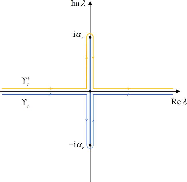
a bijection between ${\chi }_{r}\in {\mathbb{R}}$ and points λ on either contour ${{\rm{\Upsilon }}}_{r}^{+}$ or ${{\rm{\Upsilon }}}_{r}^{-}$ is established by the local polar coordinate system. The oriented contours ${{\rm{\Upsilon }}}_{r}^{\pm }$ are depicted in figure 1.
Figure 1. Geometric illustration of the oriented contours ${{\rm{\Upsilon }}}_{r}^{\pm }$.
An application of the Jordan's lemma, in conjunction with Fourier inverse transformation of the δ function, yields the integral identity:
$\begin{eqnarray*}\frac{1}{2\pi }{\int }_{-\infty }^{+\infty }\left(\begin{array}{c}\frac{\mathop{-{\rm{i}}{u}_{r}^{* }}\limits^{1}}{\lambda +{\chi }_{r}}\end{array}\right){{\rm{e}}}^{{\rm{i}}{\chi }_{r}(\eta -\zeta )}\,{\rm{d}}{\chi }_{r}=\left(\begin{array}{c}\delta (\eta -\zeta )\\ 0\end{array}\right).\end{eqnarray*}$
Subsequent formal integration of equation (3.7) with respect to χr, combined with this result, leads to
$\begin{eqnarray}\begin{array}{l}J=A\left(x+\eta \right)+{\boldsymbol{F}}\left(x,\eta \right)\left(\begin{array}{c}1\\ 0\end{array}\right)\\ \,+{\displaystyle \int }_{x}^{+\infty }{\boldsymbol{F}}\left(x,\zeta \right)A\left(\eta +\zeta \right){\rm{d}}\zeta ,\end{array}\end{eqnarray}$
where
$\begin{eqnarray}\begin{array}{l}J=\frac{1}{2\pi }{\displaystyle \int }_{-\infty }^{+\infty }\left(\frac{q\left(x,\lambda \right){{\rm{e}}}^{{\rm{i}}{\chi }_{r}x}}{{s}_{11}\left(\lambda \right)}-{{\boldsymbol{\varpi }}}_{r,1}\left(\lambda \right)\right){{\rm{e}}}^{{\rm{i}}{\chi }_{r}\left(\eta -x\right)}{\rm{d}}{\chi }_{r},\\ A\left(y\right)=\frac{1}{2\pi }{\displaystyle \int }_{-\infty }^{+\infty }{\beta }_{r}\left(\lambda \right){{\boldsymbol{\varpi }}}_{r,2}\left(\lambda \right){{\rm{e}}}^{{\rm{i}}{\chi }_{r}y}{\rm{d}}{\chi }_{r}.\end{array}\end{eqnarray}$
As stated in equation (3.8), $\lambda =\lambda \left({\chi }_{r}\right)$ and $\lambda \in {{\rm{\Upsilon }}}_{r}^{+}$ in these integral equations. Similar to the results in [40], using Cauchy's residue theorem and Jordan's lemma one can derive an expression for J, which generates
$\begin{eqnarray}\begin{array}{l}{A}_{r}\left(\eta +x\right)+{\boldsymbol{F}}\left(x,\eta \right)\left(\begin{array}{c}1\\ 0\end{array}\right)\\ \,+{\displaystyle \int }_{x}^{+\infty }{\boldsymbol{F}}\left(x,\zeta \right){A}_{r}\left(\eta +\zeta \right){\rm{d}}\zeta =\left(\begin{array}{c}0\\ 0\end{array}\right),\end{array}\end{eqnarray}$
with
$\begin{eqnarray}\begin{array}{l}{A}_{r}\left(y\right)=A\left(y\right)-\hat{A}\left(y\right),\\ \hat{A}\left(y\right)={\rm{i}}\displaystyle \sum _{k=1}^{K}{C}_{k}{{\boldsymbol{\varpi }}}_{r,2}\left({\lambda }_{k}\right){{\rm{e}}}^{{\rm{i}}{\chi }_{r}\left({\lambda }_{k}\right)y}.\end{array}\end{eqnarray}$
For x < η, multiplying the equation (3.5) by ${{\rm{e}}}^{-{\rm{i}}{\chi }_{r}\eta }$ and substituting it into equation (3.1), and subsequently using the same method as before, we get
$\begin{eqnarray}\begin{array}{l}{\tilde{A}}_{r}\left(\eta +x\right){\boldsymbol{F}}\left(x,\eta \right)\left(\begin{array}{c}0\\ 1\end{array}\right)\\ +{\displaystyle \int }_{x}^{+\infty }{\boldsymbol{F}}\left(x,\zeta \right){\tilde{A}}_{r}\left(\zeta +\eta \right){\rm{d}}\zeta =\left(\begin{array}{c}0\\ 0\end{array}\right),\end{array}\end{eqnarray}$
where
$\begin{eqnarray}{\tilde{A}}_{r}\left(y\right)=\tilde{A}\left(y\right)-\tilde{\hat{A}}\left(y\right),\end{eqnarray}$
with
$\begin{eqnarray*}\begin{array}{l}\tilde{A}\left(y\right)=\frac{1}{2\pi }{\displaystyle \int }_{-\infty }^{+\infty }{\tilde{\beta }}_{r}\left(\lambda \right){{\boldsymbol{\varpi }}}_{r,1}\left(\lambda \right){{\rm{e}}}^{-{\rm{i}}{\chi }_{r}y}{\rm{d}}{\chi }_{r},\\ \tilde{\hat{A}}\left(y\right)=-{\rm{i}}\displaystyle \sum _{k=1}^{K}{\tilde{C}}_{k}{{\boldsymbol{\varpi }}}_{r,1}\left({\lambda }_{k}^{* }\right){{\rm{e}}}^{-{\rm{i}}{\chi }_{r}\left({\lambda }_{k}^{* }\right)y}.\end{array}\end{eqnarray*}$
In the above integral equations $\lambda =\lambda ({\chi }_{r})\in {{\rm{\Upsilon }}}_{r}^{-}$ as illustrated in figure 1. It follows from the symmetries of the scattering coefficients and eigenfunctions that the quantities satisfy the relations
$\begin{eqnarray*}\begin{array}{l}{A}^{* }\left(y\right)={\rm{i}}{{\boldsymbol{\sigma }}}_{2}\tilde{A}\left(y\right),{\hat{A}}^{* }\left(y\right)={\rm{i}}{{\boldsymbol{\sigma }}}_{2}\tilde{\hat{A}}\left(y\right),\\ {A}_{r}^{* }\left(y\right)={\rm{i}}{{\boldsymbol{\sigma }}}_{2}{\tilde{A}}_{r}\left(y\right).\end{array}\end{eqnarray*}$
A combination of equations (3.11) and (3.13) leads to the 2 × 2 matrix Marchenko integral equation
$\begin{eqnarray*}{{\boldsymbol{A}}}_{r}\left(x+\eta \right)+{\boldsymbol{F}}\left(x,\eta \right)+{\int }_{x}^{+\infty }{\boldsymbol{F}}\left(x,\zeta \right){{\boldsymbol{A}}}_{r}\left(\eta +\zeta \right){\rm{d}}\zeta ={\bf{0}},\end{eqnarray*}$
where ${{\boldsymbol{A}}}_{r}\left(y\right)=\left({A}_{r}\left(y\right),{\tilde{A}}_{r}\left(y\right)\right)$. Finally, the following properties of ${{\boldsymbol{A}}}_{r}\left(y\right)$ can be readily verified
$\begin{eqnarray*}{{\boldsymbol{A}}}_{r}\left(y\right)=-{{\boldsymbol{\sigma }}}_{3}{{\boldsymbol{A}}}_{r}\left(y\right){{\boldsymbol{\sigma }}}_{3},{{\boldsymbol{A}}}_{r}^{* }\left(y\right)={{\boldsymbol{\sigma }}}_{2}{{\boldsymbol{A}}}_{r}\left(y\right){{\boldsymbol{\sigma }}}_{2}.\end{eqnarray*}$

3.2.2. Left Marchenko integral equation

The second relation in equation (2.16) takes the explicit form
$\begin{eqnarray}\frac{\tilde{p}\left(x,\lambda \right)}{{\tilde{s}}_{11}\left(\lambda \right)}={\tilde{\beta }}_{l}\left(\lambda \right)\tilde{q}\left(x,\lambda \right)+q\left(x,\lambda \right),\lambda \in {\mathbb{R}},\end{eqnarray}$
$\begin{eqnarray}\frac{p\left(x,\lambda \right)}{{\tilde{s}}_{22}\left(\lambda \right)}={\beta }_{l}\left(\lambda \right)q\left(x,\lambda \right)+\tilde{q}\left(x,\lambda \right),\lambda \in {\mathbb{R}}.\end{eqnarray}$
We multiply equation (3.15) by e−iλη for η < x and substitute it into the expression (3.2). By formally integrating over $\lambda \in {\mathbb{R}}$, we obtain
$\begin{eqnarray}\begin{array}{l}\tilde{J}=B\left(\eta +x\right)+{\boldsymbol{G}}\left(x,\eta \right)\left(\begin{array}{c}0\\ 1\end{array}\right)\\ +{\displaystyle \int }_{-\infty }^{x}{\boldsymbol{G}}\left(x,\zeta \right)B\left(\eta +\zeta \right){\rm{d}}\zeta ,\end{array}\end{eqnarray}$
where
$\begin{eqnarray*}\begin{array}{l}\tilde{J}=\frac{1}{2\pi }{\displaystyle \int }_{-\infty }^{+\infty }\left[\frac{p\left(x,\lambda \right){{\rm{e}}}^{-{\rm{i}}\lambda x}}{\tilde{{s}_{22}}\left(\lambda \right)}-\left(\begin{array}{c}0\\ 1\end{array}\right)\right]{{\rm{e}}}^{{\rm{i}}\lambda \left(x-\eta \right)}{\rm{d}}\lambda ,\\ B\left(y\right)=\frac{1}{2\pi }{\displaystyle \int }_{-\infty }^{+\infty }{\beta }_{l}\left(\lambda \right){{\rm{e}}}^{-{\rm{i}}\lambda y}\left(\begin{array}{c}1\\ 0\end{array}\right){\rm{d}}\lambda .\end{array}\end{eqnarray*}$
Our next objective is to express $\tilde{J}$ in terms of the Marchenko kernel ${\boldsymbol{G}}\left(x,\zeta \right)$. This requires a closed path in the upper half of the λ-plane to encircle the contribution from ${{\rm{\Theta }}}_{r}^{+}$. Accordingly, we define a closed contour ${\rm{\Upsilon }}\left({R}_{\infty },{R}_{\varepsilon }\right)$, with 0 < Rϵ < R < +, as comprising the following six segments: (1) the real-segment $\left[-{R}_{\infty },-{R}_{\varepsilon }\right]$; (2) the imaginary-axis segment $\left[-{R}_{\varepsilon }+{\rm{i}}0,-{R}_{\varepsilon }+{\rm{i}}{\alpha }_{r}\right]$; (3) the semicircle $\left\{{\rm{i}}{\alpha }_{r}+{R}_{\varepsilon }{{\rm{e}}}^{{\rm{i}}\left[\pi -\theta \right]}:0\leqslant \theta \lt \pi \right\}$ with clockwise direction; (4) the imaginary-axis segment $\left[{R}_{\varepsilon }+{\rm{i}}0,{R}_{\varepsilon }+{\rm{i}}{\alpha }_{r}\right]$; (5) the real-axis segment $\left[{R}_{\varepsilon },{R}_{\infty }\right]$; (6) the large semicircle $\left\{{R}_{\infty }{{\rm{e}}}^{{\rm{i}}\theta }:0\leqslant \theta \lt \pi \right\}$ with counterclockwise direction.
We identify two nontrivial contributions to the integral in equation (3.17), such that $\tilde{J}={\tilde{J}}_{1}+{\tilde{J}}_{2}$. Here, ${\tilde{J}}_{1}$ corresponds to the residue at ${\lambda }_{k}\in {{\mathbb{D}}}_{r}^{+}$, and ${\tilde{J}}_{2}$ comes from the contour integral along $\lambda \in {{\rm{\Theta }}}_{r}^{+}$. These two contributions are discussed in detail in the following.
Under the assumption that the ${\lambda }_{k}\in {{\mathbb{D}}}_{r}^{+}$ are zeros of ${\tilde{s}}_{22}\left(\lambda \right)$, and observing the continuity of $1/{\tilde{s}}_{22}\left(\lambda \right)$ and the transmission coefficient, the relation $p\left(x,{\lambda }_{k}\right)=q\left(x,{\lambda }_{k}\right)/{c}_{k}$ yields
$\begin{eqnarray*}{\tilde{J}}_{1}={\rm{i}}\displaystyle \sum _{k=1}^{K}{\tilde{C}}_{k}q\left(x,{\lambda }_{k}\right){{\rm{e}}}^{-{\rm{i}}{\lambda }_{k}\eta },\end{eqnarray*}$
where ${\tilde{C}}_{k}={\tilde{\xi }}_{k}/{c}_{k}$, and ${\tilde{\xi }}_{k}$ represents the residue of ${\tilde{s}}_{22}^{-1}\left(\lambda \right)$ at λ = λk. Thus, we obtain
$\begin{eqnarray*}{\tilde{J}}_{1}={B}_{1}\left(x+\eta \right)+{\int }_{-\infty }^{x}{\boldsymbol{G}}\left(x,\zeta \right){B}_{1}\left(\eta +\zeta \right){\rm{d}}\zeta ,\end{eqnarray*}$
$\begin{eqnarray*}{B}_{1}\left(y\right)={\rm{i}}\displaystyle \sum _{k=1}^{K}{\tilde{C}}_{k}{{\rm{e}}}^{-{\rm{i}}{\lambda }_{k}x}\left(\begin{array}{c}1\\ 0\end{array}\right).\end{eqnarray*}$
Furthermore, the following relationships for the residues ${\tilde{\xi }}_{k}$, ξk and the norming constants ${\tilde{C}}_{k}$, Ck can be deduced from the expressions of the scattering coefficients
$\begin{eqnarray}{\tilde{\xi }}_{k}={\xi }_{k}\frac{{\lambda }_{k}+{\chi }_{r}\left({\lambda }_{k}\right)}{2{\chi }_{r}\left({\lambda }_{k}\right)},\tilde{{C}_{k}}{C}_{k}={\xi }_{k}^{2}\frac{{\lambda }_{k}+{\chi }_{r}\left({\lambda }_{k}\right)}{2{\chi }_{r}\left({\lambda }_{k}\right)}.\end{eqnarray}$
We now turn to ${\tilde{J}}_{2}$, which originates from the integral along $\lambda \in {{\rm{\Theta }}}_{r}^{+}$ with ${\chi }_{r}\in {\mathbb{R}}$. Direct computation yields
$\begin{eqnarray*}\begin{array}{l}{\tilde{J}}_{2}=\mathop{\mathrm{lim}}\limits_{\varepsilon \to 0}\frac{1}{2\pi }\left({\displaystyle \int }_{{\rm{i}}0-\varepsilon }^{{\rm{i}}{\alpha }_{r}-\varepsilon }\left[\frac{p\left(x,\lambda \right)}{{\tilde{s}}_{22}\left(\lambda \right)}{{\rm{e}}}^{-{\rm{i}}\lambda x}-\left(\begin{array}{c}0\\ 1\end{array}\right)\right]{{\rm{e}}}^{{\rm{i}}\lambda \left(x-\eta \right)}{\rm{d}}\lambda \right)\\ -\mathop{\mathrm{lim}}\limits_{\varepsilon \to 0}\frac{1}{2\pi }\left({\displaystyle \int }_{{\rm{i}}0+\varepsilon }^{{\rm{i}}{\alpha }_{r}+\varepsilon }\left[\frac{p\left(x,\lambda \right)}{{\tilde{s}}_{22}\left(\lambda \right)}{{\rm{e}}}^{-{\rm{i}}\lambda x}-\left(\begin{array}{c}0\\ 1\end{array}\right)\right]{{\rm{e}}}^{{\rm{i}}\lambda \left(x-\eta \right)}{\rm{d}}\lambda \right)\\ =\frac{1}{2\pi }{\displaystyle \int }_{0}^{{\rm{i}}{\alpha }_{r}}\left[\frac{{p}^{-}\left(x,\lambda \right)}{{\tilde{s}}_{22}^{-}\left(\lambda \right)}-\frac{{p}^{+}\left(x,\lambda \right)}{{\tilde{s}}_{22}^{+}\left(\lambda \right)}\right]{{\rm{e}}}^{-{\rm{i}}\lambda \eta }{\rm{d}}\lambda .\end{array}\end{eqnarray*}$
For integrals along ${{\rm{\Theta }}}_{r}^{+}$, the notation ± indicates the right/left limiting values on the branch cut. Taking the scattering coefficients in equation (2.20) into account, the above equation becomes
$\begin{eqnarray}\begin{array}{rcl}{\tilde{J}}_{2} & = & -\frac{1}{2\pi }{\displaystyle \int }_{0}^{{\rm{i}}{\alpha }_{r}}\left[\frac{\lambda -{\chi }_{r}^{+}(\lambda )}{2{\chi }_{r}^{+}(\lambda )}\frac{{p}^{-}\left(x,\lambda \right)}{{s}_{11}^{-}\left(\lambda \right)}\right.\\ & & \left.+\frac{\lambda +{\chi }_{r}^{+}(\lambda )}{2{\chi }_{r}^{+}(\lambda )}\frac{{p}^{+}\left(x,\lambda \right)}{{s}_{11}^{+}\left(\lambda \right)}\right]{{\rm{e}}}^{-{\rm{i}}\lambda \eta }{\rm{d}}\lambda .\end{array}\end{eqnarray}$
The symmetries (2.24) and (2.25) allow to express $({\chi }_{r}^{+}(\lambda )-\lambda ){p}^{-}/{s}_{11}=-({\chi }_{r}^{+}(\lambda )+\lambda ){p}^{+}/{s}_{21}$, which makes the integral equation (3.19) simplify to
$\begin{eqnarray*}\begin{array}{l}{\tilde{J}}_{2}=-\frac{1}{4\pi }{\displaystyle \int }_{0}^{{\rm{i}}{\alpha }_{r}}\frac{{\chi }_{r}^{+}(\lambda )+\lambda }{{\chi }_{r}^{+}(\lambda )}\left[\frac{{\tilde{p}}^{+}\left(x,\lambda \right)}{{s}_{21}^{+}\left(\lambda \right)}+\frac{{p}^{+}\left(x,\lambda \right)}{{s}_{11}^{+}\left(\lambda \right)}\right]{{\rm{e}}}^{-{\rm{i}}\lambda \eta }{\rm{d}}\lambda .\end{array}\end{eqnarray*}$
With the help of scattering equation (3.3), we get
$\begin{eqnarray*}\begin{array}{l}{\tilde{J}}_{2}=-\frac{1}{4\pi }{\displaystyle \int }_{0}^{{\rm{i}}{\alpha }_{r}}\frac{{\chi }_{r}^{+}(\lambda )+\lambda }{{\chi }_{r}^{+}(\lambda )}\frac{{q}^{+}\left(x,\lambda \right)}{{s}_{11}^{+}\left(\lambda \right){s}_{21}^{+}\left(\lambda \right)}{{\rm{e}}}^{-{\rm{i}}\lambda \eta }{\rm{d}}\lambda \\ =\frac{{\rm{i}}{u}_{r}}{4\pi }{\displaystyle \int }_{0}^{{\rm{i}}{\alpha }_{r}}\frac{1}{{\chi }_{r}^{+}(\lambda )}\frac{{q}^{+}\left(x,\lambda \right)}{{s}_{11}^{-}\left(\lambda \right){s}_{11}^{+}\left(\lambda \right)}{{\rm{e}}}^{-{\rm{i}}\lambda \eta }{\rm{d}}\lambda .\end{array}\end{eqnarray*}$
Using the triangular expression (3.2) yields
$\begin{eqnarray}\begin{array}{l}{\tilde{J}}_{2}={A}_{2}\left(x+\eta \right)+{\displaystyle \int }_{-\infty }^{x}{\boldsymbol{G}}\left(x,\zeta \right){B}_{2}\left(\eta +\zeta \right){\rm{d}}\zeta ,\end{array}\end{eqnarray}$
where
$\begin{eqnarray*}{B}_{2}\left(y\right)=\frac{{\rm{i}}{u}_{r}}{4\pi }{\int }_{0}^{{\rm{i}}{\alpha }_{r}}\frac{1}{{\chi }_{r}^{+}(\lambda )}\frac{1}{{s}_{11}^{-}\left(\lambda \right){s}_{11}^{+}\left(\lambda \right)}\left(\begin{array}{c}1\\ 0\end{array}\right){{\rm{e}}}^{-{\rm{i}}\lambda y}{\rm{d}}\lambda .\end{eqnarray*}$
Combining equations (3.18) and (3.20), and substituting the result into equation (3.17), leads to the expression
$\begin{eqnarray}\begin{array}{rc} & {B}_{l}\left(\eta +x\right)+{\boldsymbol{G}}\left(x,\eta \right)\left(\begin{array}{c}0\\ 1\end{array}\right)\\ & +{\displaystyle \int }_{-\infty }^{x}{\boldsymbol{G}}\left(x,\zeta \right){B}_{l}\left(\eta +\zeta \right){\rm{d}}\zeta =\left(\begin{array}{c}0\\ 0\end{array}\right),\end{array}\end{eqnarray}$
where ${B}_{l}\left(y\right)=B\left(y\right)-{B}_{1}\left(y\right)-{B}_{2}\left(y\right)$.
Beginning with equation (3.16), a similar procedure leads to the result
$\begin{eqnarray}\begin{array}{rc} & {\tilde{B}}_{l}\left(\eta +x\right)+{\boldsymbol{G}}\left(x,\eta \right)\left(\begin{array}{c}1\\ 0\end{array}\right)\\ & +{\displaystyle \int }_{-\infty }^{x}{\boldsymbol{G}}\left(x,\zeta \right){\tilde{B}}_{l}\left(\zeta +\eta \right){\rm{d}}\zeta =\left(\begin{array}{c}0\\ 0\end{array}\right),\end{array}\end{eqnarray}$
where ${\tilde{B}}_{l}\left(y\right)={\rm{i}}{{\boldsymbol{\sigma }}}_{2}{B}_{l}^{* }\left(y\right)$. The Marchenko integral equation is formed by combining equations (3.21) and (3.22), expressed as
$\begin{eqnarray*}{{\boldsymbol{B}}}_{l}\left(\eta +x\right)+{\boldsymbol{G}}\left(x,\eta \right)+{\int }_{-\infty }^{x}{\boldsymbol{G}}\left(x,\zeta \right){{\boldsymbol{B}}}_{l}\left(\eta +\zeta \right){\rm{d}}\zeta ={\bf{0}},\end{eqnarray*}$
where ${{\boldsymbol{B}}}_{l}\left(y\right)=\left(\tilde{{B}_{l}}\left(\lambda \right),{B}_{l}\left(\lambda \right)\right)$ and ${{\boldsymbol{B}}}_{l}^{* }\left(y\right)={{\boldsymbol{\sigma }}}_{2}{{\boldsymbol{B}}}_{l}\left(y\right){{\boldsymbol{\sigma }}}_{2}.$
The above results show that the one-sided NZBC with αr > 0 gives rise to the asymmetry between the right and left Marchenko integral equations. If the boundary condition becomes u(tx) → 0 as x → +, and $u(t,x)\,\to {u}_{l}(t)={\alpha }_{l}{{\rm{e}}}^{2{\rm{i}}{\gamma }_{1}{\alpha }_{l}^{2}t+{\rm{i}}{\nu }_{l}}$ as x → −, with 0 ≤ νl < 2π, αl > 0 are arbitrary constants, then the roles of the two Marchenko integral equations above would be interchanged.

Note that in equation (3.11), βr(λ) is integrated for all ${\chi }_{r}\in {\mathbb{R}}$, which indicates that the integral contains the contribution of λ ∈ Θr besides the continuous spectrum $\lambda \in {\mathbb{R}}$. Furthermore, the existence of symmetries (2.28) leads to the fact that the integrals over Θr can never be set identically to zero, which means that when ${{\rm{\Theta }}}_{r}\ne {\rm{\varnothing }}$ (corresponding to the one-sided NZBC (1.2) with αr > 0), pure soliton solutions do not exist.

3.3. Riemann–Hilbert problem

The goal of the present section is to construct appropriate right and left matrix RH problems using sectionally meromorphic functions in the cut plane ${{\mathbb{D}}}_{r}$, which are used to express the inverse problem.

3.3.1. Right Riemann–Hilbert problem

According to the analytic properties as well as asymptotic behavior of the scattering coefficients and Jost solutions, we introduce the following sectionally meromorphic matrix
$\begin{eqnarray*}{\boldsymbol{M}}\left(x,\lambda \right)=\left\{\begin{array}{ll}\left[\frac{q\left(x,\lambda \right)}{{s}_{11}\left(\lambda \right)}{{\rm{e}}}^{{\rm{i}}\lambda x},p\left(x,\lambda \right){{\rm{e}}}^{-{\rm{i}}{\chi }_{r}x}\right],\quad & \lambda \in {{\mathbb{D}}}_{r}^{+},\\ \left[\tilde{p}\left(x,\lambda \right){{\rm{e}}}^{{\rm{i}}{\chi }_{r}x},\frac{\tilde{q}\left(x,\lambda \right)}{{s}_{22}\left(\lambda \right)}{{\rm{e}}}^{-{\rm{i}}\lambda x}\right],\quad & \lambda \in {{\mathbb{D}}}_{r}^{-},\end{array}\right.\end{eqnarray*}$
and ${\boldsymbol{M}}\left(x,\lambda \right)\to {\boldsymbol{I}}$ as $\left|\lambda \right|\to \infty $. Clearly, we have three jump matrices: V1 denotes the jump matrix across real axis ${\mathbb{R}}$, V2 and V3 are associated with the jumps across ${{\rm{\Theta }}}_{r}^{+}$ and ${{\rm{\Theta }}}_{r}^{-}$, respectively. These three jump matrices have dependence on the spectral parameter λ along their specified contour and are parametrically dependent on $(x,t)\in {\mathbb{R}}\times {{\mathbb{R}}}^{+}$. Moreover, the dependence on x is expressed directly, while the time dependence is reflected in the time evolution of the scattering data.
Across the real axis ${\mathbb{R}}$, the jump condition for the RH problem is given by the matrix relation ${{\boldsymbol{M}}}^{+}\left(x,\lambda \right)\,={{\boldsymbol{M}}}^{-}\left(x,\lambda \right){{\boldsymbol{V}}}_{1}\left(x,\lambda \right)$, with the corresponding explicit expression
$\begin{eqnarray*}\begin{array}{l}\left(\frac{{q}^{+}\left(x,\lambda \right)}{{s}_{11}^{+}\left(\lambda \right)}{{\rm{e}}}^{{\rm{i}}\lambda x},{p}^{+}\left(x,\lambda \right){{\rm{e}}}^{-{\rm{i}}{\chi }_{r}x}\right)\\ \quad =\left({\tilde{p}}^{-}\left(x,\lambda \right){{\rm{e}}}^{{\rm{i}}{\chi }_{r}x},\frac{{\tilde{q}}^{-}\left(x,\lambda \right)}{{s}_{22}^{-}\left(\lambda \right)}{{\rm{e}}}^{-{\rm{i}}\lambda x}\right){{\boldsymbol{V}}}_{1}\left(x,\lambda \right),\lambda \in {\mathbb{R}}.\end{array}\end{eqnarray*}$
In this scenario, ± denote the limiting values from the upper/lower λ-plane, and ${{\boldsymbol{V}}}_{1}\left(x,\lambda \right)$ can be explicitly derived from the scattering matrix S(λ) through direct computation as
$\begin{eqnarray*}{{\boldsymbol{V}}}_{1}\left(x,\lambda \right)=\left(\begin{array}{cc}\left[1-{\beta }_{r}\left(\lambda \right){\tilde{\beta }}_{r}\left(\lambda \right)\right]{{\rm{e}}}^{{\rm{i}}\left(\lambda -{\chi }_{r}\right)x} & -{\tilde{\beta }}_{r}\left(\lambda \right){{\rm{e}}}^{-2{\rm{i}}{\chi }_{r}x}\\ {\beta }_{r}\left(\lambda \right){{\rm{e}}}^{2{\rm{i}}\lambda x} & {{\rm{e}}}^{{\rm{i}}\left(\lambda -{\chi }_{r}\right)x}\end{array}\right).\end{eqnarray*}$
Subsequently, the RH problem across ${{\rm{\Theta }}}_{r}^{+}$ is denoted by ${{\boldsymbol{M}}}^{+}\left(x,\lambda \right)={{\boldsymbol{M}}}^{-}\left(x,\lambda \right){{\boldsymbol{V}}}_{2}\left(x,\lambda \right)$, with the superscript ± denoting the boundary values originating from the right and left sides of ${{\rm{\Theta }}}_{r}^{+}$, respectively. Based on equation (2.12) and noting that for $\lambda \in {{\rm{\Theta }}}_{r}^{+}$, q+(xλ) = q(xλ), we get
$\begin{eqnarray}\begin{array}{l}\left(\frac{{q}^{+}\left(x,\lambda \right)}{{s}_{11}^{+}\left(\lambda \right)}{{\rm{e}}}^{{\rm{i}}\lambda x},{p}^{+}\left(x,\lambda \right){{\rm{e}}}^{-{\rm{i}}{\chi }_{r}^{+}x}\right)\\ \quad =\left(\frac{{q}^{-}\left(x,\lambda \right)}{{s}_{11}^{-}\left(\lambda \right)}{{\rm{e}}}^{{\rm{i}}\lambda x},{p}^{-}\left(x,\lambda \right){{\rm{e}}}^{-{\rm{i}}{\chi }_{r}^{-}x}\right)\\ \times {{\boldsymbol{V}}}_{2}\left(x,\lambda \right),\lambda \in {{\mathbb{C}}}^{+}.\end{array}\end{eqnarray}$
The definition (2.16) of S(λ) yields
$\begin{eqnarray*}{q}^{\pm }(x,\lambda )={s}_{11}^{\pm }(\lambda ){\tilde{p}}^{\pm }(x,\lambda )+{s}_{21}^{\pm }(\lambda ){p}^{\pm }(x,\lambda ),\lambda \in {{\rm{\Theta }}}_{r}^{+},\end{eqnarray*}$
and leveraging the symmetry relations (2.26) gives
$\begin{eqnarray}\begin{array}{l}\frac{{q}^{+}(x,\lambda )}{{s}_{11}^{+}(\lambda )}=-\frac{{\rm{i}}{u}_{r}^{* }}{{\chi }_{r}^{+}(\lambda )+\lambda }{p}^{-}(x,\lambda )\\ +{\beta }_{r}^{+}(\lambda ){p}^{+}(x,\lambda ),\end{array}\end{eqnarray}$
$\begin{eqnarray}\begin{array}{l}{p}^{+}(x,\lambda )=-\frac{{\rm{i}}{u}_{r}}{{\chi }_{r}^{+}(\lambda )+\lambda }\\ \,\times \,\left[\frac{{q}^{-}(x,\lambda )}{{s}_{11}^{-}(\lambda )}-{\beta }_{r}^{-}(\lambda ){p}^{-}(x,\lambda )\right].\end{array}\end{eqnarray}$
Bringing equation (3.25) into (3.24) yields
$\begin{eqnarray}\begin{array}{l}\frac{{q}^{+}(x,\lambda )}{{s}_{11}^{+}(\lambda )}=-\frac{{\rm{i}}{u}_{r}}{{\chi }_{r}^{+}(\lambda )+\lambda }\\ \,\times \,\left[\frac{{q}^{-}(x,\lambda )}{{s}_{11}^{-}(\lambda )}{\beta }_{r}^{-}(\lambda )+\left(\frac{{u}_{r}^{* }}{{u}_{r}}-{\beta }_{r}^{+}(\lambda ){\beta }_{r}^{-}(\lambda )\right){p}^{-}(x,\lambda )\right].\end{array}\end{eqnarray}$
Using equations (3.25), (3.26) and (3.23) as well as noting that equation (2.27), one can derive ${{\boldsymbol{V}}}_{2}\left(x,\lambda \right)$ as
$\begin{eqnarray*}{{\boldsymbol{V}}}_{2}\left(x,\lambda \right)=-\frac{{\rm{i}}{u}_{r}}{\lambda +{\chi }_{r}^{+}(\lambda )}\left(\begin{array}{cc}{\beta }_{r}^{+}\left(\lambda \right) & {{\rm{e}}}^{-{\rm{i}}\left({\chi }_{r}^{+}(\lambda )+\lambda \right)x}\\ 0 & -{\beta }_{r}^{-}\left(\lambda \right){{\rm{e}}}^{-2{\rm{i}}{\chi }_{r}^{+}(\lambda )x}\end{array}\right).\end{eqnarray*}$
Across the contour ${{\rm{\Theta }}}_{r}^{-}$, the RH problem is defined by the relation ${{\boldsymbol{M}}}^{+}\left(x,\lambda \right)={{\boldsymbol{M}}}^{-}\left(x,\lambda \right){{\boldsymbol{V}}}_{3}\left(x,\lambda \right)$, where ± represent the limiting values emanating from the right or left sides of ${{\rm{\Theta }}}_{r}^{-}$. Considering the equation (2.12) and for $\lambda \in {{\rm{\Theta }}}_{r}^{-}$, ${\tilde{q}}^{+}(x,\lambda )={\tilde{q}}^{-}(x,\lambda )$, we get
$\begin{eqnarray}\begin{array}{l}\left({\tilde{p}}^{+}\left(x,\lambda \right){{\rm{e}}}^{{\rm{i}}{\chi }_{r}^{+}x},\frac{{\tilde{q}}^{+}\left(x,\lambda \right)}{{s}_{22}^{+}\left(\lambda \right)}{{\rm{e}}}^{-{\rm{i}}\lambda x}\right)\\ \,\,=\,\left({\tilde{p}}^{-}\left(x,\lambda \right){{\rm{e}}}^{{\rm{i}}{\chi }_{r}^{-}x},\frac{{\tilde{q}}^{-}\left(x,\lambda \right)}{{s}_{22}^{-}\left(\lambda \right)}{{\rm{e}}}^{-{\rm{i}}\lambda x}\right){{\boldsymbol{V}}}_{3}\left(x,\lambda \right),\\ \,\lambda \in {{\mathbb{C}}}^{-}.\end{array}\end{eqnarray}$
To calculate the jump matrix ${{\boldsymbol{V}}}_{3}\left(x,\lambda \right)$ for $\lambda \in {{\mathbb{C}}}^{-}$, we again use the definition (2.16) of the scattering matrix S(λ) to obtain
$\begin{eqnarray*}\frac{{\tilde{q}}^{\pm }(x,\lambda )}{{s}_{22}^{\pm }(\lambda )}={p}^{\pm }(x,\lambda )+{\tilde{\beta }}_{r}^{\pm }(\lambda ){\tilde{p}}^{\pm }(x,\lambda ),\lambda \in {{\rm{\Theta }}}_{r}^{-},\end{eqnarray*}$
and then use the symmetry relations (2.26) to yield
$\begin{eqnarray}\frac{{\tilde{q}}^{+}(x,\lambda )}{{s}_{22}^{+}(\lambda )}={\tilde{\beta }}^{+}(\lambda ){\tilde{p}}^{+}(x,\lambda )-\frac{{\rm{i}}{u}_{r}}{{\chi }_{r}^{+}(\lambda )+\lambda }{\tilde{p}}^{-}(x,\lambda ),\end{eqnarray}$
$\begin{eqnarray}{\tilde{p}}^{+}(x,\lambda )=-\frac{{\rm{i}}{u}_{r}^{* }}{{\chi }_{r}^{+}(\lambda )+\lambda }\left[\frac{{\tilde{q}}^{-}(x,\lambda )}{{s}_{22}^{-}(\lambda )}-{\tilde{\beta }}^{-}(\lambda ){\tilde{p}}^{-}(x,\lambda )\right].\end{eqnarray}$
Bringing equation (3.29) into (3.28), we get
$\begin{eqnarray}\begin{array}{l}\frac{{\tilde{q}}^{+}(x,\lambda )}{{s}_{22}^{+}(\lambda )}=-\frac{{\rm{i}}{u}_{r}^{* }}{{\chi }_{r}^{+}(\lambda )+\lambda }\\ \times \,\left[\frac{{\tilde{q}}^{-}(x,\lambda )}{{s}_{22}^{-}(\lambda )}{\tilde{\beta }}^{+}(\lambda )+\left(\frac{{u}_{r}}{{u}_{r}^{* }}-{\tilde{\beta }}_{r}^{+}(\lambda ){\tilde{\beta }}_{r}^{-}(\lambda )\right){\tilde{p}}^{-}(x,\lambda )\right].\end{array}\end{eqnarray}$
Utilizing equations (3.29), (3.30) and (3.27) as well as noting equation (2.27), the jump matrix ${{\boldsymbol{V}}}_{3}\left(x,\lambda \right)$ is computed to be
$\begin{eqnarray*}{{\boldsymbol{V}}}_{3}\left(x,\lambda \right)=-\frac{{\rm{i}}{u}_{r}^{* }}{\lambda +{\chi }_{r}^{+}(\lambda )}\left(\begin{array}{cc}-{\tilde{\beta }}_{r}^{-}\left(\lambda \right){{\rm{e}}}^{2{\rm{i}}{\chi }_{r}^{+}(\lambda )x} & 0\\ {{\rm{e}}}^{{\rm{i}}\left({\chi }_{r}^{+}(\lambda )+\lambda \right)x} & {\tilde{\beta }}_{r}^{+}\left(\lambda \right)\end{array}\right).\end{eqnarray*}$
And V1(xλ), V2(xλ) satisfy the symmetry relations in the upper/lower half λ-plane, given by
$\begin{eqnarray*}{{\boldsymbol{V}}}_{2}(x,\lambda )={{\boldsymbol{\sigma }}}_{2}{{\boldsymbol{V}}}_{1}^{* }(x,{\lambda }^{* }){{\boldsymbol{\sigma }}}_{2}.\end{eqnarray*}$
Formulating the inverse problem as a RH problem with poles (these correspond to the zeros of the scattering coefficients s11(λ) and s22(λ)) essentially amounts to solving a sectionally meromorphic matrix M(xλ), which is normalized to I as λ →  and satisfies the given jump conditions. On the basis of the above content, we rewrite the problem as ${{\boldsymbol{M}}}^{+}={{\boldsymbol{M}}}^{-}+\left({\boldsymbol{V}}-{\boldsymbol{I}}\right){{\boldsymbol{M}}}^{-}$, where V = Vk(xλ), (k = 1, 2, 3) are contingent upon the specific segment of the oriented contour under consideration. Subsequently, by eliminating the asymptotic behavior as λ →  and the residues of M±(xλ) at the poles in ${{\mathbb{D}}}_{r}^{\pm }$ from both sides, the result is
$\begin{eqnarray}\begin{array}{l}{{\boldsymbol{M}}}^{+}-{\boldsymbol{I}}-\displaystyle \sum _{k=1}^{K}\frac{{{\rm{Res}}}_{{\lambda }_{k}}{{\boldsymbol{M}}}^{+}}{\lambda -{\lambda }_{k}}-\displaystyle \sum _{k=1}^{K}\frac{{{\rm{Res}}}_{{\lambda }_{k}^{* }}{{\boldsymbol{M}}}^{-}}{\lambda -{\lambda }_{k}^{* }}\\ =\,{{\boldsymbol{M}}}^{-}-{\boldsymbol{I}}-\displaystyle \sum _{k=1}^{K}\frac{{{\rm{Res}}}_{{\lambda }_{k}}{{\boldsymbol{M}}}^{+}}{\lambda -{\lambda }_{k}}-\displaystyle \sum _{k=1}^{K}\frac{{{\rm{Res}}}_{{\lambda }_{k}^{* }}{{\boldsymbol{M}}}^{-}}{\lambda -{\lambda }_{k}^{* }}\\ \,+\,\left({\boldsymbol{V}}-{\boldsymbol{I}}\right){{\boldsymbol{M}}}^{-}.\end{array}\end{eqnarray}$
For equation (3.31), the sum of each term on its right-hand side except the last is analytic in ${{\mathbb{D}}}_{r}^{-}$ and O(λ−1) as λ → , while the left hand side is analytic in domain ${{\mathbb{D}}}_{r}^{+}$ and is O(λ−1) as λ → . The projectors Y± on ${{\rm{\Upsilon }}}_{r}^{\pm }={\mathbb{R}}\cup {{\rm{\Theta }}}_{r}^{\pm }$ are defined as
$\begin{eqnarray*}{Y}_{\pm }\left[h\right]\left(k\right)=\frac{1}{2{\rm{i}}\pi }{\int }_{{{\rm{\Upsilon }}}_{r}^{\pm }}\frac{h\left(\zeta \right)}{\zeta -\lambda }{\rm{d}}\zeta ,\end{eqnarray*}$
which are introduced to construct the solution to the RH problem. In the above equation, ${\int }_{{{\rm{\Upsilon }}}_{r}^{\pm }}$ stand for integrals along the oriented contours shown in figure 1, and the limit is taken from the upper/lower when $\lambda \in {\mathbb{R}}\cap {{\rm{\Upsilon }}}_{r}^{\pm }$. We know that if h± are analytic in ${{\mathbb{D}}}_{r}^{\pm }$ and O(λ−1) as λ → , then Yh+ = Y+h = 0 and Y±h± = ± h± hold. By using Y± at both ends of the equation (3.31), we get
$\begin{eqnarray}\begin{array}{l}{\boldsymbol{M}}\left(x,\lambda \right)={\boldsymbol{I}}+\displaystyle \sum _{k=1}^{K}\frac{{{\rm{Res}}}_{{\lambda }_{k}}{{\boldsymbol{M}}}^{+}}{\lambda -{\lambda }_{k}}\\ \,+\,\displaystyle \sum _{k=1}^{K}\frac{{{\rm{Res}}}_{{\lambda }_{k}^{* }}{{\boldsymbol{M}}}^{-}}{\lambda -{\lambda }_{k}^{* }}\\ \,+\,\frac{1}{2{\rm{i}}\pi }{\displaystyle \int }_{{{\rm{\Upsilon }}}_{r}^{\pm }}\frac{{{\boldsymbol{M}}}^{-}\left(\zeta \right)}{\zeta -\lambda }\left[{\boldsymbol{V}}\left(\zeta \right)-{\boldsymbol{I}}\right]{\rm{d}}\zeta .\end{array}\end{eqnarray}$
Based on equations (2.30) and (2.31), the 2nd column of ${{\rm{Res}}}_{{\lambda }_{k}}{{\boldsymbol{M}}}^{+}$ equals zero for all k, whereas the 1st column is a scalar multiple of the 2nd column of M+(xλk). Conversely, the 1st column of ${{\rm{Res}}}_{{\lambda }_{k}^{* }}{{\boldsymbol{M}}}^{-}$ equals zero for all k, whereas the 2nd column is a scalar multiple of the 2nd column of ${{\boldsymbol{M}}}^{-}(x,{\lambda }_{k}^{* })$. The reconstruction formula for the potential function can be deduced from the large λ asymptotic expansion
$\begin{eqnarray*}{{\boldsymbol{M}}}^{(O)}\left(x,\lambda \right)=\frac{{\rm{i}}}{2\lambda }{\boldsymbol{U}}(x){{\boldsymbol{\sigma }}}_{3}+o({\lambda }^{-1}),\end{eqnarray*}$
a result that is formalized in the theorem below.

The potential function admits the following reconstruction formula

$\begin{eqnarray}u\left(x\right)=2{\rm{i}}\mathop{\mathrm{lim}}\limits_{\lambda \to \infty }\lambda {{\boldsymbol{M}}}_{12}\left(x,\lambda \right).\end{eqnarray}$

In the reconstruction formula presented above, the temporal dependence is introduced through the time evolution of the scattering data.

Unlike the symmetric NZBC, the above reconstruction formulation cannot be reduced to a purely algebraic system by employing the reflectionless condition. Even though we can choose the reflection coefficients equal to zero on the continuous spectrum $\lambda \in {\mathbb{R}}$, the integrals of equation (3.32) still have a nonzero contribution due to ${{\rm{\Theta }}}_{r}^{\pm }$. Consequently, no pure soliton solutions exist under the one-sided NZBC.

3.3.2. Left Riemann–Hilbert problem

The left scattering data can also be utilized to construct a proper RH problem and then formulate the inverse problem. Firstly, we introduce the following matrix
$\begin{eqnarray*}\tilde{{\boldsymbol{M}}}\left(x,\lambda \right)=\left\{\begin{array}{l}\left[q\left(x,\lambda \right){{\rm{e}}}^{{\rm{i}}\lambda x},\frac{p\left(x,\lambda \right)}{{\tilde{s}}_{22}\left(\lambda \right)}{{\rm{e}}}^{-{\rm{i}}{\chi }_{r}x}\right],\lambda \in {{\mathbb{D}}}_{r}^{+},\\ \left[\frac{\tilde{p}\left(x,\lambda \right)}{{\tilde{s}}_{11}\left(\lambda \right)}{{\rm{e}}}^{{\rm{i}}{\chi }_{r}x},\tilde{q}\left(x,\lambda \right){{\rm{e}}}^{-{\rm{i}}\lambda x}\right],\lambda \in {{\mathbb{D}}}_{r}^{-}.\end{array}\right.\end{eqnarray*}$
The RH problem across ${\mathbb{R}}$ is formulated in the matrix form ${\tilde{{\boldsymbol{M}}}}^{+}\left(x,\lambda \right)={\tilde{{\boldsymbol{M}}}}^{-}\left(x,\lambda \right){\tilde{{\boldsymbol{V}}}}_{1}\left(x,\lambda \right)$, i.e.
$\begin{eqnarray*}\begin{array}{l}\left({q}^{+}\left(x,\lambda \right){{\rm{e}}}^{{\rm{i}}\lambda x},\frac{{p}^{+}\left(x,\lambda \right)}{{\tilde{{s}_{22}}}^{+}\left(\lambda \right)}{{\rm{e}}}^{-{\rm{i}}{\chi }_{r}x}\right)\\ \,\,\,=\,\left(\frac{{\tilde{p}}^{-}\left(x,\lambda \right)}{{\tilde{{s}_{11}}}^{-}\left(\lambda \right)}{{\rm{e}}}^{{\rm{i}}{\chi }_{r}x},{\tilde{q}}^{-}\left(x,\lambda \right){{\rm{e}}}^{-{\rm{i}}\lambda x}\right){\tilde{{\boldsymbol{V}}}}_{1}\left(x,\lambda \right),\\ \,\,\,\lambda \in {\mathbb{R}},\end{array}\end{eqnarray*}$
where ± represent the limiting values from the upper/lower complex planes, and ${\tilde{{\boldsymbol{V}}}}_{1}\left(x,\lambda \right)$ is obtained from equation (2.16) as
$\begin{eqnarray*}{\tilde{{\boldsymbol{V}}}}_{1}\left(x,\lambda \right)=\left(\begin{array}{c}{{\rm{e}}}^{{\rm{i}}\left(\lambda -{\chi }_{r}\right)x}\\ -{\tilde{\beta }}_{l}\left(\lambda \right){{\rm{e}}}^{2{\rm{i}}\lambda x}\end{array}\begin{array}{c}{\beta }_{l}\left(\lambda \right){{\rm{e}}}^{-2{\rm{i}}{\chi }_{r}x}\\ \left(1-{\beta }_{l}(\lambda ){\tilde{\beta }}_{l}\left(\lambda \right)\right){{\rm{e}}}^{{\rm{i}}\left(\lambda -{\chi }_{r}\right)x}\end{array}\right).\end{eqnarray*}$
In the RH problem across the contour ${{\rm{\Theta }}}_{r}^{+}$, we have
$\begin{eqnarray*}\begin{array}{r}{\tilde{{\boldsymbol{M}}}}^{+}\left(x,\lambda \right)=\left[{q}^{+}(x,\lambda ){{\rm{e}}}^{{\rm{i}}\lambda x},\frac{{p}^{+}(x,\lambda )}{{\tilde{s}}_{22}^{+}(\lambda )}{{\rm{e}}}^{-{\rm{i}}{\chi }_{r}^{+}(\lambda )x}\right],\\ {\tilde{{\boldsymbol{M}}}}^{-}\left(x,\lambda \right)=\left[{q}^{-}(x,\lambda ){{\rm{e}}}^{{\rm{i}}\lambda x},\frac{{p}^{-}(x,\lambda )}{{\tilde{s}}_{22}^{-}(\lambda )}{{\rm{e}}}^{-{\rm{i}}{\chi }_{r}^{-}(\lambda )x}\right].\end{array}\end{eqnarray*}$
In this part, we cannot utilize the definition (2.16) of $\tilde{{\boldsymbol{S}}}\left(\lambda \right)$ to compute ${\tilde{{\boldsymbol{V}}}}_{2}\left(x,\lambda \right)$, which is distinct from the right RH problem across ${{\rm{\Theta }}}_{r}^{+}$. The situation is similar for the left RH problem across ${{\rm{\Theta }}}_{r}^{-}$. Effectively, we have
$\begin{eqnarray*}\begin{array}{l}\tilde{p}(x,\lambda )={\tilde{s}}_{11}(\lambda )q(x,\lambda )\\ +\,{\tilde{s}}_{21}(\lambda )\tilde{q}(x,\lambda ),p(x,\lambda )\\ =\,{\tilde{s}}_{12}(\lambda )q(x,\lambda )+{\tilde{s}}_{22}(\lambda )\tilde{q}(x,\lambda ),\end{array}\end{eqnarray*}$
these relations hold only for $\lambda \in {\mathbb{R}}$ and cannot be extended to ${{\rm{\Theta }}}_{r}^{+}$ or ${{\rm{\Theta }}}_{r}^{-}$. A comparison of the reflection coefficients shows that while the right coefficients βr(λ) and ${\tilde{\beta }}_{r}(\lambda )$ may be continuous on ${{\rm{\Theta }}}_{r}^{+}$ or ${{\rm{\Theta }}}_{r}^{-}$, the left reflection coefficients βl(λ) and ${\tilde{\beta }}_{l}(\lambda )$ are typically confined to the continuous spectrum $\lambda \in {\mathbb{R}}$.
Therefore, to construct the left RH problem across Θr, we must simultaneously consider both ${{\rm{\Theta }}}_{r}^{+}$ or ${{\rm{\Theta }}}_{r}^{-}$, as well as the following: (1) when crossing Θr, χr changes sign; (2) for $\lambda \in {{\rm{\Theta }}}_{r}^{+}$, q+(xλ) = q(xλ), and for $\lambda \in {{\rm{\Theta }}}_{r}^{-}$, ${\tilde{q}}^{+}(x,\lambda )\,={\tilde{q}}^{-}(x,\lambda )$; (3) ${p}^{\pm }(x,\lambda )/{\tilde{s}}_{22}(\lambda )$ and ${\tilde{p}}^{\pm }(x,\lambda )/{\tilde{s}}_{11}(\lambda )$ are interrelated via the second symmetry, i.e.
$\begin{eqnarray*}\begin{array}{l}\frac{{p}^{\pm }\left(x,\lambda \right)}{{\tilde{{s}_{22}}}^{\pm }\left(\lambda \right)}=\frac{{\tilde{p}}^{\mp }\left(x,\lambda \right)}{{\tilde{{s}_{21}}}^{\mp }\left(\lambda \right)},\lambda \in {{\rm{\Theta }}}_{r}^{+},\\ \frac{{\tilde{p}}^{\pm }\left(x,\lambda \right)}{{\tilde{{s}_{11}}}^{\pm }\left(\lambda \right)}=\frac{{p}^{\mp }\left(x,\lambda \right)}{{\tilde{{s}_{12}}}^{\mp }\left(\lambda \right)},\lambda \in {{\rm{\Theta }}}_{r}^{-}.\end{array}\end{eqnarray*}$
The poles in this case correspond to the zeros of ${\tilde{s}}_{11}(\lambda )$ and ${\tilde{s}}_{22}(\lambda )$ in the λ-plane. However, equation (2.21) indicate that these poles are identical to those from the right. Solving the left RH problem is equivalent to computing the sectionally meromorphic matrix $\tilde{{\boldsymbol{M}}}\left(x,\lambda \right)$, which is normalized to the identity matrix as λ →  and has the given jumps. The subsequent steps resemble the right RH problem, and the potential function is reconstructed via the large λ expansion
$\begin{eqnarray*}{\tilde{{\boldsymbol{M}}}}^{(O)}\left(x,\lambda \right)=\frac{{\rm{i}}}{2\lambda }{\boldsymbol{U}}(x){{\boldsymbol{\sigma }}}_{3}+o({\lambda }^{-1}).\end{eqnarray*}$

4. Time evolution

For boundaries with identical amplitudes as x → ±, the temporal dependence is removed by the transformation $u=\hat{u}{{\rm{e}}}^{2{\rm{i}}{u}_{o}^{2}(1+3\gamma {u}_{o}^{2})t}$. This allows the Jost solutions to be defined as simultaneous solutions of the time and spatial spectral problems, which renders the scattering matrix independent of time. However, for one-sided NZBC, the asymptotic conditions of P(xλ), Q(xλ) are inherently time-independent, confirming that they are not solutions to equation (2.2). The LPD equation originates from the Lax pair's compatibility condition, which requires the existence of simultaneous solutions.
The time evolution of the eigenfunctions q and $\tilde{q}$ is derived from equation (2.2). Noting that u(tx) → 0 as x → −, we find that
$\begin{eqnarray}{{\boldsymbol{\phi }}}_{t}\sim \left(-2{\rm{i}}{\lambda }^{2}{{\boldsymbol{\sigma }}}_{3}+8{\rm{i}}\gamma {\lambda }^{4}{{\boldsymbol{\sigma }}}_{3}\right){\boldsymbol{\phi }}.\end{eqnarray}$
Following the methodology in [41], we define the time-dependent functions
$\begin{eqnarray}\begin{array}{l}\rho (t,x,\lambda )={{\rm{e}}}^{{\rm{i}}{\alpha }_{l,\infty }(\lambda )t}q(t,x,\lambda ),\\ \tilde{\rho }(t,x,\lambda )={{\rm{e}}}^{-{\rm{i}}{\alpha }_{l,\infty }(\lambda )t}\tilde{q}(t,x,\lambda ),\end{array}\end{eqnarray}$
both solving the time spectral problem (2.2), where αl,(λ) is a function to be determined. By bringing the equation (4.2) into (4.1) and noting that the asymptotic behavior (2.4), we calculate that αl,(λ) = − 2λ2 + 8γλ4.
According to $u\left(t,x\right)\to {u}_{r}\left(t\right)={\alpha }_{r}{{\rm{e}}}^{{\rm{i}}{\nu }_{r}\left(t\right)}$ as x → +, equation (2.2) becomes
$\begin{eqnarray}{{\boldsymbol{\phi }}}_{t}={{\boldsymbol{T}}}_{r}{\boldsymbol{\phi }},x\to +\infty ,\end{eqnarray}$
where
$\begin{eqnarray*}\begin{array}{l}{{\boldsymbol{T}}}_{r}=-2{\rm{i}}{\lambda }^{2}{{\boldsymbol{\sigma }}}_{3}+2\lambda {{\boldsymbol{U}}}_{r}-{\rm{i}}{{\boldsymbol{\sigma }}}_{3}{{\boldsymbol{U}}}_{r}^{2}\\ \,\,+\gamma \left[8{\rm{i}}{\lambda }^{4}{{\boldsymbol{\sigma }}}_{3}-8{\lambda }^{3}{{\boldsymbol{U}}}_{r}+4{\rm{i}}{\lambda }^{2}{{\boldsymbol{\sigma }}}_{3}{{\boldsymbol{U}}}_{r}^{2}-4\lambda {{{\boldsymbol{U}}}_{r}}^{3}+3{\rm{i}}{{\boldsymbol{\sigma }}}_{3}{{\boldsymbol{U}}}_{r}^{4}\right].\end{array}\end{eqnarray*}$
Considering an arbitrary solution ${\boldsymbol{\phi }}={\left({{\boldsymbol{\phi }}}^{\left(1\right)},{{\boldsymbol{\phi }}}^{\left(2\right)}\right)}^{{\rm{T}}}$ of the spatial spectral problem (2.1), we obtain the relation
$\begin{eqnarray}{u}_{r}^{* }{{\boldsymbol{\phi }}}^{\left(1\right)}=-{{\boldsymbol{\phi }}}_{x}^{\left(2\right)}+{\rm{i}}\lambda {{\boldsymbol{\phi }}}^{\left(2\right)},{u}_{r}{{\boldsymbol{\phi }}}^{\left(2\right)}={{\boldsymbol{\phi }}}_{x}^{\left(1\right)}+{\rm{i}}\lambda {{\boldsymbol{\phi }}}^{\left(1\right)}.\end{eqnarray}$
Substituting equation (4.4) into (4.3), we get
$\begin{eqnarray}\begin{array}{l}{{\boldsymbol{\phi }}}_{t}^{\left(1\right)}=\left({\rm{i}}{\alpha }_{r}^{2}+3{\rm{i}}\gamma {\alpha }_{r}^{4}\right){{\boldsymbol{\phi }}}^{\left(1\right)}+\left[2\lambda +\gamma \left(-8{\lambda }^{3}+4\lambda {\alpha }_{r}^{2}\right)\right]{{\boldsymbol{\phi }}}_{x}^{\left(1\right)},\\ {{\boldsymbol{\phi }}}_{t}^{\left(2\right)}=-\left({\rm{i}}{\alpha }_{r}^{2}+3{\rm{i}}\gamma {\alpha }_{r}^{4}\right){{\boldsymbol{\phi }}}^{\left(2\right)}+\left[2\lambda +\gamma \left(-8{\lambda }^{3}+4\lambda {\alpha }_{r}^{2}\right)\right]{{\boldsymbol{\phi }}}_{x}^{\left(2\right)}.\end{array}\end{eqnarray}$
Introducing the exponential functions
$\begin{eqnarray}\begin{array}{l}\hat{\rho }\left(t,x,\lambda \right)={{\rm{e}}}^{-{\rm{i}}{\alpha }_{r,\infty }(\lambda )t}p\left(t,x,\lambda \right),\\ \tilde{\hat{\rho }}\left(t,x,\lambda \right)={{\rm{e}}}^{{\rm{i}}{\alpha }_{r,\infty }(\lambda )t}\tilde{p}\left(t,x,\lambda \right),\end{array}\end{eqnarray}$
where αr,(λ) is a function to be determined. Based on the asymptotic behavior (2.13), the derivatives are obtained as
$\begin{eqnarray*}\begin{array}{l}{p}_{x}=-{\rm{i}}{\chi }_{r}\left(\begin{array}{c}1\\ -\frac{{\rm{i}}{u}_{r}^{* }(t)}{\lambda +{\chi }_{r}}\end{array}\right){{\rm{e}}}^{-{\rm{i}}{\chi }_{r}x},\\ {p}_{t}=\left(\begin{array}{c}0\\ -{\nu }_{r}^{{\prime} }(t)\frac{{\rm{i}}{u}_{r}^{* }(t)}{\lambda +{\chi }_{r}}\end{array}\right){{\rm{e}}}^{-{\rm{i}}{\chi }_{r}x},x\to +\infty ,\end{array}\end{eqnarray*}$
where the prime denotes the time derivative. Substituting equation (4.6) into (4.5) and incorporating the above results yields the expression
$\begin{eqnarray*}{\alpha }_{r,\infty }={\alpha }_{r}^{2}+3\gamma {\alpha }_{r}^{4}-{\chi }_{r}\left[2\lambda +\gamma \left(-8{\lambda }^{3}+4\lambda {\alpha }_{r}^{2}\right)\right],\end{eqnarray*}$
and
$\begin{eqnarray*}{{\nu }^{{\prime} }}_{r}\left(t\right)=2{\alpha }_{r}^{2}+6\gamma {\alpha }_{r}^{4},\end{eqnarray*}$
so that
$\begin{eqnarray*}{\nu }_{r}\left(t\right)=(2{\alpha }_{r}^{2}+6\gamma {\alpha }_{r}^{4})t+{\nu }_{r}\left(0\right).\end{eqnarray*}$
Therefore, the Jost solutions P and Q follow the time evolution
$\begin{eqnarray}\begin{array}{l}{\partial }_{t}{\boldsymbol{Q}}={\boldsymbol{T}}{\boldsymbol{Q}}+\left[2{\rm{i}}\lambda -8{\rm{i}}\gamma {\lambda }^{3}\right]{\boldsymbol{Q}}{{\boldsymbol{\sigma }}}_{3},\\ {\partial }_{t}{\boldsymbol{P}}={\boldsymbol{T}}{\boldsymbol{P}}-\left[{\rm{i}}\left({\alpha }_{r}^{2}+3\sigma {\alpha }_{r}^{4}\right)\right.\\ \left.-{\rm{i}}{\chi }_{r}\left(2z+\sigma \left(-8{z}^{3}+4z{\alpha }_{r}^{2}\right)\right)\right]{\boldsymbol{P}}{{\boldsymbol{\sigma }}}_{3}.\end{array}\end{eqnarray}$
By differentiating equation (2.16) with respect to t yields the time evolution equation for the scattering matrix
$\begin{eqnarray*}{{\boldsymbol{S}}}_{t}={\rm{i}}{\alpha }_{r,\infty }{{\boldsymbol{\sigma }}}_{3}{\boldsymbol{S}}-{\rm{i}}{\alpha }_{l,\infty }{\boldsymbol{S}}{{\boldsymbol{\sigma }}}_{3},\end{eqnarray*}$
and
$\begin{eqnarray}\begin{array}{l}{s}_{11}\left(t,\lambda \right)={s}_{11}\left(0,\lambda \right){{\rm{e}}}^{{\rm{i}}\left[2{\lambda }^{2}+{\alpha }_{r}^{2}-2\lambda {\chi }_{r}+\gamma \left(-8{\lambda }^{4}+3{\alpha }_{r}^{4}+{\chi }_{r}\left(8{\lambda }^{3}-4{\alpha }_{r}^{2}\lambda \right)\right)\right]t},\\ {s}_{12}\left(t,\lambda \right)={s}_{12}\left(0,\lambda \right){{\rm{e}}}^{{\rm{i}}\left[-2{\lambda }^{2}+{\alpha }_{r}^{2}-2\lambda {\chi }_{r}+\gamma \left(8{\lambda }^{4}+3{\alpha }_{r}^{4}+{\chi }_{r}\left(8{\lambda }^{3}-4{\alpha }_{r}^{2}\lambda \right)\right)\right]t},\\ {s}_{21}\left(t,\lambda \right)={s}_{21}\left(0,\lambda \right){{\rm{e}}}^{{\rm{i}}\left[2{\lambda }^{2}-{\alpha }_{r}^{2}+2\lambda {\chi }_{r}+\gamma \left(-8{\lambda }^{4}-3{\alpha }_{r}^{4}+{\chi }_{r}\left(-8{\lambda }^{3}+4{\alpha }_{r}^{2}\lambda \right)\right)\right]t},\\ {s}_{22}\left(t,\lambda \right)={s}_{22}\left(0,\lambda \right){{\rm{e}}}^{{\rm{i}}\left[-2{\lambda }^{2}-{\alpha }_{r}^{2}+2\lambda {\chi }_{r}+\gamma \left(8{\lambda }^{4}-3{\alpha }_{r}^{4}+{\chi }_{r}\left(-8{\lambda }^{3}+4{\alpha }_{r}^{2}\lambda \right)\right)\right]t}.\end{array}\end{eqnarray}$
Applying the definition of βr and ${\tilde{\beta }}_{r}$, their time dependence is obtained as
$\begin{eqnarray*}\begin{array}{l}{\beta }_{r}\left(t,\lambda \right)={\beta }_{r}\left(0,\lambda \right){{\rm{e}}}^{-2{\rm{i}}\left[{\alpha }_{r}^{2}+3\gamma {\alpha }_{r}^{4}-{\chi }_{r}\left(2\lambda +\gamma \left(-8{\lambda }^{3}+4\lambda {\alpha }_{r}^{2}\right)\right)\right]t},\\ {\tilde{\beta }}_{r}\left(t,\lambda \right)={\tilde{\beta }}_{r}\left(0,\lambda \right){{\rm{e}}}^{2{\rm{i}}\left[{\alpha }_{r}^{2}+3\gamma {\alpha }_{r}^{4}-{\chi }_{r}\left(2\lambda +\gamma \left(-8{\lambda }^{3}+4\lambda {\alpha }_{r}^{2}\right)\right)\right]t}.\end{array}\end{eqnarray*}$
The above time evolutions show that λk are given by the zeros of ${s}_{11}\left(0,\lambda \right)$ and are independent of the time t. Similarly, the time evolution of $\tilde{{\boldsymbol{S}}}$ is
$\begin{eqnarray*}{\tilde{{\boldsymbol{S}}}}_{t}={\rm{i}}{\alpha }_{l,\infty }{{\boldsymbol{\sigma }}}_{3}\tilde{{\boldsymbol{S}}}-{\rm{i}}{\alpha }_{r,\infty }\tilde{{\boldsymbol{S}}}{{\boldsymbol{\sigma }}}_{3},\end{eqnarray*}$
and
$\begin{eqnarray}\begin{array}{l}{\tilde{s}}_{11}\left(t,\lambda \right)={\tilde{s}}_{11}\left(0,\lambda \right){{\rm{e}}}^{{\rm{i}}\left[-2{\lambda }^{2}+{\alpha }_{r}^{2}-2\lambda {\chi }_{r}+\gamma \left(8{\lambda }^{4}+3{\alpha }_{r}^{4}+{\chi }_{r}\left(8{\lambda }^{3}-4{\alpha }_{r}^{2}\lambda \right)\right)\right]t},\\ {\tilde{s}}_{12}\left(t,\lambda \right)={\tilde{s}}_{12}\left(0,\lambda \right){{\rm{e}}}^{{\rm{i}}\left[-2{\lambda }^{2}-{\alpha }_{r}^{2}+2\lambda {\chi }_{r}+\gamma \left(8{\lambda }^{4}-3{\alpha }_{r}^{4}+{\chi }_{r}\left(-8{\lambda }^{3}+4{\alpha }_{r}^{2}\lambda \right)\right)\right]t},\\ {\tilde{s}}_{21}\left(t,\lambda \right)={\tilde{s}}_{21}\left(0,\lambda \right){{\rm{e}}}^{{\rm{i}}\left[2{\lambda }^{2}+{\alpha }_{r}^{2}-2\lambda {\chi }_{r}+\gamma \left(-8{\lambda }^{4}+3{\alpha }_{r}^{4}+{\chi }_{r}\left(8{\lambda }^{3}-4{\alpha }_{r}^{2}\lambda \right)\right)\right]t},\\ {\tilde{s}}_{22}\left(t,\lambda \right)={\tilde{s}}_{22}\left(0,\lambda \right){{\rm{e}}}^{{\rm{i}}\left[2{\lambda }^{2}-{\alpha }_{r}^{2}+2\lambda {\chi }_{r}+\gamma \left(-8{\lambda }^{4}-3{\alpha }_{r}^{4}+{\chi }_{r}\left(-8{\lambda }^{3}+4{\alpha }_{r}^{2}\lambda \right)\right)\right]t},\\ {\beta }_{l}\left(t,\lambda \right)={\beta }_{l}\left(0,\lambda \right){{\rm{e}}}^{-4{\rm{i}}{\lambda }^{2}\left(1-4\gamma {\lambda }^{2}\right)t},\\ {\tilde{\beta }}_{l}\left(t,\lambda \right)={\tilde{\beta }}_{l}\left(0,\lambda \right){{\rm{e}}}^{4{\rm{i}}{\lambda }^{2}\left(1-4\gamma {\lambda }^{2}\right)t}.\end{array}\end{eqnarray}$
We now address the time evolution of the norming constants. Differentiating $q\left(x,{\lambda }_{k}\right)={c}_{k}p\left(x,{\lambda }_{k}\right)$ with respect to t and invoking equation (4.7) give the time evolution for ck:
$\begin{eqnarray*}{c}_{k}\left(t\right)={c}_{k}\left(0\right){{\rm{e}}}^{{\rm{i}}\left[2{\lambda }^{2}-{\alpha }_{r}^{2}+2\lambda {\chi }_{r}+\gamma \left(-8{\lambda }^{4}-3{\alpha }_{r}^{4}+{\chi }_{r}\left(-8{\lambda }^{3}+4{\alpha }_{r}^{2}\lambda \right)\right)\right]t}.\end{eqnarray*}$
The corresponding time evolution for Ck then follows from a direct calculation
$\begin{eqnarray*}{C}_{k}\left(t\right)={C}_{k}\left(0\right){{\rm{e}}}^{-2{\rm{i}}\left[{\alpha }_{r}^{2}+3\gamma {\alpha }_{r}^{4}-{\chi }_{r}\left[2\lambda +\gamma \left(-8{\lambda }^{3}+4\lambda {\alpha }_{r}^{2}\right)\right]\right]t}.\end{eqnarray*}$
Finally, we note that the time dependence of ${\tilde{C}}_{k}$ can be determined by applying the symmetry relation given in equation (2.32).

5. Direct and inverse problems in the uniformization variable

In contrast to the fully asymmetric NZBC, a uniformization variable z can be introduced here, which is defined through the conformal mapping z = λ + χr, with its corresponding inverse mapping expressed as
$\begin{eqnarray}{\chi }_{r}=\frac{1}{2}\left(z+\frac{{\alpha }_{r}^{2}}{z}\right),\lambda =\frac{1}{2}\left(z-\frac{{\alpha }_{r}^{2}}{z}\right).\end{eqnarray}$
This transformation maps the two-sheeted Riemann surface associated with ${\chi }_{r}^{2}={\lambda }^{2}+{\alpha }_{r}^{2}$ onto the complex z-plane, while mapping ${\rm{Im}}{\chi }_{r}\gt 0$ and ${\rm{Im}}{\chi }_{r}\lt 0$ onto the regions
$\begin{eqnarray*}\begin{array}{l}{{\mathbb{W}}}^{+}=\left\{z\in {\mathbb{C}}:\left(| z{| }^{2}-{\alpha }_{r}^{2}\right){\rm{Im}}z\gt 0\right\},\\ {{\mathbb{W}}}^{-}=\left\{z\in {\mathbb{C}}:\left(| z{| }^{2}-{\alpha }_{r}^{2}\right){\rm{Im}}z\lt 0\right\},\end{array}\end{eqnarray*}$
respectively. We define a circle Cr centered at the origin with a radius of αr. Consequently, the entire z-plane is partitioned into four parts: the lower/upper half z-plane within the circle Cr, labeled as ${{\mathbb{W}}}_{in}^{\pm }$; and the lower/upper half z-plane outside the circle Cr, labeled as ${{\mathbb{W}}}_{out}^{\pm }$. Meanwhile, ${C}_{r}^{\pm }$ denote the lower/upper semicircles of the circle Cr, respectively. To be specific, the conformal mapping leads to:

1. The Riemann surface's Sheet 1 is mapped to the exterior of Cr, while Sheet 2 is mapped to the interior.

2. The cut Θr is mapped onto Cr.

3. The ${\mathbb{R}}$ on Sheet 1 is projected to (−αr) ∪ (αr, + ), whereas on Sheet 2, it is mapped onto ${\mathop{{\rm{\Theta }}}\limits^{\circ }}_{r}$.

4. At the branch points, z( ± iαr) = ± iαr, while at the origin, $z({0}_{1}^{\pm })=\pm {\alpha }_{r}$ and $z({0}_{2}^{\pm })=\mp {\alpha }_{r}$.

5. The region ${\rm{Im}}\lambda \gt 0$ is mapped onto ${\rm{Im}}z\gt 0$, whereas ${\rm{Im}}\lambda \lt 0$ is mapped onto ${\rm{Im}}z\lt 0$.

6. The region ${{\mathbb{D}}}_{r}^{\pm }$ on Sheet 1 is projected to ${{\mathbb{W}}}_{out}^{\pm }$, while that on Sheet 2 is projected to ${{\mathbb{W}}}_{in}^{\pm }$.

In the following, we systematically investigate the direct and inverse problems based on the uniformization variable z. Under the action of the conformal mapping, the asymptotic conditions (2.4) and (2.13) expressed in terms of z are given by
$\begin{eqnarray}\begin{array}{l}{\boldsymbol{Q}}(x,z)\sim {\boldsymbol{I}}{{\rm{e}}}^{-{\rm{i}}\lambda (z){{\boldsymbol{\sigma }}}_{3}x},x\to -\infty ,\\ {\boldsymbol{P}}(x,z)\sim \left[{\boldsymbol{I}}-\frac{{\rm{i}}}{z}{{\boldsymbol{\sigma }}}_{3}{{\boldsymbol{U}}}_{r}\right]{{\rm{e}}}^{-{\rm{i}}{\chi }_{r}(z){{\boldsymbol{\sigma }}}_{3}x},x\to +\infty ,\end{array}\end{eqnarray}$
and the corresponding Jost solutions are redefined as
$\begin{eqnarray*}\begin{array}{l}{\boldsymbol{P}}(x,z)=\left(\tilde{p}(x,z),p(x,z)\right),z\in {C}_{r}\cup {\mathbb{R}},\\ {\boldsymbol{Q}}(x,z)=\left(q(x,z),\tilde{q}(x,z)\right),z\in {\mathbb{R}}.\end{array}\end{eqnarray*}$
In agreement with proposition 1, assuming that the potential function u(t, x) satisfies the integrability condition (L1), then the eigenfunctions $\tilde{p}(x,z)$ is analytic in ${{\mathbb{W}}}^{-}$, p(x, z) is analytic and continuous in ${{\mathbb{W}}}^{+}$, q(x, z) is analytic in ${{\mathbb{C}}}^{+}$, as well as $\tilde{q}(x,z)$ is analytic in ${{\mathbb{C}}}^{-}$.
In contrast to the symmetric NZBC, for the continuous spectrum $z\in {\mathbb{R}}$, Q(xz) and P(xz) are simultaneously defined. Analogous to equation (2.16), S(z) and $\tilde{{\boldsymbol{S}}}(z)$ can be defined as
$\begin{eqnarray}\begin{array}{l}{\boldsymbol{Q}}(x,z)={\boldsymbol{P}}(x,z){\boldsymbol{S}}(z),\\ {\boldsymbol{P}}(x,z)={\boldsymbol{Q}}(x,z)\tilde{{\boldsymbol{S}}}(z),z\in {\mathbb{R}},\end{array}\end{eqnarray}$
and the scattering coefficients sij(z) are represented in terms of the Jost solutions as
$\begin{eqnarray}\begin{array}{l}{s}_{11}(z)=\frac{z}{2{\chi }_{r}(z)}\det (q(x,z),p(x,z)),\\ {s}_{12}(z)=\frac{z}{2{\chi }_{r}(z)}\det (\tilde{q}(x,z),p(x,z)),\\ {s}_{21}(z)=\frac{z}{2{\chi }_{r}(z)}\det (\tilde{p}(x,z),q(x,z)),\\ {s}_{22}(z)=\frac{z}{2{\chi }_{r}(z)}\det (\tilde{p}(x,z),\tilde{q}(x,z)).\end{array}\end{eqnarray}$
According to the analyticity and continuity of the Jost solutions, it follows that

1. s11(z) is analytic within ${{\mathbb{W}}}_{out}^{+}$ with continuous throughout ${C}_{r}^{+}\cup {\mathbb{R}}\backslash \{{\rm{i}}{\alpha }_{r}\}$.

2. s12(z) is analytic within ${{\mathbb{W}}}_{in}^{-}$ with continuous throughout ${C}_{r}^{-}\cup {\mathbb{R}}\backslash \{-{\rm{i}}{\alpha }_{r}\}$.

3. s21(z) is analytic within ${{\mathbb{W}}}_{in}^{+}$ with continuous throughout ${C}_{r}^{+}\cup {\mathbb{R}}\backslash \{{\rm{i}}{\alpha }_{r}\}$.

4. s22(z) is analytic within ${{\mathbb{W}}}_{out}^{-}$ with continuous throughout ${C}_{r}^{-}\cup {\mathbb{R}}\backslash \{-{\rm{i}}{\alpha }_{r}\}$.

It is clear that the above scattering coefficients and their properties are consistent with those in section 2.2.
The right reflection coefficients are defined as
$\begin{eqnarray*}{\beta }_{r}\left(z\right)=\frac{{s}_{21}\left(z\right)}{{s}_{11}\left(z\right)},{\tilde{\beta }}_{r}\left(z\right)=\frac{{s}_{12}\left(z\right)}{{s}_{22}\left(z\right)},z\in {\mathbb{R}},\end{eqnarray*}$
where ${\beta }_{r}\left(z\right)$ is also defined on the semicircle ${C}_{r}^{+}$ with values matching ${{\beta }_{r}}^{\pm }\left(\lambda \right)$, and ${\tilde{\beta }}_{r}\left(z\right)$ is defined on the semicircle ${C}_{r}^{-}$ with values matching ${{\tilde{\beta }}_{r}}^{\pm }\left(\lambda \right)$. Similarly, the left reflection coefficients are defined as
$\begin{eqnarray}\begin{array}{l}{\beta }_{l}\left(z\right)=-\frac{{s}_{12}\left(z\right)}{{s}_{11}\left(z\right)}=\frac{{\tilde{s}}_{12}\left(z\right)}{{\tilde{s}}_{22}\left(z\right)},\\ {\tilde{\beta }}_{l}\left(z\right)=-\frac{{s}_{21}\left(z\right)}{{s}_{22}\left(z\right)}=\frac{{\tilde{s}}_{21}\left(z\right)}{{\tilde{s}}_{11}\left(z\right)},z\in {\mathbb{R}},\end{array}\end{eqnarray}$
but they are generally undefined on the semicircles ${C}_{r}^{+}$ or ${C}_{r}^{-}$.

5.1. Symmetries of scattering data

Within the framework of the uniformization variable z, the relation χr,2 = −χr,1 holds when considering both sheets simultaneously, which leads to the following transformations: the involution $(\lambda ,{\chi }_{r})\to ({\lambda }^{* },{\chi }_{r}^{* })$ associated with the upper/lower half λ-plane in section 2.3 is transformed into the z → z* corresponding to the upper/lower half z-plane; the involution (λχr) → (λ, − χr) associated with the opposite sheets is transformed into $z\to -{\alpha }_{r}^{2}/z$, which relates to the exterior/interior of the circle Cr in the complex z-plane.
First symmetry: Utilizing the asymptotic conditions (5.2), we derive the following symmetries of the Jost solutions
$\begin{eqnarray*}\begin{array}{l}\tilde{p}(x,z)={\rm{i}}{{\boldsymbol{\sigma }}}_{2}{p}^{* }(x,{z}^{* }),z\in {C}_{r}\cup {{\mathbb{W}}}^{+}\cup {\mathbb{R}},\\ q(x,z)={\rm{i}}{{\boldsymbol{\sigma }}}_{2}{\tilde{q}}^{* }(x,{z}^{* }),z\in {\mathbb{R}}\cup {{\mathbb{C}}}^{+},\\ p(x,z)=-{\rm{i}}{{\boldsymbol{\sigma }}}_{2}{\tilde{p}}^{* }(x,{z}^{* }),z\in {C}_{r}\cup {{\mathbb{W}}}^{-}\cup {\mathbb{R}},\\ \tilde{q}(x,z)=-{\rm{i}}{{\boldsymbol{\sigma }}}_{2}{q}^{* }(x,{z}^{* }),z\in {\mathbb{R}}\cup {{\mathbb{C}}}^{-},\\ \end{array}\end{eqnarray*}$
and the corresponding symmetries of the scattering coefficients and reflection coefficients are
$\begin{eqnarray*}\begin{array}{l}{s}_{22}^{* }({z}^{* })={s}_{11}(z),z\in {\mathbb{R}}\cup {C}_{r}^{+}\cup {{\mathbb{W}}}_{out}^{+},\\ {s}_{12}(z)=-{s}_{21}^{* }({z}^{* }),z\in {\mathbb{R}}\cup {C}_{r}^{-}\cup {{\mathbb{W}}}_{in}^{-},\\ {\tilde{\beta }}_{r}(z)=-{\beta }_{r}^{* }({z}^{* }),z\in {C}_{r}^{+}\cup {\mathbb{R}}.\end{array}\end{eqnarray*}$
Second symmetry: Using again the asymptotic conditions (5.2) and noting that ${\chi }_{r}(-{\alpha }_{r}^{2}/z)=-{\chi }_{r}(z)$ and $\lambda (-{\alpha }_{r}^{2}/z)=\lambda (z)$, we obtain another set of symmetries for the Jost solution namely
$\begin{eqnarray}\begin{array}{l}\tilde{p}(x,z)=\frac{{u}_{r}^{* }}{{\rm{i}}z}p\left(x,-\frac{{\alpha }_{r}^{2}}{z}\right),z\in {C}_{r}\cup {{\mathbb{W}}}^{-},\\ q(x,z)=q\left(x,-\frac{{\alpha }_{r}^{2}}{z}\right),z\in {C}_{r}^{+}\cup {\mathbb{R}},\\ p(x,z)=\frac{{u}_{r}}{{\rm{i}}z}\tilde{p}\left(x,-\frac{{\alpha }_{r}^{2}}{z}\right),z\in {C}_{r}\cup {{\mathbb{W}}}^{+},\\ \tilde{q}(x,z)=\tilde{q}\left(x,-\frac{{\alpha }_{r}^{2}}{z}\right),z\in {C}_{r}^{-}\cup {\mathbb{R}}.\end{array}\end{eqnarray}$
Employing the expressions (5.4) for the scattering coefficients together with the symmetries of the Jost solutions described above, we have
$\begin{eqnarray}\begin{array}{l}{s}_{11}(z)=\frac{{\rm{i}}z}{{u}_{r}^{* }}{s}_{21}\left(-\frac{{\alpha }_{r}^{2}}{z}\right),z\in {C}_{r}^{+}\cup {{\mathbb{W}}}_{out}^{+}\cup {\mathbb{R}},\\ {s}_{22}(z)=\frac{{\rm{i}}z}{{u}_{r}}{s}_{12}\left(-\frac{{\alpha }_{r}^{2}}{z}\right),z\in {C}_{r}^{-}\cup {{\mathbb{W}}}_{out}^{-}\cup {\mathbb{R}},\\ {\tilde{s}}_{22}(z)=\frac{{u}_{r}}{{\rm{i}}z}{\tilde{s}}_{21}\left(-\frac{{\alpha }_{r}^{2}}{z}\right),z\in {C}_{r}^{+}\cup {{\mathbb{W}}}_{out}^{+}\cup {\mathbb{R}},\\ {\tilde{s}}_{11}(z)=\frac{{u}_{r}^{* }}{{\rm{i}}z}{\tilde{s}}_{21}\left(-\frac{{\alpha }_{r}^{2}}{z}\right)z\in {C}_{r}^{-}\cup {{\mathbb{W}}}_{out}^{-}\cup {\mathbb{R}}.\end{array}\end{eqnarray}$

5.2. Discrete eigenvalues and asymptotic behavior

From equation (5.3), we find that if the discrete eigenvalues are in ${{\mathbb{W}}}_{out}^{+}$, then s11(z) = 0, meaning that p(x, z) and q(x, z) are linearly related. Conversely, if they are in ${{\mathbb{D}}}_{out}^{-}$, then s22(z) = 0, implying that $\tilde{p}(x,z)$ and $\tilde{q}(x,z)$ are linearly related. For the interior of the circle Cr, if these discrete eigenvalues are in ${{\mathbb{W}}}_{in}^{-}$, then s21(z) = 0, indicating that $\tilde{p}(x,z)$ and q(x, z) are linearly related. If they are in ${{\mathbb{W}}}_{in}^{+}$, then s12(z) = 0, meaning that $\tilde{q}(x,z)$ and p(x, z) are linearly related. The symmetry relations (5.5) ensure that the discrete eigenvalues emerge as complex conjugate pairs: ${\{{z}_{k},{z}_{k}^{* },-{\alpha }_{r}^{2}/{z}_{k},-{\alpha }_{r}^{2}/{z}_{k}^{* }\}}_{k=1}^{K}$.
By means of the mappings (5.1), we find that ∣λ∣ →  is transformed to z → 0 in Sheet 2 and z →  in Sheet 1. The asymptotic behavior of PQ in the uniformization variable z is obtained by applying the standard Wentzel–Kramers–Brillouin expansion method to the spatial spectral problem (2.1), as detailed below:
$\begin{eqnarray}\begin{array}{l}{{\boldsymbol{P}}}^{(O)}(x,z){{\rm{e}}}^{{\rm{i}}{\chi }_{r}(z)x{{\boldsymbol{\sigma }}}_{3}}=\frac{{\rm{i}}}{z}{\boldsymbol{U}}(x){{\boldsymbol{\sigma }}}_{3}+o({z}^{-1}),\\ {{\boldsymbol{P}}}^{(D)}(x,z){{\rm{e}}}^{{\rm{i}}{\chi }_{r}(z)x{{\boldsymbol{\sigma }}}_{3}}={\boldsymbol{I}}+o(1),z\to \infty ,\\ {{\boldsymbol{Q}}}^{(O)}(x,z){{\rm{e}}}^{{\rm{i}}\lambda (z)x{{\boldsymbol{\sigma }}}_{3}}=\frac{{\rm{i}}}{z}{\boldsymbol{U}}(x){{\boldsymbol{\sigma }}}_{3}+o({z}^{-1}),\\ {{\boldsymbol{Q}}}^{(D)}(x,z){{\rm{e}}}^{{\rm{i}}\lambda (z)x{{\boldsymbol{\sigma }}}_{3}}={\boldsymbol{I}}+o(1),z\to \infty ,\\ {{\boldsymbol{P}}}^{(O)}(x,z){{\rm{e}}}^{{\rm{i}}{\chi }_{r}(z)x{{\boldsymbol{\sigma }}}_{3}}=\frac{{\rm{i}}}{z}{{\boldsymbol{U}}}_{r}{{\boldsymbol{\sigma }}}_{3}+O(1),\\ {{\boldsymbol{P}}}^{(D)}(x,z){{\rm{e}}}^{{\rm{i}}{\chi }_{r}(z)x{{\boldsymbol{\sigma }}}_{3}}=-{\boldsymbol{U}}(x){{\boldsymbol{\sigma }}}_{3}{{\boldsymbol{U}}}_{r}^{-1}{{\boldsymbol{\sigma }}}_{3}+o(1),z\to 0,\\ {{\boldsymbol{Q}}}^{(O)}(x,z){{\rm{e}}}^{{\rm{i}}\lambda (z)x{{\boldsymbol{\sigma }}}_{3}}=\frac{z}{{\rm{i}}{\alpha }_{r}^{2}}{\boldsymbol{U}}(x){{\boldsymbol{\sigma }}}_{3}+o(z),\\ {{\boldsymbol{Q}}}^{(D)}(x,z){{\rm{e}}}^{{\rm{i}}\lambda (z)x{{\boldsymbol{\sigma }}}_{3}}={\boldsymbol{I}}+O(z),z\to 0.\end{array}\end{eqnarray}$
Assuming that the potential function u(t, x) satisfies the integrability condition (L1), and using the expressions (5.4) for the scattering coefficients as well as the asymptotic behavior (5.8), we derive the following asymptotic behavior for the scattering coefficients as z → :
$\begin{eqnarray*}\begin{array}{l}\mathop{\mathrm{lim}}\limits_{z\to \infty }{s}_{11}(z)=1,z\in {\mathbb{R}}\cup {{\mathbb{W}}}_{out}^{+},\\ \mathop{\mathrm{lim}}\limits_{z\to \infty }z{s}_{12}(z)=0,z\in {\mathbb{R}}\\ \mathop{\mathrm{lim}}\limits_{z\to \infty }{s}_{22}(z)=1,z\in {\mathbb{R}}\cup {{\mathbb{W}}}_{out}^{-},\\ \mathop{\mathrm{lim}}\limits_{z\to \infty }z{s}_{21}(z)=0,z\in {\mathbb{R}},\end{array}\end{eqnarray*}$
and as z → 0:
$\begin{eqnarray*}\begin{array}{l}\mathop{\mathrm{lim}}\limits_{z\to 0}{z}^{-2}{s}_{11}(z)=0,z\in {\mathop{{\rm{\Theta }}}\limits^{\circ }}_{r},\\ {s}_{21}(z)=\frac{{\rm{i}}z}{{u}_{r}}+O({z}^{2}),z\in {\mathop{{\rm{\Theta }}}\limits^{\circ }}_{r}\cup {{\mathbb{W}}}_{in}^{-},\\ \mathop{\mathrm{lim}}\limits_{z\to 0}{z}^{-2}{s}_{22}(z)=0,z\in {\mathop{{\rm{\Theta }}}\limits^{\circ }}_{r},\\ {s}_{12}(z)=\frac{{\rm{i}}z}{{u}_{r}^{* }}+O({z}^{2}),z\in {\mathop{{\rm{\Theta }}}\limits^{\circ }}_{r}\cup {{\mathbb{W}}}_{in}^{+}.\end{array}\end{eqnarray*}$

5.3. Riemann–Hilbert problem

The goal of this section is to derive appropriate RH problems using the sectionally meromorphic functions in ${{\mathbb{W}}}^{-}\cup {{\mathbb{W}}}^{+}$ of the complex z-plane, with jumps assigned on ${C}_{r}\cup {\mathbb{R}}$, and to use these problems to express the inverse problem.

5.3.1. Right Riemann–Hilbert problem

Utilizing the scattering data in the complex z-plane, we construct the following sectionally meromorphic matrix M(xz):
$\begin{eqnarray*}{\boldsymbol{M}}\left(x,z\right)=\left\{\begin{array}{ll}\left[\frac{q\left(x,z\right)}{{s}_{11}\left(z\right)}{{\rm{e}}}^{{\rm{i}}\lambda x},p\left(x,z\right){{\rm{e}}}^{-{\rm{i}}{\chi }_{r}(z)x}\right],\quad & z\in {{\mathbb{W}}}_{out}^{+},\\ \left[\tilde{p}\left(x,z\right){{\rm{e}}}^{{\rm{i}}{\chi }_{r}(z)x},\frac{\tilde{q}\left(x,z\right)}{{s}_{22}\left(z\right)}{{\rm{e}}}^{-{\rm{i}}\lambda x}\right],\quad & z\in {{\mathbb{W}}}_{out}^{-},\\ \left[p\left(x,z\right){{\rm{e}}}^{-{\rm{i}}{\chi }_{r}(z)x},\frac{\tilde{q}\left(x,z\right)}{{s}_{12}\left(z\right)}{{\rm{e}}}^{-{\rm{i}}\lambda x}\right],\quad & z\in {{\mathbb{W}}}_{in}^{+},\\ \left[\frac{q\left(x,z\right)}{{s}_{21}\left(z\right)}{{\rm{e}}}^{{\rm{i}}\lambda x},\tilde{p}\left(x,z\right){{\rm{e}}}^{{\rm{i}}{\chi }_{r}(z)x}\right],\quad & z\in {{\mathbb{W}}}_{in}^{-},\end{array}\right.\end{eqnarray*}$
which exhibits the asymptotic behavior for $z\in {{\mathbb{W}}}_{out}^{\pm }$ as
$\begin{eqnarray}{\boldsymbol{M}}\left(x,z\right)={\boldsymbol{I}}+O({z}^{-1}),z\to \infty ,\end{eqnarray}$
and for $z\in {{\mathbb{W}}}_{in}^{\pm }$ as
$\begin{eqnarray}{\boldsymbol{M}}\left(x,z\right)=-\frac{{\rm{i}}}{z}{{\boldsymbol{\sigma }}}_{3}{{\boldsymbol{U}}}_{r}{{\boldsymbol{\sigma }}}_{1}+O(1),z\to 0.\end{eqnarray}$
At this stage, it is necessary to assign four jump matrices on ${C}_{r}\cup {\mathbb{R}}$: V1(xz) is the jump matrix across (−, −αr) ∪ (αr, +); V2(xz) denotes the jump matrix across ${\mathop{{\rm{\Theta }}}\limits^{\circ }}_{r}$; V3(xz) represents the jump matrix across ${C}_{r}^{+}$; V4(xz) stands for the jump matrix across ${C}_{r}^{-}$.
The RH problem across (−, −αr) ∪ (αr, +) in the complex z-plane is formulated in the matrix form ${{\boldsymbol{M}}}^{+}\left(x,z\right)={{\boldsymbol{M}}}^{-}\left(x,z\right){{\boldsymbol{V}}}_{1}\left(x,z\right)$, with the corresponding explicit expression
$\begin{eqnarray*}\begin{array}{l}\left(\frac{{q}^{+}\left(x,z\right)}{{s}_{11}^{+}\left(z\right)}{{\rm{e}}}^{{\rm{i}}\lambda x},{p}^{+}\left(x,z\right){{\rm{e}}}^{-{\rm{i}}{\chi }_{r}(z)x}\right)\\ =\,\left({\tilde{p}}^{-}\left(x,z\right){{\rm{e}}}^{{\rm{i}}{\chi }_{r}(z)x},\frac{{\tilde{q}}^{-}\left(x,z\right)}{{s}_{22}^{-}\left(z\right)}{{\rm{e}}}^{-{\rm{i}}\lambda x}\right){{\boldsymbol{V}}}_{1}\left(x,z\right),\\ z\in (-\infty ,-{\alpha }_{r})\cup ({\alpha }_{r},+\infty ),\end{array}\end{eqnarray*}$
where ± indicate the limiting values from the upper/lower half-planes outside the circle Cr. Based on the definition (5.3) of S(z), the jump matrix V1(xz) is calculated to be
$\begin{eqnarray*}{{\boldsymbol{V}}}_{1}\left(x,z\right)=\left(\begin{array}{cc}\left[1-{\beta }_{r}\left(z\right){\tilde{\beta }}_{r}\left(z\right)\right]{{\rm{e}}}^{{\rm{i}}\left({\alpha }_{r}^{2}/z\right)x} & -{\tilde{\beta }}_{r}\left(z\right){{\rm{e}}}^{-2{\rm{i}}{\chi }_{r}(z)x}\\ {\beta }_{r}\left(z\right){{\rm{e}}}^{2{\rm{i}}\lambda x} & {{\rm{e}}}^{-{\rm{i}}\left({\alpha }_{r}^{2}/z\right)x}\end{array}\right).\end{eqnarray*}$
Notice that this RH problem corresponds to the one across the real axis ${\mathbb{R}}$ on Sheet 1.
The RH problem across ${\mathop{{\rm{\Theta }}}\limits^{\circ }}_{r}$ in the complex z-plane is written as ${{\boldsymbol{M}}}^{+}\left(x,z\right)={{\boldsymbol{M}}}^{-}\left(x,z\right){{\boldsymbol{V}}}_{2}\left(x,z\right)$, i.e.
$\begin{eqnarray*}\begin{array}{l}\left(\frac{{q}^{+}\left(x,z\right)}{{s}_{21}^{+}\left(z\right)}{{\rm{e}}}^{{\rm{i}}\lambda x},{\tilde{p}}^{+}\left(x,z\right){{\rm{e}}}^{{\rm{i}}{\chi }_{r}(z)x}\right)\\ =\left({p}^{-}\left(x,z\right){{\rm{e}}}^{-{\rm{i}}{\chi }_{r}(z)x},\frac{{\tilde{q}}^{-}\left(x,z\right)}{{s}_{12}^{-}\left(z\right)}{{\rm{e}}}^{-{\rm{i}}\lambda x}\right){{\boldsymbol{V}}}_{2}\left(x,z\right),\\ z\in {\mathop{{\rm{\Theta }}}\limits^{\circ }}_{r},\end{array}\end{eqnarray*}$
and the equation (5.3) is again applied to derive V2(xz) as
$\begin{eqnarray*}{{\boldsymbol{V}}}_{2}\left(x,z\right)=\left(\begin{array}{cc}\left[1-{\beta }_{r}^{-1}\left(z\right){\tilde{\beta }}_{r}^{-1}\left(z\right)\right]{{\rm{e}}}^{{\rm{i}}zx} & -{\tilde{\beta }}_{r}^{-1}\left(z\right){{\rm{e}}}^{2{\rm{i}}{\chi }_{r}(z)x}\\ {\beta }_{r}^{-1}\left(z\right){{\rm{e}}}^{2{\rm{i}}\lambda x} & {{\rm{e}}}^{{\rm{i}}zx}\end{array}\right).\end{eqnarray*}$
In this case, ± denote the limit values from the upper/lower half-planes within the circle Cr, and this RH problem is consistent with the RH problem across ${\mathbb{R}}$ in Sheet 2.
We represent the RH problem across ${C}_{r}^{+}$ as ${{\boldsymbol{M}}}^{+}\left(x,z\right)\,={{\boldsymbol{M}}}^{-}\left(x,z\right){{\boldsymbol{V}}}_{3}\left(x,z\right)$, explicitly as
$\begin{eqnarray*}\begin{array}{l}\left(\frac{{q}^{+}\left(x,z\right)}{{s}_{11}^{+}\left(z\right)}{{\rm{e}}}^{{\rm{i}}\lambda x},{p}^{+}\left(x,z\right){{\rm{e}}}^{-{\rm{i}}{\chi }_{r}^{+}(z)x}\right)\\ =\left(\frac{{q}^{-}\left(x,z\right)}{{s}_{21}^{-}(z)}{{\rm{e}}}^{{\rm{i}}\lambda x},{\tilde{p}}^{-}\left(x,z\right){{\rm{e}}}^{{\rm{i}}{\chi }_{r}^{-}(z)x}\right){{\boldsymbol{V}}}_{3}\left(x,z\right),\\ z\in {C}_{r}^{+},\end{array}\end{eqnarray*}$
where ± refer to the limit values for the outside/inside of the upper semicircle ${C}_{r}^{+}$. It is important to note that the Jost solution q(x, z) is continuous across the upper semicircle ${C}_{r}^{+}$, that is, q+(xz) = q(xz). Additionally, equation (5.3) yields $q(x,z)={s}_{11}(z)\tilde{p}(x,z)+{s}_{21}(z)p(x,z)$ for $z\in {C}_{r}^{+}$, from which V3(xz) is derived as
$\begin{eqnarray*}{{\boldsymbol{V}}}_{3}\left(x,z\right)=\left(\begin{array}{cc}{\beta }_{r}\left(z\right) & {{\rm{e}}}^{-{\rm{i}}zx}\\ 0 & -{\beta }_{r}^{-1}\left(z\right){{\rm{e}}}^{-2{\rm{i}}{\chi }_{r}(z)x}\end{array}\right).\end{eqnarray*}$
Lastly, the RH problem across ${C}_{r}^{-}$ is denoted as ${{\boldsymbol{M}}}^{+}\left(x,z\right)={{\boldsymbol{M}}}^{-}\left(x,z\right){{\boldsymbol{V}}}_{4}\left(x,z\right)$, i.e.
$\begin{eqnarray*}\begin{array}{l}\left({\tilde{p}}^{+}\left(x,z\right){{\rm{e}}}^{{\rm{i}}{\chi }_{r}^{+}(z)x},\frac{{\tilde{q}}^{+}\left(x,z\right)}{{s}_{22}^{+}\left(z\right)}{{\rm{e}}}^{-{\rm{i}}\lambda x}\right)\\ =\,\left({\tilde{p}}^{-}\left(x,z\right){{\rm{e}}}^{-{\rm{i}}{\chi }_{r}^{-}(z)x},\frac{{\tilde{q}}^{-}\left(x,z\right)}{{s}_{22}^{-}\left(z\right)}{{\rm{e}}}^{-{\rm{i}}\lambda x}\right){{\boldsymbol{V}}}_{4}\left(x,z\right),\\ \lambda \in {C}_{r}^{-},\end{array}\end{eqnarray*}$
where ± represent the limit values from the outside/inside of the lower semicircle ${C}_{r}^{-}$. Similar to the RH problem across ${C}_{r}^{+}$, the Jost solution $\tilde{q}(x,z)$ is continuous for $z\in {C}_{r}^{-}$, that is, ${\tilde{q}}^{+}(x,z)={\tilde{q}}^{-}(x,z)$. Moreover, $\tilde{q}(x,z)={s}_{22}(z)p(x,z)\,+{s}_{12}(z)\tilde{p}(x,z)$ holds, which leads to the jump matrix V4(xz) being
$\begin{eqnarray*}{{\boldsymbol{V}}}_{4}\left(x,z\right)=\left(\begin{array}{cc}-{\tilde{\beta }}_{r}^{-1}\left(z\right){{\rm{e}}}^{2{\rm{i}}{\chi }_{r}(z)x} & 0\\ {{\rm{e}}}^{{\rm{i}}zx} & {\tilde{\beta }}_{r}\left(z\right)\end{array}\right).\end{eqnarray*}$
From the perspective of z, the poles here correspond to the zeros of s11(z) and ${\tilde{s}}_{22}(z)$ in ${{\mathbb{W}}}_{out}^{\pm }$, as well as to the zeros of s12(z) and s21(z) in ${{\mathbb{W}}}_{in}^{\pm }$. Similar to the content in section 3.3, addressing the inverse problem as the RH problem is equivalent to computing M(xz), which has jumps and the asymptotic behavior given by equation (5.9) as z →  and equation (5.10) as z → 0. As in the case of symmetric NZBC, to obtain the regular RH problem, it is necessary to subtract asymptotic behavior at z →  and z → 0 and the contribution from the poles in the discrete spectrum.
Referring to section 4, it is straightforward to deduce that the time evolutions of the scattering coefficients and the reflection coefficients using the uniformization variable z are
$\begin{eqnarray*}\begin{array}{l}{s}_{11}\left(t,z\right)={s}_{11}\left(z,0\right){{\rm{e}}}^{{\rm{i}}\left[\left(4\gamma {\alpha }_{r}^{6}+{\alpha }_{r}^{4}\right){z}^{-2}-\gamma {\alpha }_{r}^{8}{z}^{-4}\right]t},\\ {s}_{12}\left(t,z\right)={s}_{12}\left(0,z\right){{\rm{e}}}^{{\rm{i}}\left[2{\alpha }_{r}^{2}+6\gamma {\alpha }_{r}^{4}-\left(1+4\gamma {\alpha }_{r}^{2}\right){z}^{2}+\gamma {z}^{4}\right]t},\\ {s}_{21}\left(t,z\right)={s}_{21}\left(0,z\right){{\rm{e}}}^{{\rm{i}}\left[-2{\alpha }_{r}^{2}-6\gamma {\alpha }_{r}^{4}+\left(1+4\gamma {\alpha }_{r}^{2}\right){z}^{2}-\gamma {z}^{4}\right]t},\\ {s}_{22}\left(t,z\right)={s}_{22}\left(0,z\right){{\rm{e}}}^{{\rm{i}}\left[-\left(4\gamma {\alpha }_{r}^{6}+{\alpha }_{r}^{4}\right){z}^{-2}+\gamma {\alpha }_{r}^{8}{z}^{-4}\right]t},\end{array}\end{eqnarray*}$
$\begin{eqnarray*}\begin{array}{l}{\beta }_{r}\left(t,z\right)={\beta }_{r}\left(0,z\right){{\rm{e}}}^{-{\rm{i}}\left[2{\alpha }_{r}^{2}+6\gamma {\alpha }_{r}^{4}-(1+4\gamma {\alpha }_{r}^{2}){z}^{2}+\gamma {z}^{4}+\left(4\gamma {\alpha }_{r}^{6}+{\alpha }_{r}^{4}\right){z}^{-2}-\gamma {\alpha }_{r}^{8}{z}^{-4}\right]t},\\ {\tilde{\beta }}_{r}\left(t,z\right)={\tilde{\beta }}_{r}\left(0,z\right){{\rm{e}}}^{{\rm{i}}\left[2{\alpha }_{r}^{2}+6\gamma {\alpha }_{r}^{4}-(1+4\gamma {\alpha }_{r}^{2}){z}^{2}+\gamma {z}^{4}+\left(4\gamma {\alpha }_{r}^{6}+{\alpha }_{r}^{4}\right){z}^{-2}-\gamma {\alpha }_{r}^{8}{z}^{-4}\right]t},\end{array}\end{eqnarray*}$
and the time dependence of the above RH problems can be elaborated by the time evolutions of the scattering data.
Analogously to theorem 2, the reconstruction formula can be obtained from the large z expansion of the sectionally meromorphic matrix M(txz):
$\begin{eqnarray*}\begin{array}{l}{{\boldsymbol{M}}}^{(O)}(t,x,z)=\frac{{\rm{i}}}{z}{\boldsymbol{U}}(t,x){{\boldsymbol{\sigma }}}_{3}\\ +o({z}^{-1}),z\to \infty ,\end{array}\end{eqnarray*}$
and the asymptotic behavior as z → 0:
$\begin{eqnarray*}\begin{array}{l}{{\boldsymbol{M}}}^{(O)}(t,x,z)=-\frac{{\rm{i}}}{z}{{\boldsymbol{\sigma }}}_{3}{{\boldsymbol{U}}}_{r}(t){{\boldsymbol{\sigma }}}_{1}\\ +{\boldsymbol{U}}(t,x){{\boldsymbol{U}}}_{r}^{-1}(t){{\boldsymbol{\sigma }}}_{1}+o(1),\\ z\to 0.\end{array}\end{eqnarray*}$

5.3.2. Left Riemann–Hilbert problem

The appropriate RH problem can also be constructed via left scattering data in the complex z-plane to formulate the inverse problem. By utilizing the left scattering coefficients as well as the Jost solutions, we define the below sectionally meromorphic matrix
$\begin{eqnarray*}\tilde{{\boldsymbol{M}}}\left(x,z\right)=\left\{\begin{array}{ll}\left[q\left(x,z\right){{\rm{e}}}^{{\rm{i}}\lambda x},\frac{p\left(x,z\right)}{\tilde{{s}_{22}}(z)}{{\rm{e}}}^{-{\rm{i}}{\chi }_{r}(z)x}\right],\quad & z\in {{\mathbb{W}}}_{out}^{+},\\ \left[\frac{\tilde{p}\left(x,z\right)}{\tilde{{s}_{11}}(z)}{{\rm{e}}}^{{\rm{i}}{\chi }_{r}(z)x},\tilde{q}\left(x,z\right){{\rm{e}}}^{-{\rm{i}}\lambda x}\right],\quad & z\in {{\mathbb{W}}}_{out}^{-},\\ \left[\frac{p\left(x,z\right)}{\tilde{{s}_{12}}(z)}{{\rm{e}}}^{-{\rm{i}}{\chi }_{r}(z)x},\tilde{q}\left(x,z\right){{\rm{e}}}^{-{\rm{i}}\lambda x}\right],\quad & z\in {{\mathbb{W}}}_{in}^{+},\\ \left[q\left(x,z\right){{\rm{e}}}^{{\rm{i}}\lambda x},\frac{\tilde{p}\left(x,z\right)}{\tilde{{s}_{21}}(z)}{{\rm{e}}}^{{\rm{i}}{\chi }_{r}(z)x}\right],\quad & z\in {{\mathbb{W}}}_{in}^{-},\end{array}\right.\end{eqnarray*}$
where $\tilde{{\boldsymbol{M}}}\left(x,z\right)\sim {\boldsymbol{I}}$ as z → 0 for $z\in {{\mathbb{W}}}_{in}^{\pm }$ and as z →  for $z\in {{\mathbb{W}}}_{out}^{\pm }$.
The RH problem across ( − , − αr) ∪ (αr, + ) is written as ${\tilde{{\boldsymbol{M}}}}^{+}\left(x,z\right)={\tilde{{\boldsymbol{M}}}}^{-}\left(x,z\right){\tilde{{\boldsymbol{V}}}}_{1}\left(x,z\right)$, i.e.
$\begin{eqnarray*}\begin{array}{l}\left({q}^{+}\left(x,z\right){{\rm{e}}}^{{\rm{i}}\lambda x},\frac{{p}^{+}\left(x,z\right)}{{\tilde{{s}_{22}}}^{+}(z)}{{\rm{e}}}^{-{\rm{i}}{\chi }_{r}(z)x}\right)\\ =\left(\frac{{\tilde{p}}^{-}\left(x,z\right)}{{\tilde{{s}_{22}}}^{-}(z)}{{\rm{e}}}^{{\rm{i}}{\chi }_{r}(z)x},{\tilde{q}}^{-}\left(x,z\right){{\rm{e}}}^{-{\rm{i}}\lambda x}\right){\tilde{{\boldsymbol{V}}}}_{1}\left(x,z\right),\\ z\in (-\infty ,-{\alpha }_{r})\cup ({\alpha }_{r},+\infty ),\end{array}\end{eqnarray*}$
where the jump matrix V1 can be determined from $\tilde{{\boldsymbol{S}}}(z)$ is
$\begin{eqnarray*}{\tilde{{\boldsymbol{V}}}}_{1}\left(x,z\right)=\left(\begin{array}{cc}{{\rm{e}}}^{-{\rm{i}}\left({\alpha }_{r}^{2}/z\right)x} & {\beta }_{l}\left(z\right){{\rm{e}}}^{-2{\rm{i}}{\chi }_{r}(z)x}\\ -{\tilde{\beta }}_{r}\left(z\right){{\rm{e}}}^{2{\rm{i}}\lambda x} & \left[1-{\beta }_{l}(z){\tilde{\beta }}_{l}(z)\right]{{\rm{e}}}^{-{\rm{i}}\left({\alpha }_{r}^{2}/z\right)x}\end{array}\right).\end{eqnarray*}$
The RH problem on the contour ${\mathop{{\rm{\Theta }}}\limits^{\circ }}_{r}$ is represented as ${\tilde{{\boldsymbol{M}}}}^{+}\left(x,z\right)={\tilde{{\boldsymbol{M}}}}^{-}\left(x,z\right){\tilde{{\boldsymbol{V}}}}_{2}\left(x,z\right)$, explicitly as
$\begin{eqnarray*}\begin{array}{l}\left({q}^{+}\left(x,z\right){{\rm{e}}}^{{\rm{i}}\lambda x},\frac{{\tilde{p}}^{+}\left(x,z\right)}{{\tilde{{s}_{21}}}^{+}(z)}{{\rm{e}}}^{{\rm{i}}{\chi }_{r}(z)x}\right)\\ =\left(\frac{{p}^{-}\left(x,z\right)}{\tilde{{s}_{12}}(z)}{{\rm{e}}}^{-{\rm{i}}{\chi }_{r}(z)x},{\tilde{q}}^{-}\left(x,z\right){{\rm{e}}}^{-{\rm{i}}\lambda x}\right){\tilde{{\boldsymbol{V}}}}_{2}\left(x,z\right),\\ z\in {\mathop{{\rm{\Theta }}}\limits^{\circ }}_{r}.\end{array}\end{eqnarray*}$
In the same way, we can deduce ${\tilde{{\boldsymbol{V}}}}_{2}(x,z)$ is
$\begin{eqnarray*}{\tilde{{\boldsymbol{V}}}}_{2}\left(x,z\right)=\left(\begin{array}{cc}{{\rm{e}}}^{{\rm{i}}zx} & -{\tilde{\beta }}_{l}^{-1}\left(z\right){{\rm{e}}}^{2{\rm{i}}{\chi }_{r}(z)x}\\ -{\beta }_{l}^{-1}\left(z\right){{\rm{e}}}^{2{\rm{i}}\lambda x} & \left[1-{\beta }_{l}^{-1}(z){\tilde{\beta }}_{l}^{-1}(z)\right]{{\rm{e}}}^{{\rm{i}}zx}\end{array}\right).\end{eqnarray*}$
In constructing the left RH problem across the upper and lower semicircles, we have
$\begin{eqnarray*}\begin{array}{l}{\tilde{{\boldsymbol{M}}}}^{+}(x,z)=\left({q}^{+}\left(x,z\right){{\rm{e}}}^{{\rm{i}}\lambda x},\frac{{p}^{+}\left(x,z\right)}{{\tilde{{s}_{22}}}^{+}(z)}{{\rm{e}}}^{-{\rm{i}}{\chi }_{r}^{+}(z)x}\right),\\ {\tilde{{\boldsymbol{M}}}}^{-}(x,z)=\left({q}^{-}\left(x,z\right){{\rm{e}}}^{{\rm{i}}\lambda x},\frac{{\tilde{p}}^{-}\left(x,z\right)}{{\tilde{{s}_{21}}}^{-}(z)}{{\rm{e}}}^{{\rm{i}}{\chi }_{r}^{-}(z)x}\right),z\in {C}_{r}^{+},\\ {\tilde{{\boldsymbol{M}}}}^{+}(x,z)=\left(\frac{{\tilde{p}}^{-}\left(x,z\right)}{\tilde{{s}_{12}}(z)}{{\rm{e}}}^{-{\rm{i}}{\chi }_{r}^{-}(z)x},{\tilde{q}}^{-}\left(x,z\right){{\rm{e}}}^{-{\rm{i}}\lambda x}\right),\\ {\tilde{{\boldsymbol{M}}}}^{-}(x,z)=\left(\frac{{p}^{-}\left(x,z\right)}{{\tilde{{s}_{21}}}^{-}(z)}{{\rm{e}}}^{-{\rm{i}}{\chi }_{r}^{-}(z)x},{\tilde{q}}^{-}\left(x,z\right){{\rm{e}}}^{-{\rm{i}}\lambda x}\right),z\in {C}_{r}^{-}.\end{array}\end{eqnarray*}$
Presently, across the upper semicircle ${C}_{r}^{+}$, q(x, z) is continuous, i.e. q+(xz) = q(xz), and across the lower semicircle ${C}_{r}^{-}$, $\tilde{q}(x,z)$ is continuous, i.e. ${\tilde{q}}^{+}(x,z)={\tilde{q}}^{-}(x,z)$. In addition, since $\lambda =\lambda (-{\alpha }_{r}^{2}/z)$, we have that $q(x,z)=q(-{\alpha }_{r}^{2}/x,z)$ and $\tilde{q}(x,z)=\tilde{q}(-{\alpha }_{r}^{2}/x,z)$ holds, which agrees with the fact that q(x, z), $\tilde{q}(x,z)$ are continuous across the cuts ${{\rm{\Theta }}}_{r}^{+}$ and ${{\rm{\Theta }}}_{r}^{-}$, respectively. Combined with the symmetry relations (5.6) and (5.7) of the scattering data, the jump conditions are derived as
$\begin{eqnarray*}\begin{array}{l}\frac{p(x,z)}{\tilde{{s}_{22}}(z)}=\frac{\tilde{p}\left(x,-{\alpha }_{r}^{2}/z\right)}{\tilde{{s}_{21}}\left(-{\alpha }_{r}^{2}/z\right)},\\ q\left(-{\alpha }_{r}^{2}/x,z\right)=q(x,z),z\in {C}_{r}^{+},\\ \frac{p(x,z)}{\tilde{{s}_{12}}(z)}=\frac{\tilde{p}\left(x,-{\alpha }_{r}^{2}/z\right)}{\tilde{{s}_{11}}\left(-{\alpha }_{r}^{2}/z\right)},\\ \tilde{q}\left(-{\alpha }_{r}^{2}/x,z\right)=\tilde{q}(x,z),z\in {C}_{r}^{-}.\end{array}\end{eqnarray*}$
It is evident that the above RH problem possesses nonlocal character and its jumps are related to the values of the sectionally meromorphic matrix at the symmetry points z and $-{\alpha }_{r}^{2}/z$ on the semicircles ${C}_{r}^{\pm }$.
In terms of z, the poles here correspond to the zeros of ${\tilde{s}}_{22}(z)$ and ${\tilde{s}}_{11}(z)$ in ${{\mathbb{W}}}_{out}^{\pm }$, and to the zeros of ${\tilde{s}}_{12}(z)$ and ${\tilde{s}}_{21}(z)$ in ${{\mathbb{W}}}_{in}^{\pm }$. Similar to the content in section 3.3, addressing the inverse problem as the RH problem is equivalent to computing $\tilde{{\boldsymbol{M}}}(x,z)$, which exhibits jumps and asymptotes to the identity matrix as z → 0 for $z\in {{\mathbb{W}}}_{in}^{\pm }$ as well as z →  for $z\in {{\mathbb{W}}}_{out}^{\pm }$. Considering equation (4.9) from the perspective of the uniformization variable z, we derive that the time evolutions of the left scattering data are
$\begin{eqnarray*}\begin{array}{l}{\tilde{s}}_{11}\left(t,z\right)={\tilde{s}}_{11}\left(0,z\right){{\rm{e}}}^{{\rm{i}}\left[2{\alpha }_{r}^{2}+6\gamma {\alpha }_{r}^{4}-\left(1+4\gamma {\alpha }_{r}^{2}\right){z}^{2}+\gamma {z}^{4}\right]t},\\ {\tilde{s}}_{12}\left(t,z\right)={\tilde{s}}_{12}\left(0,z\right){{\rm{e}}}^{{\rm{i}}\left[-\left(4\gamma {\alpha }_{r}^{6}+{\alpha }_{r}^{4}\right){z}^{-2}+\gamma {\alpha }_{r}^{8}{z}^{-4}\right]t},\\ {\tilde{s}}_{21}\left(t,z\right)={\tilde{s}}_{21}\left(0,z\right){{\rm{e}}}^{{\rm{i}}\left[\left(4\gamma {\alpha }_{r}^{6}+{\alpha }_{r}^{4}\right){z}^{-2}-\gamma {\alpha }_{r}^{8}{z}^{-4}\right]t},\\ {\tilde{s}}_{22}\left(t,z\right)={\tilde{s}}_{22}\left(0,z\right){{\rm{e}}}^{{\rm{i}}\left[-2{\alpha }_{r}^{2}-6\gamma {\alpha }_{r}^{4}+\left(1+4\gamma {\alpha }_{r}^{2}\right){z}^{2}-\gamma {z}^{4}\right]t},\\ \end{array}\end{eqnarray*}$
$\begin{eqnarray*}\begin{array}{l}{\tilde{\beta }}_{l}\left(t,z\right)={\tilde{\beta }}_{l}\left(0,z\right){{\rm{e}}}^{{\rm{i}}\left[2{\alpha }_{r}^{2}+6\gamma {\alpha }_{r}^{4}-(1+4\gamma {\alpha }_{r}^{2}){z}^{2}+\gamma {z}^{4}-\left(4\gamma {\alpha }_{r}^{6}+{\alpha }_{r}^{4}\right){z}^{-2}+\gamma {\alpha }_{r}^{8}{z}^{-4}\right]t},\\ {\beta }_{l}\left(t,z\right)={\beta }_{l}\left(0,z\right){{\rm{e}}}^{-{\rm{i}}\left[2{\alpha }_{r}^{2}+6\gamma {\alpha }_{r}^{4}-(1+4\gamma {\alpha }_{r}^{2}){z}^{2}+\gamma {z}^{4}+\left(4\gamma {\alpha }_{r}^{6}+{\alpha }_{r}^{4}\right){z}^{-2}-\gamma {\alpha }_{r}^{8}{z}^{-4}\right]t}.\end{array}\end{eqnarray*}$
The potential function can be reconstructed from the asymptotic expansion of $\tilde{{\boldsymbol{M}}}(x,z)$. For large z, we have
$\begin{eqnarray*}\begin{array}{l}{\tilde{{\boldsymbol{M}}}}^{(O)}(t,x,z)=\frac{{\rm{i}}}{z}{\boldsymbol{U}}(t,x){{\boldsymbol{\sigma }}}_{3}+o({z}^{-1}),z\to \infty ,\end{array}\end{eqnarray*}$
and for z → 0,
$\begin{eqnarray*}\begin{array}{l}{\tilde{{\boldsymbol{M}}}}^{(O)}(t,x,z)=\frac{z}{{\rm{i}}{\alpha }_{r}^{2}}{\boldsymbol{U}}(t,x){{\boldsymbol{\sigma }}}_{3}+o(z),z\to 0.\end{array}\end{eqnarray*}$

6. Conclusions

In summary, this study systematically establishes the IST framework for the focusing LPD equation with one-sided NZBC and formulates the inverse problem using both the Marchenko integral equations and matrix RH problem. Evidently, the boundary condition (1.2) considered in this paper extends beyond the symmetric NZBC of the LPD equation studied in [36]. Analogous to the case of symmetric NZBC, the uniformization variable z can be introduced, and both the direct and inverse scatting problems can be considered on the complex z-plane. However, this approach is not applicable to fully asymmetric NZBC. Under one-sided NZBC, purely soliton solutions still do not exist, distinguishing it from the scenario where the solution has the same amplitude as x → ±. Specifically, for the right Marchenko integral equation, the integral terms in equation (3.12) and (3.14) always have nontrivial contributions due to the existence of the symmetry relations (2.28), which prevent the reflection coefficient βr(λ) from being zero for $\lambda \in {{\rm{\Theta }}}_{r}^{+}$ or ${\tilde{\beta }}_{r}(\lambda )$ from being zero for $\lambda \in {{\rm{\Theta }}}_{r}^{-}$. Similarly, for the left Marchenko integral equation, the last integral term in the equation (3.21) always has a nontrivial contribution due to the nonzero effect of the transmission coefficients for λ ∈ Θr. Moreover, in the reconstruction formula (3.33), even if the reflection coefficients are set to zero in $\lambda \in {\mathbb{R}}$, the right-hand side integral of the solution (3.32) to the right RH problem still has nonzero contributions from the oriented contours ${{\rm{\Theta }}}_{r}^{\pm }$. Consequently, under one-sided NZBC, equation (3.33) cannot be reduced to a set of algebraic equations via the reflectionless condition, implying that pure soliton solutions do not exist and that solitons are always coupled with some radiation (corresponding to the continuous spectrum) contribution.
The results of this paper lay the essential theoretical groundwork for studying the long time asymptotic behavior of solutions to the LPD equation with nontrivial boundary condition, using both the Deift–Zhou steepest descent method grounded in the RH problem and the matching asymptotic expansion method based on the Marchenko integral equations. This not only enhances the understanding of the dynamical properties of nonlinear waves under nontrivial boundary conditions but also expands the theoretical frontiers of nonlinear science and mathematical physics. Moreover, these results serve as a bridge for modeling and analyzing nonlinear phenomena in the real world, further strengthening the intrinsic connection between practical physical problems and integrable equations. In future research, considering the practical applications and rich physical significance of vector equation, we intend to develop the IST framework for the two-component LPD equation with one-sided NZBC. This expansion is expected to further uncover the intrinsic mechanisms of nonlinear wave phenomena and provide a broader perspective and more powerful tools for theoretical and applied research in related fields.

Conflict of interest The authors have no conflicts to disclose.

This work is supported by the National Natural Science Foundation of China (No. 11371326 and No. 12271488).

1
Gardner C S, Greene J M, Kruskal M D, Miura R M 1967 Method for solving the Korteweg–de Vries equation Phys. Rev. Lett. 19 1095

DOI

2
Ablowitz M J, Clarkson P A 1991 Solitons, Nonlinear Evolution Equations and Inverse Scattering Cambridge University Press

3
Wu J P, Geng X G 2017 Inverse scattering transform of the coupled Sasa–Satsuma equation by Riemann–Hilbert approach Commun. Theor. Phys. 67 527

DOI

4
Ma X X, Zhu J Y 2023 Inverse scattering transform for the two-component Gerdjikov–Ivanov equation with nonzero boundary conditions: dark-dark solitons Stud. Appl. Math. 151 676-715

DOI

5
Xu C X, Xu T, Li M, Zhang Y 2026 Double-pole soliton solutions of the defocusing nonlinear Schrödinger equation with local and nonlocal nonlinearities under nonzero boundary conditions Commun. Theor. Phys. 78 035001

DOI

6
Wang D S, Xu L, Xuan Z X 2022 The complete classification of solutions to the Riemann problem of the defocusing complex modified KdV equation J. Nonlinear Sci. 32 3

DOI

7
Sulem C, Sulem P L 1999 The Nonlinear Schrödinger Equation: Self-focusing and Wave Collapse Springer

8
Chen S J, X 2024 Rogue wave solutions and rogue-breather solutions to the focusing nonlinear Schrödinger equation Commun. Theor. Phys. 76 035003

DOI

9
Pitaevskii L, Stringari S 2016 Bose–Einstein Condensation and Superfluidity Oxford University Press

10
Ablowitz M J, Prinari B, Trubatch A D 2004 Discrete and Continuous Nonlinear Schrödinger Systems Cambridge University Press

11
Qi K Y, Yao X K, Zhao L C, Yang Z Y 2023 Solitonic attractors in the coupled nonlinear Schrödinger equations with weak dissipations Commun. Theor. Phys. 75 065003

DOI

12
Zakharov V E, Shabat A B 1972 Exact theory of two-dimensional self-focusing and one-dimensional self-modulation of waves in nonlinear media Sov. Phys.-JETP 34 62-69

13
Zakharov V E, Shabat A B 1973 Interaction between solitons in a stable medium Sov. Phys.-JETP 37 823-828

14
Ablowitz M J, Kaup D J, Newell A C, Segur H 1974 The inverse scattering transform–Fourier analysis for nonlinear problems Stud. Appl. Math. 53 249-315

DOI

15
Demontis F, Prinari B, Van Der Mee C, Vitale F 2012 The inverse scattering transform for the defocusing nonlinear Schrödinger equations with nonzero boundary conditions Stud. Appl. Math. 131 1-40

DOI

16
Biondini G, Kovačič G 2014 Inverse scattering transform for the focusing nonlinear Schrödinger equation with nonzero boundary conditions J. Math. Phys. 55 031506

DOI

17
Biondini G, Kraus D 2015 Inverse scattering transform for the defocusing Manakov system with nonzero boundary conditions SIAM J. Math. Anal. 47 706-757

DOI

18
Zhang Y, X 2024 Data-driven solutions and parameter discovery of the extended higher-order nonlinear Schrödinger equation in optical fibers Physica D 468 134284

DOI

19
Ankiewicz A, Kedziora D J, Chowdury A, Bandelow U, Akhmediev N 2016 Infinite hierarchy of nonlinear Schrödinger equations and their solutions Phys. Rev. E 93 012206

DOI

20
Mao J J, Tian S F, Xu T Z, Shi L F 2022 Inverse scattering transforms of the inhomogeneous fifth-order nonlinear Schrödinger equation with zero/nonzero boundary conditions Commun. Theor. Phys. 74 085007

DOI

21
Zhang F, Han P F, Zhang Y 2026 Inverse scattering transform for the focusing two-component Hirota equation with nonzero boundary conditions J. Math. Anal. Appl. 554 129941

DOI

22
Lee Z, Yu X 2024 On uniqueness properties of solutions of the generalized fourth-order Schrödinger equations Nonlinearity 37 045002

DOI

23
Wei C C, Tian B, Yang D Y, Liu S H 2023 Jacobian-elliptic-function and rogue-periodic-wave solutions of a high-order nonlinear Schrödinger equation in an inhomogeneous optical fiber Chin. J. Phys. 81 354-361

DOI

24
Riaz H W A, Lin J 2024 The quasi-Gramian solution of a non-commutative extension of the higher-order nonlinear Schrödinger equation Commun. Theor. Phys. 76 035005

DOI

25
Porsezian K, Daniel M, Lakshmanan M 1992 On the integrability aspects of the one-dimensional classical continuum isotropic biquadratic Heisenberg spin chain J. Math. Phys. 33 1807-1816

DOI

26
Du Z, Xie X Y, Wu X Y, Zhao X H 2022 Mixed localized waves and their dynamics for a matrix Lakshmanan–Porsezian–Daniel equation Phys. Fluids 34 127112

DOI

27
Wu X H, Gao Y T, Yu X, Ding C C, Li L Q 2022 Modified generalized Darboux transformation and solitons for a Lakshmanan–Porsezian–Daniel equation Chaos, Solitons Fractals 162 112399

DOI

28
Gedalin M, Scott T C, Band Y B 1997 Optical solitary waves in the higher order nonlinear Schrödinger equation Phys. Rev. Lett. 78 448

DOI

29
Porsezian K, Kuriakose V C 2003 Optical Solitons: Theoretical and Experimental Challenges Springer

30
Daniel M, Kavitha L, Amuda R 1999 Soliton spin excitations in an anisotropic Heisenberg ferromagnet with octupole-dipole interaction Phys. Rev. B 59 13774

DOI

31
Zhang F, Han P F, Zhang Y 2026 Inverse scattering transform of the focusing Lakshmanan–Porsezian–Daniel equation with fully asymmetric nonzero boundary conditions Math. Comput. Simul. 239 1062-1081

DOI

32
Thulasidharan K, Sinthuja N, Priya N V, Senthilvelan M 2024 On examining the predictive capabilities of two variants of the PINN in validating localized wave solutions in the generalized nonlinear Schrödinger equation Commun. Theor. Phys. 76 115801

DOI

33
Wang M M, Chen Y 2023 General multi-soliton and higher-order soliton solutions for a novel nonlocal Lakshmanan–Porsezian–Daniel equation Nonlinear Dyn. 111 655-669

DOI

34
Hu B B, Zhang L 2022 Dynamic behaviors of soliton solutions for a three-coupled Lakshmanan–Porsezian–Daniel model Nonlinear Dyn. 107 2773-2785

DOI

35
Zhao Y 2025 The nonlinear steepest descent approach to the long-time asymptotics of the three-coupled Lakshmanan–Porsezian–Daniel model Physica D 478 134713

DOI

36
Chen S S, Tian B, Tian H Y, Hu C C 2024 Riemann–Hilbert approach, dark solitons and double-pole solutions for Lakshmanan–Porsezian–Daniel equation in an optical fiber, a ferromagnetic spin or a protein Z. Angew. Math. Mech. 104 e202200417

DOI

37
Wang Y, Li B 2024 Riemann–Hilbert approach and soliton solutions for the Lakshmanan–Porsezian–Daniel equation with nonzero boundary conditions Commun. Theor. Phys. 76 115003

DOI

38
Chen S Y, Yan Z Y 2019 The higher-order nonlinear Schrödinger equation with non-zero boundary conditions: robust inverse scattering transform, breathers, and rogons Phys. Lett. A 383 125906

DOI

39
Han P F, Ye R S, Zhang Y 2025 Inverse scattering transform for the coupled Lakshmanan–Porsezian–Daniel equations with non-zero boundary conditions in optical fiber communications Math. Comput. Simul. 232 483-503

DOI

40
Demontis F, Prinari B, Van Der Mee C, Vitale F 2014 The inverse scattering transform for the focusing nonlinear Schrödinger equation with asymmetric boundary conditions J. Math. Phys. 55 101505

DOI

41
Biondini G, Fagerstrom E, Prinari B 2016 Inverse scattering transform for the defocusing nonlinear Schrödinger equation with fully asymmetric non-zero boundary conditions Physica D 333 117-136

DOI

42
Prinari B 2023 Inverse scattering transform for nonlinear Schrödinger systems on a nontrivial background: a survey of classical results, new developments and future directions J. Nonlinear Math. Phys. 30 317-383

DOI

43
Biondini G, Mantzavinos D 2017 Long-time asymptotics for the focusing nonlinear Schrödinger equation with nonzero boundary conditions at infinity and asymptotic stage of modulational instability Commun. Pure Appl. Math. 70 2300-2365

DOI

Outlines

/