

1. Introduction
Nonlinear partial differential equations (NPDEs) are utilized in studying many physical models for different scientific areas such as plasma and mathematical physics sciences, particularly in fiber optic transmission engineering [1–5]. NPDEs and their solutions have recently attracted applied mathematicians because of the involved structure of the equations and the pressing importance of exact solutions. Non linearity is an intriguing and engaging element in nature [6, 7]. Scientists believe that nonlinear science is the most important area for gaining a basic understanding of nature [8]. As a result, mathematicians and physicists have paid increasing attention to nonlinear evolution equations in these more recent years [9]. Recently, algorithms to solve the NPDEs have made significant inroads, credit for which should be due largely to the increased computational power of computers [10]. To study nonlinear physical processes, exact solitary wave solutions to NPDEs are important [11]. Delineating several physical models with these NPDEs includes waves in a shallow water channel, Bose–Einstein condensate confinement, light propagation in an optical wave guide, etc [12]. Even if there are many other numerical and approximation techniques available, analytical solutions are still a vital standard by which to measure these methods [13]. These are very complicated equations, and there is no single method of solving them; hence, they require the creation of various analytical and numerical methods. A lot of approaches have been developed for solving NPDEs, among which are the bilinear neural network method [14–16], the Kudryashov method [17], the improved F-expansion method [18], the extended rational techniques [19, 20], the sine-Gordon expansion method [21, 22], the unified method [23, 24], the Hirota bilinear technique [25, 26], the Sardar subequation technique [27], the new auxiliary equation method [28], the $({G}^{{\prime} }/G)$-expansion method [13], the new extended hyperbolic function approach, the new generalized exponential rational function method [29], Lie symmetry method [30]. In [31], the extended tanh-function method [32]. The JEFEM is the most powerful technique that yields exact solutions for efficiently modeling natural phenomena [32, 33].
Throughout this study, we used the JEFEM in solving the dimensionless time-dependent paraxial equation (DTDPE) and the Biswas–Milovic equation (BME) with special reference to uneven pulse dispersion in mono-mode optical fibers [34, 35]. The JEFEM has shown efficacy in using NPDEs and deriving exact explicit solutions for new problems, therefore confirming the application of the mentioned method for different models. In [36], to prove the effectiveness of the F-expansion method, the authors offered analytical solutions of the Cahn–Hilliard equation. In [37], the authors examine the stochastic Nizhnik–Novikov–Veselov system and obtain periodic and soliton wave solutions in terms of the parameter of the Jacobi elliptic functions. Also in [38], the authors presented new waveform solutions for the coupled Drinfeld–Sokolov Wilson hierarchy by using Lie symmetry and Jacobi elliptic functions. This work has many practical applications as it speaks to the fields of science and engineering. Thereby, this work demonstrates the applicability of the JEFEM to further the knowledge of nonlinear equations within different mathematical and physical fields. The first one is the DTDPE [64], which is given by 1 ) simplifies to the elliptic nonlinear Schrodinger equation, whereas it becomes the hyperbolic Schrodinger equation when αβ < 0. Three mathematical strategies are used to create solutions of the DTDPE: the exp(−φ(ζ))-expansion, improved simple equation, and modified version of the extended direct algebra method [39]. Several researchers have explored the DTDPE using different approaches. In [40], the unified technique has been employed. In [41], the authors investigated the (2+1)-dimensional paraxial nonlinear Schrödinger equation in Kerr media by using the $\left(\frac{w}{g}\right)$-expansion method and the Sardar sub-equation method used to find solitary wave solutions. In [42], also to achieve wave solutions, Durur and Yokus employed the modified Kudryashov and modified $\left(\frac{1}{{G}^{{\prime} }}\right)$ expansion techniques [43]. Akram et al applied an extended hyperbolic function approach to study traveling wave solutions of the paraxial equation [44], In [45], the extended modified auxiliary equation mapping method is employed to the paraxial nonlinear Schrödinger equation different soliton solutions were obtained. Furthermore, stability analysis were tested via Hamiltonian method.
$\begin{eqnarray}{\rm{i}}{u}_{y}+\frac{\alpha }{2}{u}_{tt}+\frac{\beta }{2}{u}_{xx}+\gamma {\left|u\right|}^{2}u=0,{\rm{i}}=\sqrt{-1},\end{eqnarray}$
where stands γ for Kerr nonlinearity, α is a dispersion coefficient, and β represents diffraction. The variable t corresponds to time, x is spatial transverse, and y is a longitudinal propagation coordinate. When αβ > 0, equation (Ramazan et al show non-diffractive propagation by building rational solitons and wave solutions for a paraxial wave model [46]. In [47], Sun et al examined the development of solitary waves in photovoltaic-photorefractive crystals using a symplectic approach to the paraxial equation. In [48], the authors used a new modified unified auxiliary equation method. In [49], the modified auxiliary expansion method used to investigate the paraxial nonlinear Schrödinger equation and modulational instability was studied under certain conditions. The DTDPE describes the behavior of light or electrical current through optical systems like lenses, mirrors, and optical fibers [44]. In [45], the extended modified auxiliary equation mapping method used to study the paraxial nonlinear Schrödinger equation.
The second one is the BME [50].2 ), and the general form of the group velocity dispersion term appears in the second term. The third term includes the non-Kerr law nonlinearity term, represented by the generic form F, a real-valued algebraic function. The independent spatial and temporal variables are x, y, t, and the real values are α, β, M. The parameter n is recognized as a generalization from NLSE to the BME. In addition, n ≥ 1 in general, and equation (2 ) degenerates into the BME's (2+1)-dimensional NLSE version if n = 1. Many different areas of science, such as the telecommunications sector and technology, use the BME, which is a coupled system in a magneto-optic waveguide with Kudryashov's law of refractive index [51]. Several researchers have explored the BME using different methods. The time-fractional BME's optical soliton solutions have been found using the Shehu Adomian Decomposition Method [52]. The improved modified extended tanh-function approach has been used to study the BME with dual-power law nonlinearity [53]. To find exact wave solutions for the BME, the improved F-expansion method has been used in [54], and the modified Kudryashov's method and its supplement have been used to find soliton solutions of equation (2 ) [65]. In [55], Li and Hussain investigated the dynamic system of the BME. Ozisik uses the Kudryashov and Riccati expansion techniques to construct optical soliton solutions and proposes new forms for the BMEs [56]. Bayram proposed the (3+1) version of the BME and derives effective soliton solutions [57], Cinar et al used the extended tanh method to construct exact solutions for pulse propagation in optical fibers for the BME [58]. Ahmed H. Arnous used Kudryashov's technique to obtain exact solutions of the BME [59]. The authors found particular solutions for the K(m, n), Zakharov–Kuznetsov, and BMEs with the use of the generalized Kudryashov technique [60]. In [61], the BME has been studied using the improved tan(Φ(ξ)/2)-expansion method, whose solutions may be crucial in nonlinear optics and physics fields. In [62], the authors employed extended trial equation method to study BME. In [63], the improved modified extended tanh-function method is employed to investigate the (1+1)-BME with dual-power law non linearity.
$\begin{eqnarray}{{\rm{i}}({S}^{n})}_{t}-\alpha ({({S}^{n})}_{xx}+{({S}^{n})}_{yy})-(\beta \,F\left|{S}^{2}\right|-M){S}^{n}=0,\end{eqnarray}$
where S = S(x, y, t) is a complex function, ${\left({S}^{n}\right)}_{t},{\left({S}^{n}\right)}_{xx},{\left({S}^{n}\right)}_{yy}$ stands for $\frac{\partial {S}^{n}}{\partial t},\frac{{\partial }^{2}{S}^{n}}{\partial {x}^{2}},\frac{{\partial }^{2}{S}^{n}}{\partial {y}^{2}}$. The generic representation of the evolution term appears in the first term of equation (In this work, we focused on the DTDPE and the BME because of their fundamental significant in nonlinear optics and fiber optics. The DTDPE plays crucial role in explaining how optical beams propagate in nonlinear media, that include fundamental physical effects like diffraction, dispersion, and Kerr non linearity. On the other hand, the BME appears as a generalized nonlinear Schrödinger-type model and is frequently employed to study optical soliton dynamics in fiber systems with non-Kerr nonlinearities and magneto-optic wave guides. Both equations allow a broad range of wave phenomena, such as periodic waves, and singular solutions, and they display rich nonlinear structures. These features make them ideal models for illustrating the efficiency and resilience of the Jacobi elliptic function expansion approach in creating new exact solutions with distinct physical properties.
Recently, wave propagation phenomena in nonlinear optics, quantum physics, and fiber optic systems have been extensively modeled using NPDEs. These equations have been investigated using a variety of analytical and numerical techniques, and numerous exact solutions are provided. However, previous research on the BME and the DTDPE has mostly concentrated on specific categories of solutions. Consequently, unified analytical frameworks and more general exact solution structures have not been thoroughly investigated.
Motivated by these gaps, the present study employs the Jacobi elliptic function expansion method to derive new families of exact solutions for both equations. The novelty of this work lies in the systematic construction of multiple types of solutions—including dark soliton solutions, singular soliton solutions, periodic Jacobi elliptic function solutions, and combined hyperbolic function solutions—within a single analytical framework. To the best of our knowledge, such a comprehensive application of the Jacobi elliptic function expansion method to the DTDPE and the BME has not been reported previously.
This study's overall framework is as follows: section 1 contains the introduction. In section 2 , the fundamental concepts of the JEFEM are presented. In sections 3 and 4 , we use the JEFEM to solve the dimensionless time-dependent paraxial and the BMEs to get new exact solutions. Results and discussion are presented in section 5 . The conclusion of this study is given in section 6 .
2. Fundamental concepts of the JEFEM
The Jacobi elliptic function expansion method is a powerful technique for constructing exact solutions of NPDEs. In this section, the main ideas of the method are presented [33].
Consider a general form of NPDEs as
$\begin{eqnarray}W\left({\rm{\Phi }},{{\rm{\Phi }}}_{x},{{\rm{\Phi }}}_{y},{{\rm{\Phi }}}_{t},{{\rm{\Phi }}}_{xx},{{\rm{\Phi }}}_{yy},{{\rm{\Phi }}}_{tt},{{\rm{\Phi }}}_{tx},\ldots \right)=0,\end{eqnarray}$
where Φ = Φ(x, y, t) is the dependent variable and x, y, t are independent variables.Step 1. Consider a traveling wave transformation
$\begin{eqnarray}\begin{array}{l}{\rm{\Phi }}\left(x,y,t\right)={{\rm{e}}}^{{\rm{i}}\phi \left(x,y,t\right)}G\left(\vartheta \right),\,\vartheta =x+y-vt,\\ \phi \left(x,y,t\right)=\kappa x+ay-bt,\end{array}\end{eqnarray}$
where $G\left(\vartheta \right)$ is real value function to be determined, and w, K, a and b are constants.Substituting equation (4 ) into (3 ), a nonlinear ordinary differential equation is obtained
$\begin{eqnarray}F\left(G,G^{\prime} ,G^{\prime\prime} ,{G}^{\prime\prime\prime },\ldots \right)=0,\end{eqnarray}$
where $^{\prime} $ denote differentiation with respect to ϑ.Step 2. Auxiliary Solution The solution G(ϑ) is a finite expansion in terms of a function R(ϑ) that satisfies and ordinary differential equation. The general form of auxiliary solution is given by: 5 ).
$\begin{eqnarray}\begin{array}{l}G\left(\vartheta \right)={g}_{0}+\displaystyle \sum _{j=1}^{M}{\left(\frac{R\left(\vartheta \right)}{1+R{\left(\vartheta \right)}^{2}}\right)}^{j-1}\left({g}_{j}\frac{R\left(\vartheta \right)}{1+R{\left(\vartheta \right)}^{2}}+{f}_{j}\frac{1-R{\left(\vartheta \right)}^{2}}{1+R{\left(\vartheta \right)}^{2}}\right),\end{array}\end{eqnarray}$
where gj and fj(j = 1, 2, …, M) are constants, with at least one of them being nonzero. M is a positive integer which is determined using the balance principle that balances the highest-order derivative term with the highest-order nonlinear term in the in equation (Step 3. The function R(ϑ) satisfies the following ordinary differential equation: 7 ) confess solutions in terms of Jacobi elliptic functions such as sn(ϑ), cn(ϑ) and dn(ϑ) and their combinations which are provided in table 1.
$\begin{eqnarray}{R}^{{\prime} }\left(\vartheta \right)=\sqrt{s+c{R}^{2}(\vartheta )+r{R}^{4}(\vartheta )},\end{eqnarray}$
where s, r, and c are constants. According to the values of these parameters, equation (Table 1. The Jacobi elliptic functions. |
| No. | s | c | r | R(ϑ) |
|---|---|---|---|---|
| 1 | 1 | −1 − κ2 | κ2 | ${\bf{sn}}(\vartheta )$ |
| 2 | 1 − κ2 | 2κ2 − 1 | −κ2 | ${\bf{cn}}(\vartheta )$ |
| 3 | κ2 | −1 − κ2 | 1 | ns(ϑ) |
| 4 | −κ2 | −1 + 2κ2 | 1 − κ2 | nc(ϑ) |
| 5 | $\frac{1}{4}$ | $\frac{1-2{\kappa }^{2}}{2}$ | $\frac{1}{4}$ | ns(ϑ) ∓ cs(ϑ) |
| 6 | $\frac{1-{\kappa }^{2}}{4}$ | $\frac{1+{\kappa }^{2}}{2}$ | $\frac{1-{\kappa }^{2}}{4}$ | nc(ϑ) ∓ sc(ϑ) or $\frac{{\bf{cn}}(\vartheta )}{1\mp {\bf{sn}}\vartheta )}$ |
| 7 | $\frac{1}{4}$ | $\frac{{\kappa }^{2}-2}{2}$ | $\frac{{\kappa }^{2}}{4}$ | $\frac{{\bf{sn}}(\vartheta )}{1\mp {\bf{dn}}(\vartheta )}$ |
| 8 | 1 | 2 − κ2 | 1 − κ2 | sc(ϑ) |
| 9 | 1 − κ2 | 2 − κ2 | 1 | cs(ϑ) |
| 10 | κ2 − 1 | 2 − κ2 | −1 | ${\bf{dn}}(\vartheta )$ |
| 11 | $\frac{{\kappa }^{4}}{4}$ | $\frac{{\kappa }^{2}-2}{2}$ | $\frac{1}{4}$ | ns(ϑ) ∓ ds(ϑ) |
| 12 | $\frac{1}{4}$ | $\frac{1+{\kappa }^{2}}{2}$ | $\frac{{(1-{\kappa }^{2})}^{2}}{4}$ | $\frac{{\bf{sn}}(\vartheta )}{{\bf{dn}}(\vartheta )\mp {\bf{cn}}(\vartheta )}$ |
Step 4. The JEFEM provides Jacobi elliptic functions based on elliptic modulus k. In particular: when k → 0, the Jacobi elliptic functions degenerate into trigonometric functions. When k → 1, they degenerate into hyperbolic functions. These limiting cases are presented in table 2.
Table 2. The Jacobi function for m → 0 and m → 1. |
| κ → 0 | κ → 1 | m → 0 | m → 1 | ||||
|---|---|---|---|---|---|---|---|
| 1 | ${\bf{sn}}(\vartheta )$ | ${\bf{\sin }}(\vartheta )$ | ${\bf{\tanh }}(\vartheta )$ | 7 | dc(ϑ) | ${\bf{\sec }}(\vartheta )$ | 1 |
| 2 | ${\bf{cn}}(\vartheta )$ | ${\bf{\cos }}(\vartheta )$ | ${\bf{{\rm{sech}} }}(\vartheta )$ | 8 | nc(ϑ) | ${\bf{\sec }}(\vartheta )$ | ${\bf{\cosh }}(\vartheta )$ |
| 3 | ${\bf{dn}}(\vartheta )$ | 1 | ${\bf{{\rm{sech}} }}(\vartheta )$ | 9 | sc(ϑ) | ${\bf{\tan }}(\vartheta )$ | ${\bf{\sinh }}(\vartheta )$ |
| 4 | cd(ϑ) | ${\bf{\cos }}(\vartheta )$ | 1 | 10 | ns(ϑ) | csc(ϑ) | ${\bf{\coth }}(\vartheta )$ |
| 5 | sd(ϑ) | ${\bf{\sin }}(\vartheta )$ | ${\bf{\sinh }}(\vartheta )$ | 11 | ds(ϑ) | csc(ϑ) | csch(ϑ) |
| 6 | nd(ϑ) | 1 | ${\bf{\cosh }}(\vartheta )$ | 12 | cs(ϑ) | ${\bf{\cot }}(\vartheta )$ | csch(ϑ) |
Step 5. Finally, substituting equation (6 ) into (5 ). By collecting coefficients of like powers of R(ϑ) and setting them equal to zero, a system of algebraic equations is obtained. Solving this system yields the unknown parameters.
3. The DTDPE and its optical solutions
In this section, equation (1 ) is subjected to the JEFEM. Starting from the transformation
$\begin{eqnarray}u\left(x,y,t\right)={{\rm{e}}}^{{\rm{i}}{\rm{\Phi }}\left(x,y,t\right)}G\left(\vartheta \right),\,\vartheta =x+y-vt,\,{\rm{\Phi }}\left(x,y,t\right)=Kx+ay-wt.\end{eqnarray}$
Using equation (8 ) into (1 ), yields
$\begin{eqnarray}\frac{1}{2}(-((2a+{w}^{2}\alpha +{K}^{2}\beta )G)+2\gamma {G}^{3}+2{\rm{i}}(1+vw\alpha +K\beta ){G}^{{\prime} }+({v}^{2}\alpha +\beta )G^{\prime\prime} )=0.\end{eqnarray}$
The next parts of equation (9 ) are written as follows. The real part is
$\begin{eqnarray}\left(-a-\frac{{w}^{2}\alpha }{2}-\frac{{K}^{2}\beta }{2}\right)G+\gamma {G}^{3}+\frac{1}{2}({v}^{2}\alpha +\beta )G^{\prime\prime} =0.\end{eqnarray}$
The imaginary part is
$\begin{eqnarray}(1+vw\alpha +K\beta ){G}^{{\prime} }=0.\end{eqnarray}$
Next, by setting the imaginary part's elemental coefficients to zero, we get $v=\frac{-1-K\beta }{w\alpha }$, where wα ≠ 0. In the real part, taking this constraint into account, to get
$\begin{eqnarray}\left(-a-\frac{{w}^{2}\alpha }{2}-\frac{{K}^{2}\beta }{2}\right)G+\gamma {G}^{3}+\frac{1}{2}\left({\left(\frac{-1-K\beta }{w\alpha }\right)}^{2}\alpha +\beta \right)G^{\prime\prime} =0.\end{eqnarray}$
Utilizing the balance principle to achieve M = 1, refer to equation (6 ) to articulate the solution of equation (12 ) as follows.
$\begin{eqnarray}G\left(\vartheta \right)={g}_{0}+{g}_{1}\frac{R\left(\vartheta \right)}{1+R{\left(\vartheta \right)}^{2}}+{f}_{1}\frac{1-R{\left(\vartheta \right)}^{2}}{1+R{\left(\vartheta \right)}^{2}}.\end{eqnarray}$
Inserting equation (13 ) into (12 ), then the following set of algebraic equations will be acquired:
$\begin{eqnarray*}\begin{array}{l}{\mathrm{Constants}}:\,-2a{f}_{1}-2a{g}_{0}-4{f}_{1}s{v}^{2}\alpha -{f}_{1}{w}^{2}\alpha -{g}_{0}{w}^{2}\alpha -{f}_{1}{K}^{2}\beta -{g}_{0}{K}^{2}\beta -4{f}_{1}s\beta \\ \,+\,2{f}_{1}^{3}\gamma +6{f}_{1}^{2}{g}_{0}\gamma +6{f}_{1}{g}_{0}^{2}\gamma +2{g}_{0}^{3}\gamma =0,\\ R(\vartheta ):\,-2a{g}_{1}+c{g}_{1}{v}^{2}\alpha -6{g}_{1}s{v}^{2}\alpha -{g}_{1}{w}^{2}\alpha +c{g}_{1}\beta -{g}_{1}{K}^{2}\beta -6{g}_{1}s\beta +6{f}_{1}^{2}g1\gamma +12{f}_{1}{g}_{0}{g}_{1}\gamma +6{g}_{0}^{2}{g}_{1}\gamma =0,\\ R{(\vartheta )}^{2}:\,-2a{f}_{1}-6a{g}_{0}-8c{f}_{1}{v}^{2}\alpha +12{f}_{1}s{v}^{2}\alpha -{f}_{1}{w}^{2}\alpha -3{g}_{0}{w}^{2}\alpha -8c{f}_{1}\beta -{f}_{1}{K}^{2}\beta -3{g}_{0}{K}^{2}\beta \\ \,+12{f}_{1}s\beta -6{f}_{1}^{3}\gamma -6{f}_{1}^{2}{g}_{0}\gamma +6{f}_{1}{g}_{0}^{2}\gamma +6{g}_{0}^{3}\gamma +6{f}_{1}{g}_{1}^{2}\gamma +6{g}_{0}{g}_{1}^{2}\gamma =0,\\ R{(\vartheta )}^{3}:\,-4a{g}_{1}-6c{g}_{1}{v}^{2}\alpha +2{g}_{1}r{v}^{2}\alpha +2{g}_{1}s{v}^{2}\alpha -2{g}_{1}{w}^{2}\alpha -6c{g}_{1}\beta -2{g}_{1}{K}^{2}\beta \\ \,+\,2{g}_{1}r\beta +2{g}_{1}s\beta -12{f}_{1}^{2}{g}_{1}\gamma +12{g}_{0}^{2}{g}_{1}\gamma +2{g}_{1}^{3}\gamma =0,\\ R{(\vartheta )}^{4}:\,2a{f}_{1}-6a{g}_{0}+8c{f}_{1}{v}^{2}\alpha -12{f}_{1}r{v}^{2}\alpha +{f}_{1}{w}^{2}\alpha -3{g}_{0}{w}^{2}\alpha +8c{f}_{1}\beta +{f}_{1}{K}^{2}\beta -3{g}_{0}{K}^{2}\beta -12{f}_{1}r\beta \\ \,+\,6{f}_{1}^{3}\gamma -6{f}_{1}^{2}{g}_{0}\gamma -6{f}_{1}{g}_{0}^{2}\gamma +6{g}_{0}^{3}\gamma -6{f}_{1}{g}_{1}^{2}\gamma +6{g}_{0}{g}_{1}^{2}\gamma =0,\\ R{(\vartheta )}^{5}:\,-2a{g}_{1}+c{g}_{1}{v}^{2}\alpha -6{g}_{1}r{v}^{2}\alpha -{g}_{1}{w}^{2}\alpha +c{g}_{1}\beta -{g}_{1}{K}^{2}\beta -6{g}_{1}r\beta \\ \,+\,6{f}_{1}^{2}g1\gamma -12{f}_{1}{g}_{0}{g}_{1}\gamma +6{g}_{0}^{2}{g}_{1}\gamma =0,\\ R{(\vartheta )}^{6}:\,2a{f}_{1}-2a{g}_{0}+4{f}_{1}r{v}^{2}\alpha +{f}_{1}{w}^{2}\alpha -{g}_{0}{w}^{2}\alpha +{f}_{1}{K}^{2}\beta -{g}_{0}{K}^{2}\beta +4{f}_{1}r\beta -2{f}_{1}^{3}3\gamma \\ \,+\,6{f}_{1}^{2}{g}_{0}\gamma -6{f}_{1}{g}_{0}^{2}\gamma +2{g}_{0}^{3}\gamma =0.\end{array}\end{eqnarray*}$
.Solving the above system, various situations may be achieved:
Result 1: Consider the case r = κ2, c = − 1 − κ2, s = 1 and $R\left(\vartheta \right)=\,\rm{sn}\,(\vartheta ,\kappa )$.
When ${g}_{0}=0,{g}_{1}=0,\gamma =\frac{4(1+2K\beta +{w}^{2}\alpha \beta +{K}^{2}{\beta }^{2})}{{f1}^{2}{w}^{2}\alpha }$ and $a=\frac{4-{w}^{4}{\alpha }^{2}+8K\beta +4{w}^{2}\alpha \beta -{K}^{2}{w}^{2}\alpha \beta +4{K}^{2}{\beta }^{2}}{2{w}^{2}\alpha }$, and for κ → 1, then $R(\vartheta )=\tanh (\vartheta )$, we get a rational solution of dark solitary wave as seen in figure 1.
$\begin{eqnarray}\begin{array}{rcl}{u}_{1}\left(x,y,t\right) & = & \frac{{f}_{1}\left(1-\tanh {\left(x+y-\frac{\left(-1-K\beta \right)t}{w\alpha }\right)}^{2}\right)}{1+\tanh {\left(x+y-\frac{\left(-1-K\beta \right)t}{w\alpha }\right)}^{2}}\,{{\rm{e}}}^{{\rm{i}}\left(-wt+Kx+\frac{\left(4-{w}^{4}{\alpha }^{2}+8K\beta +4{w}^{2}\alpha \beta -{K}^{2}{w}^{2}\alpha \beta +4{K}^{2}{\beta }^{2}\right)y}{2{w}^{2}\alpha }\right)}.\end{array}\end{eqnarray}$
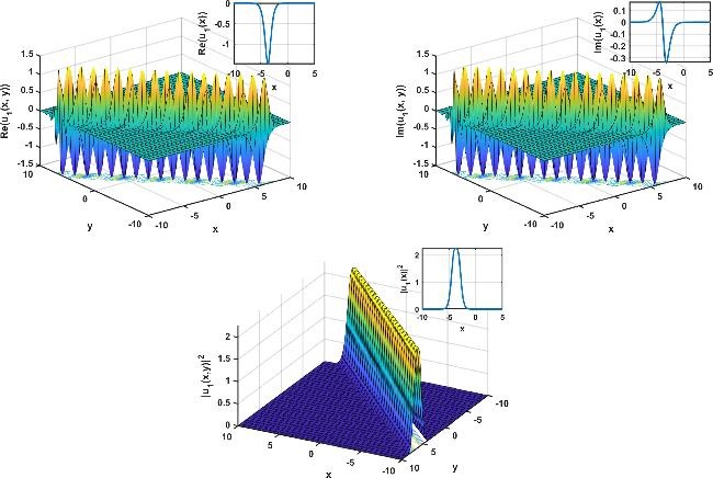
Figure 1. The profiles of equation ( |
Result 2: Consider the case r = − κ2, c = 1 − 2κ2, s = 1 − κ2, and $R\left(\vartheta \right)=\,\rm{cn}\,(\vartheta ,\kappa )$.
When ${g}_{0}=\frac{{f}_{1}}{2},{g}_{1}=0,\gamma =\frac{1+2K\beta +{w}^{2}\alpha \beta +{K}^{2}{\beta }^{2}}{{f}_{1}^{2}{w}^{2}\alpha }$, and $\,a=\frac{5-2{w}^{4}{\alpha }^{2}+10K\beta +5{w}^{2}\alpha \beta -2{K}^{2}{w}^{2}\alpha \beta +5{K}^{2}{\beta }^{2}}{4{w}^{2}\alpha }$, $\kappa \to \frac{1}{2}$, we get Jacobi function solution
$\begin{eqnarray}{u}_{2}\left(x,y,t\right)=\left(\frac{{f}_{1}}{2}+\frac{{f}_{1}\left(1-\,\rm{cn}\,{\left(\vartheta \right)}^{2}\right)}{1+\,\rm{cn}\,{\left(\vartheta \right)}^{2}}\right){{\rm{e}}}^{\,\rm{i}\,\left(-tw+Kx+ay\right)}.\end{eqnarray}$
Result 3: Consider the case r = 1, c = − 1 − κ2, s = κ2, and $R\left(\vartheta \right)=\,\rm{ns}\,(\vartheta ,\kappa )$.
When ${g}_{0}=0,{f}_{1}=0,{g}_{1}=\frac{4\sqrt{-1-2K\beta -{w}^{2}\alpha \beta -{K}^{2}{\beta }^{2}}}{w\sqrt{\alpha }\sqrt{\gamma }},$ and $a=\frac{-8-{w}^{4}{\alpha }^{2}-16K\beta -8{w}^{2}\alpha \beta -{K}^{2}{w}^{2}\alpha \beta -8{K}^{2}{\beta }^{2}}{2{w}^{2}\alpha }$, for κ → 1, then $R(\vartheta )=\coth (\vartheta )$ and we get a rational solution of hyperbolic function as shown in figure 2.
$\begin{eqnarray}\begin{array}{rcl}{u}_{3}\left(x,y,t\right) & = & \left(\frac{4\sqrt{-1-2K\beta -{w}^{2}\alpha \beta -{K}^{2}{\beta }^{2}}\coth \left(x+y-\frac{\left(-1-K\beta \right)t}{w\alpha }\right)}{w\sqrt{\alpha }\sqrt{\gamma }\left(1+{\coth \left(x+y-\frac{\left(-1-K\beta \right)t}{w\alpha }\right)}^{2}\right)}\right){{\rm{e}}}^{\,\rm{i}\,\left(-wt+Kx+\frac{\left(-8-{w}^{4}{\alpha }^{2}-16K\beta -8{w}^{2}\alpha \beta -{K}^{2}{w}^{2}\alpha \beta -8{K}^{2}{\beta }^{2}\right)y}{2{w}^{2}\alpha }\right)}.\end{array}\end{eqnarray}$
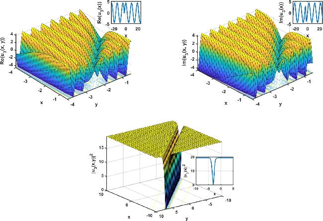
Figure 2. Plots of equation ( |
Result 4: Consider the case $r=\frac{{\kappa }^{2}}{4}$, $c=\frac{{\kappa }^{2}-2}{2}$, $s=\frac{1}{4}$, and $R(\vartheta )=\frac{\,\rm{sn}\,(\vartheta ,\kappa )}{1\mp \,\rm{dn}\,(\vartheta ,\kappa )}$.
When ${g}_{0}=0,{f}_{1}=0,{g}_{1}=-\frac{2\sqrt{-1-2K\beta -{w}^{2}\alpha \beta -{K}^{2}{\beta }^{2}}}{w\sqrt{\alpha }\sqrt{\gamma }}$, and $a=\frac{-2-{w}^{4}{\alpha }^{2}-4K\beta -2{w}^{2}\alpha \beta -{K}^{2}{w}^{2}\alpha \beta -2{K}^{2}{\beta }^{2}}{2{w}^{2}\alpha }$. For κ → 1, then $R\left(\vartheta \right)=\frac{\tanh \left(\vartheta \right)}{1\mp \,\rm{sec h}\,(\vartheta )}$, thus a combined of hyperbolic function solutions as illustrated in figure 3.
$\begin{eqnarray}\begin{array}{rcl}{u}_{4}\left(x,y,t\right) & = & \left(\frac{2\sqrt{-1-2K\beta -{w}^{2}\alpha \beta -{K}^{2}{\beta }^{2}}\tanh \left(x+y-\frac{\left(-1-K\beta \right)t}{w\alpha }\right)}{w\sqrt{\alpha }\sqrt{\gamma }\left(1+\,\rm{sech}\,\left(x+y-\frac{\left(-1-K\beta \right)t}{w\alpha }\right)\right)(1+\frac{{\tanh \left(x+y-\frac{\left(-1-K\beta \right)t}{w\alpha }\right)}^{2}}{{\left(1+\,\rm{sech}\,\left(x+y-\frac{\left(-1-K\beta \right)t}{w\alpha }\right)\right)}^{2}})}\right)\\ & & \times {{\rm{e}}}^{\,\rm{i}\,\left(-wt+Kx+\frac{\left(-2-{w}^{4}{\alpha }^{2}-4K\beta -2{w}^{2}\alpha \beta -{K}^{2}{w}^{2}\alpha \beta -2{K}^{2}{\beta }^{2}\right)y}{2{w}^{2}\alpha }\right)}.\end{array}\end{eqnarray}$
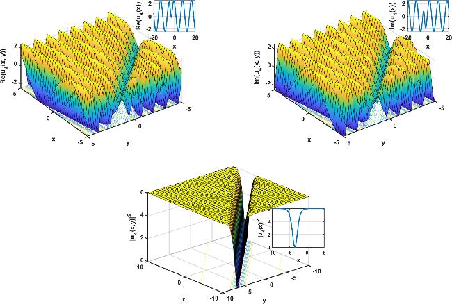
Figure 3. Profiles of equation ( |
Result 5: Consider the case r = − 1, c = 2 − κ2, s = − 1 + κ2, and $R\left(\vartheta \right)={\rm{d}}{\rm{n}}\vartheta ,\kappa )$. When ${g}_{0}=0,{g}_{1}=-2{\rm{i}}{f}_{1},\gamma =\frac{-1-2K\beta -{\omega }^{2}\alpha \beta -{K}^{2}{\beta }^{2}}{{f}_{1}^{2}{\omega }^{2}\alpha }$ and $a=\frac{2-{\omega }^{4}{\alpha }^{2}+4K\beta +2{\omega }^{2}\alpha \beta -{K}^{2}{\omega }^{2}\alpha \beta +2{K}^{2}{\beta }^{2}}{2{\omega }^{2}\alpha }$. For κ → 0, we have $R\left(\vartheta \right)=1$ and we get an exponential function solution.
$\begin{eqnarray}{u}_{5}\left(x,y,t\right)=(-\,\rm{i}\,{f}_{1}){{\rm{e}}}^{\,\rm{i}\,\left(-wt+Kx+\frac{\left(2-{w}^{4}{\alpha }^{2}+4K\beta +2{w}^{2}\alpha \beta -{K}^{2}{w}^{2}\alpha \beta +2{K}^{2}{\beta }^{2}\right)y}{2{w}^{2}\alpha }\right)}.\end{eqnarray}$
4. The Biswas–Milovic equation and its optical solutions
In this section, the JEFEM is employed to construct optical solutions of the BME. Consider the BME with power law non linearity i.e. F(Ω) = Ω2, then equation (2 ) takes the following form [50]: 20 ) to (19 ), yields 2 ) is formulated with a general non-Kerr nonlinearity $F\,\left(| S{| }^{2}\right)$, in the present study we restrict our attention to the Kerr-type case $F\,\left(| S{| }^{2}\right)=| S{| }^{2}$. This assumption is introduced in order to obtain a polynomial reduced ordinary differential equation, which is a necessary requirement for the effective implementation of the Jacobi elliptic function expansion method. Under this Kerr-type nonlinearity, the reduced equation naturally leads to the quartic nonlinear term βU4 appearing in equation (22 ). Consequently, the exact solutions derived in this work are valid for the BME with cubic (Kerr) nonlinearity. For more general non-Kerr laws, such as power-law or saturable nonlinearities, the reduced equation becomes non-polynomial, and the Jacobi elliptic function expansion method cannot be applied directly without further modifications or approximations, which are beyond the scope of the present study.
$\begin{eqnarray}{{\rm{i}}({S}^{n})}_{t}-\alpha ({({S}^{n})}_{xx}+{({S}^{n})}_{yy})-(\beta \,{\left|S\right|}^{2n}-M){S}^{n}=0.\end{eqnarray}$
Starting from the transformation $\begin{eqnarray}S\left(x,y,t\right)={{\rm{e}}}^{{\rm{i}}\phi \left(x,y,t\right)}U\left(\vartheta \right),\,\vartheta =ax+by+\omega t,\,\phi \left(x,y,t\right)=x+y+vt,\end{eqnarray}$
where $U\left(\vartheta \right)$ is a real valued function, a, b are wave number in x and y direction, respectively. While w stands for wave speed and v represent the temporal oscillations. Inserting equation ( $\begin{eqnarray}\begin{array}{l}-(M+n(2n\alpha -v){U}^{2})+\beta \,{U}^{4}+({a}^{2}+{b}^{2})(n-1)\alpha n{(U^{\prime} )}^{2}+n({\rm{i}}(2(a+b)n\alpha -\omega )UU^{\prime} +\alpha ({a}^{2}+{b}^{2})U^{\prime\prime} )=0.\end{array}\end{eqnarray}$
Although equation (The subsequent sections of equation (21 ) are denoted as follows. The real part is
$\begin{eqnarray}\begin{array}{l}-((M+n(2n\alpha -a){U}^{2})+\beta \,{U}^{4}+n\alpha ({a}^{2}+{b}^{2})(n-1){(U^{\prime} )}^{2}+n\alpha ({a}^{2}+{b}^{2})UU^{\prime\prime} =0.\end{array}\end{eqnarray}$
The imaginary part is $\begin{eqnarray}n((2(a+b)n\alpha -\omega ))UU^{\prime} =0.\end{eqnarray}$
Next, by setting the imaginary part's elemental coefficients to zero, we have $a=\frac{-2bn\alpha +\omega }{2n\alpha },$ where nα ≠ 0. Utilizing the balance principle to achieve M = 1, refer to equation (6 ) to articulate the solution of equation (12 ) as follows.
$\begin{eqnarray}G\left(\vartheta \right)={g}_{0}+{g}_{1}\frac{R\left(\vartheta \right)}{1+R{\left(\vartheta \right)}^{2}}+{f}_{1}\frac{1-R{\left(\vartheta \right)}^{2}}{1+R{\left(\vartheta \right)}^{2}}.\end{eqnarray}$
Inserting equation (24 ) into (22 ), then the following set of algebraic equations will be acquired:
\begin{array}{l}\text { Constants: }-f_{1}^{2} M-2 f_{1} g_{0} M-g_{0}^{2} M+n v f_{1}^{2}+2 v n f_{1} g_{0}+v n g_{0}^{2}-2 f_{1}^{2} n^{2} \alpha-4 f_{1} g_{0} n^{2} \alpha-2 g_{0}^{2} n^{2} \alpha \\-4 a^{2} f_{1}^{2} n s \alpha-4 b^{2} f_{1}^{2} n s \alpha-4 a^{2} f_{1} g_{0} n s \alpha-4 b^{2} f_{1} g_{0} n s \alpha-a^{2} g_{1}^{2} n s \alpha-b^{2} g_{1}^{2} n s \alpha+a^{2} g_{1}^{2} n^{2} s \alpha+b^{2} g_{1}^{2} n^{2} s \alpha \\+f_{1}^{4} \beta+4 f_{1}^{3} g_{0} \beta+6 f_{1}^{2} g_{0}^{2} \beta+4 f_{1} g_{0}^{3} \beta+g_{0}^{4} \beta=0, \\R(\vartheta):-2 f_{1} g_{1} M-2 g_{0} g_{1} M+2 v n f_{1} g_{1}+2 v n g_{0} g_{1}+a^{2} c f_{1} g_{1} n \alpha+b^{2} c f_{1} g_{1} n \alpha+a^{2} c g_{0} g_{1} n \alpha+b^{2} c g_{0} g_{1} n \alpha \\-4 f_{1} g_{1} n^{2} \alpha-4 g_{0} g_{1} n^{2} \alpha-2 a^{2} f_{1} g_{1} n s \alpha-2 b^{2} f_{1} g_{1} n s \alpha-6 a^{2} g_{0} g_{1} n s \alpha-6 b^{2} g_{0} g_{1} n s \alpha-8 a^{2} f_{1} g_{1} n^{2} s \alpha \\-8 b^{2} f_{1} g_{1} n^{2} s \alpha+4 f_{1}^{3} g_{1} \beta+12 f_{1}^{2} g_{0} g_{1} \beta+12 f_{1} g_{0}^{2} g_{1} \beta+4 g_{0}^{3} g_{1} \beta=0, \\R(\vartheta)^{2}:-4 f_{1} g_{0} M-4 g_{0}^{2} M-g_{1}^{2} M+4 v n f_{1} g_{0}+4 v n g_{0}^{2}+v n g_{1}^{2}-8 a^{2} c f_{1}^{2} n \alpha-8 b^{2} c f_{1}^{2} n \alpha-8 a^{2} c f_{1} g_{0} n \alpha \\-8 b^{2} c f_{1} g_{0} n \alpha-8 f_{1} g_{0} n^{2} \alpha-8 g_{0}^{2} n^{2} \alpha-2 g_{1}^{2} n^{2} \alpha+a^{2} c g_{1}^{2} n^{2} \alpha+b^{2} c g_{1}^{2} n^{2} \alpha+8 a^{2} f_{1} g_{0} n s \alpha+8 b^{2} f_{1} g_{0} n s \alpha \\-4 a^{2} g_{1}^{2} n s \alpha-4 b^{2} g_{1}^{2} n s \alpha+16 a^{2} f_{1}^{2} n^{2} s \alpha+16 b^{2} f_{1}^{2} n^{2} s \alpha-2 a^{2} g_{1}^{2} n^{2} s \alpha-2 b^{2} g_{1}^{2} n^{2} s \alpha-4 f_{1}^{4} \beta \\-8 f_{1}^{3} g_{0} \beta+8 f_{1} g_{0}^{3} \beta+4 g_{0}^{4} \beta+6 f_{1}^{2} g_{1}^{2} \beta+12 f_{1} g_{0} g_{1}^{2} \beta+6 g_{0}^{2} g_{1}^{2} \beta=0, \\R(\vartheta)^{3}:-2 f_{1} g_{1} M-6 g_{0} g_{1} M+2 v n f_{1} g_{1}+6 v n g_{0} g_{1}-7 a^{2} c f_{1} g_{1} n \alpha-7 b^{2} c f_{1} g_{1} n \alpha-5 a^{2} c g_{0} g_{1} n \alpha-5 b^{2} c g_{0} g_{1} n \alpha \\-4 f_{1} g_{1} n^{2} \alpha-8 a^{2} c f_{1} g_{1} n^{2} \alpha-8 b^{2} c f_{1} g_{1} n^{2} \alpha-12 g_{0} g_{1} n^{2} \alpha+2 a^{2} f_{1} g_{1} n r \alpha+2 b^{2} f_{1} g_{1} n r \alpha+2 a^{2} g_{0} g_{1} n r \alpha \\+\left.2 b\right|^{2} g_{0} g_{1} n r \alpha+12 a^{2} f_{1} g_{1} n s \alpha+12 b^{2} f_{1} g_{1} n s \alpha-4 a^{2} g_{0} g_{1} n s \alpha-4 b^{2} g_{0} g_{1} n s \alpha+8 a^{2} f_{1} g_{1} n^{2} s \alpha \\+8 b^{2} f_{1} g_{1} n^{2} s \alpha-12 f_{1}^{3} g_{1} \beta-12 f_{1}^{2} g_{0} g_{1} \beta+12 f_{1} g_{0}^{2} g_{1} \beta+12 g_{0}^{3} g_{1} \beta+4 f_{1} g_{1}^{3} \beta+4 g_{0} g_{1}^{3} \beta=0 \\R(\vartheta)^{4}: 2 f_{1}^{2} M-6 g_{0}^{2} M-2 g_{1}^{2} M-2 v n f_{1}^{2}+6 v n g_{0}^{2}+2 v n g_{1}^{2}-4 a^{2} c g_{1}^{2} n \alpha-4 b^{2} c g_{1}^{2} n \alpha+4 f_{1}^{2} n^{2} \alpha \\+16 a^{2} c f_{1}^{2} n^{2} \alpha+16 b^{2} c f_{1}^{2} n^{2} \alpha-12 g_{0}^{2} n^{2} \alpha-4 g_{1}^{2} n^{2} \alpha-2 a^{2} c g_{1}^{2} n^{2} \alpha-2 b^{2} c g_{1}^{2} n^{2} \alpha-12 a^{2} f_{1}^{2} n r \alpha \\-12 b^{2} f_{1}^{2} n r \alpha-12 a^{2} f_{1} g_{0} n r \alpha-12 b^{2} f_{1} g_{0} n r \alpha+a^{2} g_{1}^{2} n r \alpha+b^{2} g_{1}^{2} n r \alpha+a^{2} g_{1}^{2} n^{2} r \alpha+b^{2} g_{1}^{2} n^{2} r \alpha \\-12 a^{2} f_{1}^{2} n s \alpha-12 b^{2} f_{1}^{2} n s \alpha+12 a^{2} f_{1} g_{0} n s \alpha+12 b^{2} f_{1} g_{0} n s \alpha+a^{2} g_{1}^{2} n s \alpha+b^{2} g_{1}^{2} n s \alpha+a^{2} g_{1}^{2} n^{2} s \alpha \\+b^{2} g_{1}^{2} n^{2} s \alpha+6 f_{1}^{4} \beta-12 f_{1}^{2} g_{0}^{2} \beta+6 g_{0}^{4} \beta-12 f_{1}^{2} g_{1}^{2} \beta+12 g_{0}^{2} g_{1}^{2} \beta+g_{1}^{4} \beta=0, \\R(\vartheta)^{5}: 2 f_{1} g_{1} M-6 g_{0} g_{1} M-2 v n f_{1} g_{1}+6 v n g_{0} g_{1}+7 a^{2} c f_{1} g_{1} n \alpha+7 b^{2} c f_{1} g_{1} n \alpha-5 a^{2} c g_{0} g_{1} n \alpha-5 b^{2} c g_{0} g_{1} n \alpha \\+4 f_{1} g_{1} n^{2} \alpha+8 a^{2} c f_{1} g_{1} n^{2} \alpha+8 b^{2} c f_{1} g_{1} n^{2} \alpha-12 g_{0} g_{1} n^{2} \alpha-12 a^{2} f_{1} g_{1} n r \alpha-12 b^{2} f_{1} g_{1} n r \alpha-4 a^{2} g_{0} g_{1} n r \alpha \\-4 b^{2} g_{0} g_{1} n r \alpha-8 a^{2} f_{1} g_{1} n^{2} r \alpha-8 b^{2} f_{1} g_{1} n^{2} r \alpha-2 a^{2} f_{1} g_{1} n s \alpha-2 b^{2} f_{1} g_{1} n s \alpha+2 a^{2} g_{0} g_{1} n s \alpha+2 b^{2} g_{0} g_{1} n s \alpha \\+12 f_{1}^{3} g_{1} \beta-12 f_{1}^{2} g_{0} g_{1} \beta-12 f_{1} g_{0}^{2} g_{1} \beta+12 g_{0}^{3} g_{1} \beta-4 f_{1} g_{1}^{3} \beta+4 g_{0} g_{1}^{3} \beta=0, \\R(\vartheta)^{6}: 4 f_{1} g_{0} M-4 g_{0}^{2} M-g_{1}^{2} M-4 v n f_{1} g_{0}+4 v n g_{0}^{2}+v n g_{1}^{2}-8 a^{2} c f_{1}^{2} n \alpha-8 b^{2} c f_{1}^{2} n \alpha+8 a^{2} c f_{1} g_{0} n \alpha \\+8 b^{2} c f_{1} g_{0} n \alpha+8 f_{1} g_{0} n^{2} \alpha-8 g_{0}^{2} n^{2} \alpha-2 g_{1}^{2} n^{2} \alpha+a^{2} c g_{1}^{2} n^{2} \alpha+b^{2} c g_{1}^{2} n^{2} \alpha-8 a^{2} f_{1} g_{0} n r \alpha-8 b^{2} f_{1} g_{0} n r \alpha \\-4 a^{2} g_{1}^{2} n r \alpha-4 b^{2} g_{1}^{2} n r \alpha+16 a^{2} f_{1}^{2} n^{2} r \alpha+16 b^{2} f_{1}^{2} n^{2} r \alpha-2 a^{2} g_{1}^{2} n^{2} r \alpha-2 b^{2} g_{1}^{2} n^{2} r \alpha-4 f_{1}^{4} \beta+8 f_{1}^{3} g_{0} \beta \\-8 f_{1} g_{0}^{3} \beta+4 g_{0}^{4} \beta+6 f_{1}^{2} g_{1}^{2} \beta-12 f_{1} g_{0} g_{1}^{2} \beta+6 g_{0}^{2} g_{1}^{2} \beta=0, \\R(\vartheta)^{7}: 2 f_{1} g_{1} M-2 g_{0} g_{1} M-2 v n f_{1} g_{1}+2 v n g_{0} g_{1}-a^{2} c f_{1} g_{1} n \alpha-b^{2} c f_{1} g_{1} n \alpha+a^{2} c g_{0} g_{1} n \alpha+b^{2} c g_{0} g_{1} n \alpha \\+4 f_{1} g_{1} n^{2} \alpha-4 g_{0} g_{1} n^{2} \alpha+2 a^{2} f_{1} g_{1} n r \alpha+2 b^{2} f_{1} g_{1} n r \alpha-6 a^{2} g_{0} g_{1} n r \alpha-6 b^{2} g_{0} g_{1} n r \alpha+8 a^{2} f_{1} g_{1} n^{2} r \alpha \\+8 b^{2} f_{1} g_{1} n^{2} r \alpha-4 f_{1}^{3} g_{1} \beta+12 f_{1}^{2} g_{0} g_{1} \beta-12 f_{1} g_{0}^{2} g_{1} \beta+4 g_{0}^{3} g_{1} \beta=0, \\R(\vartheta)^{8}:-f_{1}^{2} M+2 f_{1} g_{0} M-g_{0}^{2} M+v n f_{1}^{2}-2 v n f_{1} g_{0}+v n g_{0}^{2}-2 f_{1}^{2} n^{2} \alpha+4 f_{1} g_{0} n^{2} \alpha-2 g_{0}^{2} n^{2} \alpha-4 a^{2} f_{1}^{2} n r \alpha \\-4 b^{2} f_{1}^{2} n r \alpha+4 a^{2} f_{1} g_{0} n r \alpha+4 b^{2} f_{1} g_{0} n r \alpha-a^{2} g_{1}^{2} n r \alpha-b^{2} g_{1}^{2} n r \alpha+a^{2} g_{1}^{2} n^{2} r \alpha+b^{2} g_{1}^{2} n^{2} r \alpha+f_{1}^{4} \beta \\-4 f_{1}^{3} g_{0} \beta+6 f_{1}^{2} g_{0}^{2} \beta-4 f_{1} g_{0}^{3} \beta+g_{0}^{4} \beta=0,\end{array}
Utilizing computer software to resolve the previous mathematical system could give different results:
Result 1: Consider the case r = κ2, c = − 1 − κ2, s = 1 and $R\left(\vartheta \right)=\,\rm{sn}\,(\vartheta ,\kappa )$.
When ${g}_{0}=0,{g}_{1}=0,\beta =\frac{4n\alpha ({a}^{2}+{b}^{2})(n+1)}{{f}_{1}^{2}},$ $M=n(v-2n\alpha +4{a}^{2}n\alpha +4{b}^{2}n\alpha )$, and when κ → 1, then $R(\vartheta )=\tanh (\vartheta )$, we get rational solution of dark solitary wave as shown in (figure 4).
$\begin{eqnarray}{S}_{1}\left(x,y,t\right)=\frac{{f}_{1}\left(1-\,\rm{tanh}\,{\left(\frac{-2bn\alpha +\omega }{2n\alpha }x+by+\omega t\right)}^{2}\right)}{1+\,\rm{tanh}\,{\left(\frac{-2bn\alpha +\omega }{2n\alpha }x+by+\omega t\right)}^{2}}{{\rm{e}}}^{{\rm{i}}\left(x+y+vt\right)}.\end{eqnarray}$
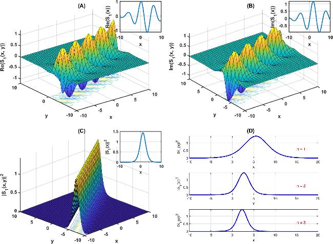
Figure 4. (A) Real part (B) imaginary part (C) Abs plot (D) 2D of S1(x) of equation ( |
Result 2: Consider the case r = 1, c = − 1 − κ2, s = κ2 and $R\left(\vartheta \right)=\,\rm{ns}\,(\vartheta ,\kappa )$.
When ${g}_{0}=0,{g}_{1}=0,{f}_{1}=\frac{2\sqrt{{a}^{2}+{b}^{2}}\sqrt{n}\sqrt{n+1}\sqrt{\alpha }}{\sqrt{\beta }},$ $M=n(v-2n\alpha +4{a}^{2}n\alpha +4{b}^{2}n\alpha )$, and when κ → 1, then $R(\vartheta )=\coth (\vartheta )$, we get a rational solution of hyperbolic function (figure 5).
$\begin{eqnarray}{S}_{2}\left(x,y,t\right)=\frac{2\sqrt{n}\sqrt{1+n}\sqrt{\alpha }\sqrt{{b}^{2}+\frac{{(-2bn\alpha +\omega )}^{2}}{4{n}^{2}{\alpha }^{2}}}\left(1-\,\rm{coth}\,{\left(\frac{-2bn\alpha +\omega }{2n\alpha }x+by+\omega t\right)}^{2}\right)}{\sqrt{\beta }\left(1+\,\rm{coth}\,{\left(\frac{-2bn\alpha +\omega }{2n\alpha }x+by+\omega t\right)}^{2}\right)}{{\rm{e}}}^{{\rm{i}}\left(x+y+vt\right)}.\end{eqnarray}$
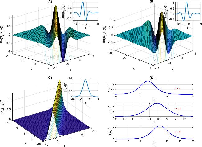
Figure 5. (A) Real part (B) imaginary part (C) Abs plot (D) 2D of S2(x) of equation ( |
Result 3: Consider the case $r=\frac{1}{4},c=\frac{1-2{\kappa }^{2}}{2},s=\frac{1}{4}$ and $R\left(\vartheta \right)=\,\rm{ns}\,(\vartheta ,\kappa )+\,\rm{cs}\,(\vartheta ,\kappa )$.
When ${g}_{0}=0,{g}_{1}=0,{f}_{1}=\frac{\sqrt{{a}^{2}+{b}^{2}}\sqrt{n}\sqrt{n+1}\sqrt{\alpha }}{\sqrt{\beta }},$ $M=n(v-2n\alpha +{a}^{2}n\alpha +{b}^{2}n\alpha )$, and when κ → 1, then R(ϑ) = coth(ϑ) + csch(ϑ), we have a rational solution of combined hyperbolic function (figure 6).
$\begin{eqnarray}\begin{array}{rlr}{S}_{3}\left(x,y,t\right)\,= & \frac{\sqrt{n}\sqrt{1+n}\sqrt{\alpha }\sqrt{{b}^{2}+\frac{{(-2bn\alpha +\omega )}^{2}}{4{n}^{2}{\alpha }^{2}}}\left(1-{\left(\coth \left(\frac{-2bn\alpha +\omega }{2n\alpha }x+by+\omega t\right)+\,\rm{csch}\,\left(\frac{-2bn\alpha +\omega }{2n\alpha }x+by+\omega t\right)\right)}^{2}\right)}{\sqrt{\beta }\left(1+{\left(\,\rm{coth}\,\left(\frac{-2bn\alpha +\omega }{2n\alpha }x+by+\omega t\right)+\,\rm{csch}\,\left(\frac{-2bn\alpha +\omega }{2n\alpha }x+by+\omega t\right)\right)}^{2}\right)} & \\ & \times {{\rm{e}}}^{{\rm{i}}\left(x+y+vt\right)}.\end{array}\end{eqnarray}$
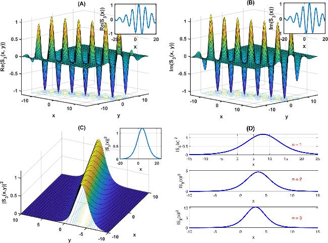
Figure 6. (A) Real part (B) imaginary part (C) Abs plot (D) 2D of S3(x) of equation ( |
Result 4: Consider the case $r=\frac{1-{\kappa }^{2}}{4},c=\frac{{\kappa }^{2}+1}{2},s=\frac{1-{\kappa }^{2}}{4}$ and $R\left(\vartheta \right)=\,\rm{nc}\,(\vartheta ,\kappa )+\,\rm{sc}\,(\vartheta ,\kappa )$.
When ${g}_{0}=0,{f}_{1}=0,{g}_{1}=\frac{2\sqrt{{a}^{2}+{b}^{2}}\sqrt{n}\sqrt{n+1}\sqrt{\alpha }}{\sqrt{\beta }},$ $M=n(v-2n\alpha +{a}^{2}n\alpha +{b}^{2}n\alpha )$, and when κ → 1, then R(ϑ) = sinh(ϑ) + cosh(ϑ), we get a rational solution of combined hyperbolic function (figure 7).
$\begin{eqnarray}\begin{array}{rlr}{S}_{4}\left(x,y,t\right)= & \frac{2\sqrt{n}\sqrt{1+n}\sqrt{\alpha }\sqrt{{b}^{2}+\frac{{(-2bn\alpha +\omega )}^{2}}{4{n}^{2}{\alpha }^{2}}}\left({\rm{\cosh }}\left(\frac{-2bn\alpha +\omega }{2n\alpha }x+by+\omega t\right)+{\rm{\sinh }}\left(\frac{-2bn\alpha +\omega }{2n\alpha }x+by+\omega t\right)\right)}{\sqrt{\beta }\left(1+{\left({\rm{\cosh }}\left(\frac{-2bn\alpha +\omega }{2n\alpha }x+by+\omega t\right)+{\rm{\sinh }}\left(\frac{-2bn\alpha +\omega }{2n\alpha }x+by+\omega t\right)\right)}^{2}\right)} & \\ & \times {{\rm{e}}}^{{\rm{i}}\left(x+y+vt\right)}.\end{array}\end{eqnarray}$
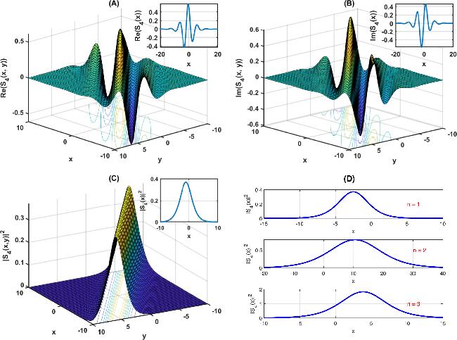
Figure 7. (A) Real part (B) imaginary part (C) Abs plot (D) 2D of S4(x) of equation ( |
Result 5: In the case $r=\frac{{\kappa }^{2}}{4},c=\frac{{\kappa }^{2}-2}{2},s=\frac{1}{4}$ and $R(\vartheta )=\frac{\,\rm{sn}\,(\vartheta ,\kappa )}{1\mp {\rm{d}}{\rm{n}}(\vartheta ,\kappa )}$. When ${g}_{0}=0,{g}_{1}=0,{f}_{1}=\frac{\sqrt{{a}^{2}+{b}^{2}}\sqrt{n}\sqrt{n+1}\sqrt{\alpha }}{\sqrt{\beta }},$ $M=n(v-2n\alpha +{a}^{2}n\alpha +{b}^{2}n\alpha )$, and for κ → 1, we have $R(\vartheta )=\frac{\,\rm{tanh}\,(\vartheta ,\kappa )}{1\mp \,\rm{sech}\,(\vartheta ,\kappa )}$ and get a rational solution of the combined dark–bright solitary wave as seen in (figure 8).
$\begin{eqnarray}{S}_{5}\left(x,y,t\right)=\frac{\sqrt{n}\sqrt{1+n}\sqrt{\alpha }\sqrt{{b}^{2}+\frac{{(-2bn\alpha +\omega )}^{2}}{4{n}^{2}{\alpha }^{2}}}\left(1-\frac{\tanh {\left(\frac{-2bn\alpha +\omega }{2n\alpha }x+by+\omega t\right)}^{2}}{{\left(1+\,\rm{sech}\,\left(\frac{-2bn\alpha +\omega }{2n\alpha }x+by+\omega t\right)\right)}^{2}}\right)}{\sqrt{\beta }\left(1+\frac{\tanh {\left(\frac{-2bn\alpha +\omega }{2n\alpha }x+by+\omega t\right)}^{2}}{{\left(1+\,\rm{sech}\,\left(\frac{-2bn\alpha +\omega }{2n\alpha }x+by+\omega t\right)\right)}^{2}}\right)}{{\rm{e}}}^{{\rm{i}}\left(x+y+vt\right)}.\end{eqnarray}$
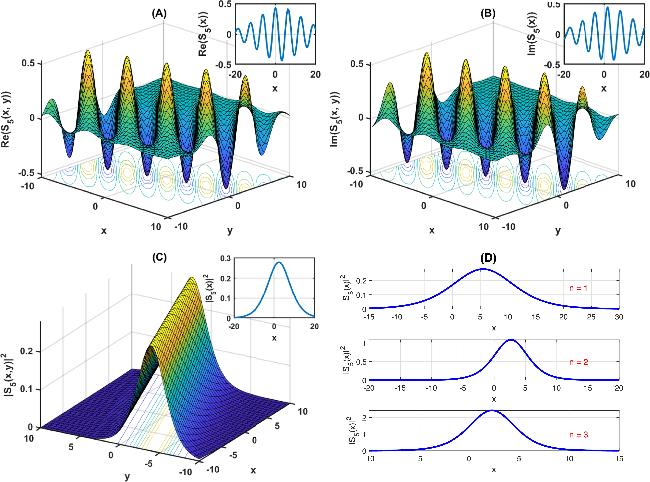
Figure 8. (A) Real part (B) imaginary part (C) Abs plot (D) 2D of S5(x) of equation ( |
Result 6: In the case r = 1 − κ2, c = 2 − κ2, s = 1 and R(ϑ) = sc(ϑ, κ). When ${g}_{0}=\frac{\sqrt{2}\sqrt{{a}^{2}n\alpha +{b}^{2}n\alpha }}{\sqrt{\beta }},{g}_{1}=0,{f}_{1}=0,$ $M=-n(-v-2{a}^{2}\alpha -2{b}^{2}\alpha +2n\alpha )$, and for κ → 1, we have R(ϑ) = tan(ϑ, κ) and get a constant function.
$\begin{eqnarray}{S}_{6}\left(x,y,t\right)=\frac{\sqrt{2}\sqrt{{b}^{2}n\alpha +\frac{{(-2bn\alpha +\omega )}^{2}}{4n\alpha }}}{\sqrt{\beta }}{{\rm{e}}}^{{\rm{i}}\left(x+y+vt\right)}.\end{eqnarray}$
Result 7: In the case $r=\frac{1}{4},c=\frac{{\kappa }^{2}-2}{2},s=\frac{{\kappa }^{4}}{4}$ and R(ϑ) = ns(ϑ, κ) ∓ ds(ϑ, κ). When ${g}_{0}=0,{g}_{1}=0,{f}_{1}=\frac{\sqrt{{a}^{2}+{b}^{2}}\sqrt{n}\sqrt{n+1}\sqrt{\alpha }}{\sqrt{\beta }},$ $M=n(v-2n\alpha +{a}^{2}n\alpha +{b}^{2}n\alpha )$, and for κ → 1, we have $R(\vartheta )=\coth (\vartheta )\mp \,\rm{csch}\,(\vartheta )$ and get a rational solution of the combined singular solitary wave as shown in figure 9.
$\begin{eqnarray}\begin{array}{rlr}{S}_{7}\left(x,y,t\right)\,= & \frac{\sqrt{n}\sqrt{1+n}\sqrt{\alpha }\sqrt{{b}^{2}+\frac{{(-2bn\alpha +\omega )}^{2}}{4{n}^{2}{\alpha }^{2}}}\left(1-{\left(\coth \left(\frac{-2bn\alpha +\omega }{2n\alpha }x+by+\omega t\right)+\,\rm{csch}\,\left(\frac{-2bn\alpha +\omega }{2n\alpha }x+by+\omega t\right)\right)}^{2}\right)}{\sqrt{\beta }\left(1+{\left(\coth \left(\frac{-2bn\alpha +\omega }{2n\alpha }x+by+\omega t\right)+\,\rm{csch}\,\left(\frac{-2bn\alpha +\omega }{2n\alpha }x+by+\omega t\right)\right)}^{2}\right)} & \\ & \times {{\rm{e}}}^{{\rm{i}}\left(x+y+vt\right)}.\end{array}\end{eqnarray}$
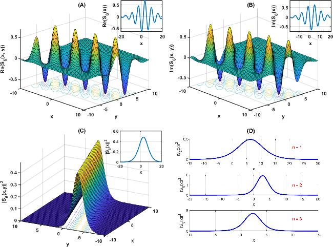


Figure 9. (A) Real part (B) imaginary part (C) Abs plot (D) 2D of S7(x) of equation ( |
5. Results and discussion
The obtained solutions express a range of wave structures such as dark soliton, singular soliton, periodic waves, and combined dark–bright profiles. The nonlinear structure of the governing equations and the adaptability of the Jacobi elliptic function expansion approach give rise to these many solution variants. These structures are frequently seen in optical fibers and wave guides, where the wave dynamics are shaped by the interaction of dispersion, diffraction, and non linearity.
Additionally, the graphical representations show that the physical parameters, such as the dispersion coefficient, nonlinearity strength, and wave velocity, have a significant impact on the amplitude and shape of the solutions. Changes in these parameters alter the soliton profiles' width and intensity, suggesting potential ways to regulate wave propagation in real-world optical systems. The two-dimensional charts show how important the nonlinear parameter n is in determining the stability and evolution of the solutions for the BME. These discoveries underline the physical importance of the presented results and their possible applicability in nonlinear optics.
Figure 1 depicts the solution of equation (14 ) which represents a dark solution, the parameters are specified as (α = 0.25, K = 0.5, f1 = 1.5, w = 1.2, β = 0.2, and t = 1). Figure 2 illustrates the solution of equation (16 ) that describes a rational solution of a hyperbolic function, the parameters are selected as (α = 0.28, K = 0.65, f1 = 1.8, w = 1.4, β = 0.3, γ = 0.6 and t = 1). Figure 3 donates the solution of equation (17 ) which is a rational solution of combination hyperbolic function, the parameters are given as (α = 0.34, K = 0.76, g1 = 1.8, w = 1.1, β = 0.4, γ = 0.74 and t = 1). Figure 4 illustrates the solution of equation (25 ), which represents by a rational solution of a dark solitary wave, the parameters are chosen as (α = 0.56, β = 0.78, ω = 0.32, b = 0.42, f1 = 1.2, n = 1, and t = 1). Figure 5 gives the solution of equation (26 ), which is a rational of singular solution, the parameters are chosen as (α = 0.54, β = 0.53, ω = 0.62, b = 0.32, n = 1, and t = 1). Figure 6 illustrates the solution of equation (27 ), whch is a combination of rational singular solution, the parameters are set to (α = 0.81, β = 0.38, ω = 0.6, b = 0.51, n = 1 and t = 1). Figure 7 represents the solution of equation (28 ), the parameters are set to (α = 0.21, β = 0.48, ω = 0.38, b = 0.54, n = 1, and t = 1). Figure 8 represents the solution of equation (29 ) which describes a rational solution of combination dark–bright solitary wave, the parameters are set to (α = 0.56, β = 0.78, ω = 0.32, b = 0.42, n = 1, and t = 1). Figure 9 represents the solution of equation (30 ), which describes as a rational solution of the combination of dark–bright solitary wave the parameters are set to (α = 0.5, β = 0.85, ω = 0.45, b = 0.62, n = 1, and t = 1).
The DTDPE and the BME have been studied previously using a variety of analytical methods, under certain parameter constraints, these methods have mostly yielded restricted classes of soliton or periodic solutions. In contrast, a wider variety of exact solutions, such as dark solitons, singular solitons, periodic, and combined hyperbolic function solutions, are constructed in the current study using the Jacobi elliptic expansion function method within a single framework. This comparison illustrates both the originality of the results achieved and the efficacy of the proposed approach. Comparing our results with [39–65], we deduce that our solutions are new and have different categories.
6. Conclusion
In this article, we provide new applications of the Jacobi elliptic function expansion approach to obtain new optical solutions for the DTDPE and the BME. This work's primary contribution is the derivation of new classes of exact solutions inside a single framework, such as dark soliton, singular soliton, periodic, and coupled hyperbolic function solutions. By offering a wider class of wave shapes and a better understanding of the function of physical parameters, the acquired results expand upon previous analytical investigations. These results provide prospective applications in nonlinear optics and fiber optic systems, in addition to improving the theoretical knowledge of nonlinear wave equations. This approach is strong, dependable, and efficient for solving the NPDEs. Moreover, graphic representations in two and three dimensions have been created to illustrate the physical behavior of the obtained results, also for BME we create the two dimensions figure under the effect of nonlinear parameter. The results are significant in interpreting the physical implications of the NPDEs. The proposed method show promise in solving other nonlinear equations as well. In our future work, we will try to apply the Jacobi elliptic function expansion method to investigate some NPDEs with variable coefficients.