

1. Introduction
Linear non-Hermitian systems have recently attracted significant attention due to their rich physical phenomena, including nontrivial topology [1–4], enhanced sensitivity near exceptional points in the spectra [5], and the non-Hermitian skin effect [6–8]. Interestingly, localized wave states in nonlinear Hermitian systems can exhibit non-orthogonality and merge at the degeneracy points of soliton excitation energies [9–12], which is very similar to the eigenstates of linear non-Hermitian systems [6]. These suggest that there could be some intrinsic relations between nonlinear Hermitian systems and linear non-Hermitian systems. Very recently, some quantitative relations between them were uncovered for some well-known nonlinear Schrödinger (NLS) equations [13], with the aid of Lax integrability theory.
For the simple NLS models, the degeneracies of the real or imaginary spectrum of the linear non-Hermitian matrices are uncovered to clarify several essential characteristics of nonlinear localized waves, such as breathers, rogue waves (RWs), and solitons [13]. It has been found that the exceptional points (EPs) generally correspond to RWs for modulational instability (MI) cases and to dark solitons with maximum velocity for the modulational stability (MS) cases. However, there are many high-order effects in nonlinear systems, such as third-order dispersion, self-steepening, and delayed nonlinear response, etc., which can not be ignored for short pulse or higher power pulse [14, 15]. This motivates scientists to construct modified NLSs with taking these high-order effects. The Sasa-Satsuma (S–S) equation is one of the most important integrable extensions, and this system exhibits many dynamic phenomena that are different from the standard NLS system, such as W-shaped solitons (WSs) [16–18] and W-shaped soliton trains (WSTs) [19, 20]. Linear stability analysis of the plane waves indicates that there is a MS gap in the MI regime [21], which is always absent for the NLS model. This striking character make the S–S model admit more abundant nonlinear waves. For example, RW and WS emerge simultaneously at the boundary between MI and MS. [21], for which the dynamics process involves both MI and MS. These characters hint that the quantitative relations for S–S model could admit some new characters being absent for NLS model.
On the other hand, the linear stability analysis generally admit non-Hermitian forms, which are distinct from the ones given by Lax-pairs. The quantitative relations between MI and nonlinear waves have been established for many different nonlinear systems [21–24]. The real and imaginary parts of the spectra on the resonance line even determine the spatial-temporal pattern of RWs [25, 26]. The perturbation eigenvector can be used to relate to the types of nonlinear waves, in contrast to that the spectral parameter play essential role for the Lax-pair analysis cases. These results provide possibilities to obtain the correspondence between the two different linear non-Hermitian models for one identical nonlinear Hermitian system, which could greatly deepen our realization on the intrinsic relations between these distinctive aspects.
In this work, we expand the quantitative correspondence between the degeneracies of the linear non-Hermitian matrices and the localized wave solutions of nonlinear Hermitian systems. We analyze the eigenvalue degeneracy of Lax-pairs in detail. The eigenvalues can be used to construct families of nonlinear localized waves. For simplicity and without loss of generality, we mainly discuss the localized waves on plane wave backgrounds. The degeneracies of the real or imaginary spectrum of the linear non-Hermitian matrices are uncovered to clarify several essential characteristics of the usual nonlinear localized waves, such as Kuznetsov–Ma breathers (KMs) [27, 28], periodic solutions (PeSs) [16, 19], W-shaped solitons (WSs) [16–18], W-shaped soliton trains (WSTs) [19, 20], Akhmediev breathers (ABs) [27, 28], RWs [27–32], anti-dark solitons (ADs) [18, 33], dark solitons (DSs) [34, 35], and bright solitons (BSs) [28, 36–38], which have been investigated widely. In particular, we reveal that in the MI regime, EPs correspond to RWs, while in the MS regime, they correspond to WSs. Moreover, we uncover the third-order exceptional point (3-EP) corresponds to the case that coexistence mechanism of RWs and solitons at the boundary between instability and stability regions, where two WSs can interact to generate a RW.
The structure of the paper is as follows. In section 2 , we consider the focusing S–S equation integrability hierarchy to analyze the mapping between the spectral degeneracies (real or imaginary) of the linear non-Hermitian matrices and nonlinear localized waves. In section 3 , we relate the spectral degeneracies to the modulational instability phase diagram, and further visualize the distribution of degeneracies in the parameter space. Finally, in section 4 , we summarize and discuss the results.
2. The correspondence between linear non-Hermitian models of Lax-pairs and nonlinear Hermitian systems
The focusing S–S equation is a well-known Lax-integrable nonlinear Hermitian system. Compared to the classical nonlinear Schrödinger equation, this model can more accurately describe the complex wave dynamics in nonlinear optical fibers at sub-second or even femtosecond scales, which are dominated by higher-order physical effects such as third-order dispersion, self-steepening, and delayed nonlinear response [14, 15]. The general form of the focusing S–S equation can be written as [39–43]: 1 ) simplifies to the complex KdV-type equation: 2 ) can be expressed as: 1 ). The integrability of this equation has been widely studied with various methods such as the inverse scattering scheme [47–49], the Hirota bilinear approach [50–52], and the Darboux transformations [18, 19, 38, 53]. It is proven by these methods that different from the standard NLS equation of various solutions of the S–S equation exist such as periodic, soliton and rogue wave solutions. Equation (3 ) admits the following Lax-pair [19]:
$\begin{eqnarray}\begin{array}{r}\begin{array}{l}{\rm{i}}{u}_{T}+\frac{1}{2}{u}_{XX}+| u{| }^{2}u+\frac{{\rm{i}}}{6\epsilon }\left({u}_{XXX}+6{(| u{| }^{2}u)}_{X}\right.\\ \,\,\,\left.-3{(| u{| }^{2})}_{X}u\right)=0,\end{array}\end{array}\end{eqnarray}$
where u denotes the slowly varying envelope of the electric field X and T are, respectively, the normalized distance along the direction of the propagation and retarded time. ε denotes the strength of the third-order correction effects. The first three terms (setting ϵ tends to infinity) form the standard NLS equation [44–46]. Further simplifying the higher-order model, we introduce the following variable transformations: $\begin{eqnarray*}\begin{array}{rcl}u(X,T) & = & q(x,t)\exp \left\{{\rm{i}}\,\epsilon (x+{\epsilon }^{2}t)\right\},\\ T & = & 6\epsilon t,\qquad X=x+3{\epsilon }^{2}t.\end{array}\end{eqnarray*}$
Setting ε = 1, equation ( $\begin{eqnarray}{q}_{t}+{q}_{xxx}+3{q}^{2}{q}_{x}^{* }+9{q}^{* }q{q}_{x}=0.\end{eqnarray}$
Equation ( $\begin{eqnarray}{q}_{t}+{q}_{xxx}+6{\left(| q{| }^{2}q\right)}_{x}-3{\left(| q{| }^{2}\right)}_{x}q=0,\end{eqnarray}$
which is an equivalent version of equation ( $\begin{eqnarray}\begin{array}{r}{{\rm{\Phi }}}_{x}=U{\rm{\Phi }},\end{array}\end{eqnarray}$
$\begin{eqnarray}\begin{array}{r}{{\rm{\Phi }}}_{t}=V{\rm{\Phi }},\end{array}\end{eqnarray}$
with $\begin{eqnarray*}\begin{array}{r}\begin{array}{rcl}U & = & {\rm{i}}\lambda ({\sigma }_{3}+{I}_{3})+Q,\\ V & = & 4{\rm{i}}{\lambda }^{3}({\sigma }_{3}+{I}_{3})+4{\lambda }^{2}Q+{V}_{1}\lambda +{V}_{2},\\ {V}_{1} & = & 2{\rm{i}}\left[{\sigma }_{3}\left({Q}^{2}-{Q}_{x}\right)+{b}^{2}{I}_{3}\right],\\ {V}_{2} & = & {Q}_{x}Q-Q{Q}_{x}+2{Q}^{3}-{Q}_{xx},\\ Q & = & \left(\begin{array}{ccc}0 & {\rm{i}}{q}^{* } & {\rm{i}}q\\ {\rm{i}}q & 0 & 0\\ {\rm{i}}{q}^{* } & 0 & 0\end{array}\right)\quad {\sigma }_{3}=\mathrm{diag}(1,-1,-1),\end{array}\end{array}\end{eqnarray*}$
where λ is the spectral parameter, b is a real constant, and ‘*' denotes complex conjugation. I3 is the 3 × 3 identity matrix, and ${\rm{\Phi }}={\left(\begin{array}{c}{{\rm{\Phi }}}_{1},{{\rm{\Phi }}}_{2},{{\rm{\Phi }}}_{3}\end{array}\right)}^{T}$ denotes a three-component vector function of x and t. Although λ does not appear directly in the S–S equation, it plays an essential role in constructing nonlinear localized waves via the Lax-pair. It can be seen that U ≠ U†, 7D1V ≠ V† (here † denotes the Hermitian conjugate), confirming that matrices U and V are non-Hermitian. It can thus be properly considered as Hamiltonians for a non-Hermitian system, allowing us to study degeneracies in its Lax-pairs eigenvalue spectrum. As is well established, nonlinear localized wave solutions in the corresponding Hermitian system can be obtained through Lax-pair. This provides a framework for investigating the correspondence between nonlinear localized waves and the eigenvalue degeneracy of non-Hermitian matrices.Considering the existence of a non-zero background solution, the plane-wave seed solution can be chosen as q0 = aeiθ, where a denotes the background amplitude, θ = bx + b3t − 6a2bt. By introducing the transformation matrix S = diag(1, e−iθ, eiθ), the variable-coefficient differential equation can be converted into a constant-coefficient equation, yielding (SΦ)x = U0(SΦ) and (SΦ)t = V0(SΦ). The constant matrices U0 and V0 are given by:
$\begin{eqnarray*}\begin{array}{rcl}{U}_{0} & = & \left(\begin{array}{ccc}2{\rm{i}}\lambda & ia & {\rm{i}}a\\ {\rm{i}}a & -{\rm{i}}b & 0\\ {\rm{i}}a & 0 & {\rm{i}}b\end{array}\right),\\ {V}_{0} & = & -2{\rm{i}}\lambda {U}_{0}^{2}+({b}^{2}-4{a}^{2}){U}_{0}.\end{array}\end{eqnarray*}$
Since the non-Hermitian matrices U0 and V0 have a linear relationship, the non-Hermitian matrix U0 can be regarded as the effective Hamiltonian of a non-Hermitian system, whose eigenvalues satisfy the eigenvalue equations: $\begin{eqnarray}\begin{array}{r}\left(\begin{array}{ccc}2{\rm{i}}\lambda & {\rm{i}}a & {\rm{i}}a\\ {\rm{i}}a & -{\rm{i}}b & 0\\ {\rm{i}}a & 0 & {\rm{i}}b\end{array}\right)\psi =E\psi ,\end{array}\end{eqnarray}$
where E is the energy eigenvalues of an effective Hamiltonian of a non-Hermitian system. The eigenfunction ψ corresponds to a given set of these parameters. Importantly, U0 represents not only mathematical matrices, but it also corresponds to different physical systems. We can obtain three branch energy eigenvalues (E1, E2, and E3). The three energy branches generate six types of degeneracies: triple egeneracies of the real part of the eigenvalues (TRE), double degeneracy in the real part of eigenvalues (DRE), triple degeneracies of the imaginary part (TIE), double degeneracy in the imaginary part of eigenvalues (DIE), and double degeneracy, and triple degeneracy. Naturally, at the energy degeneracy point, the Hamiltonian U0 becomes non-diagonalizable, and the eigenvectors of the two energy branches become non-orthogonal and coincide. This phenomenon, where both eigenvalues and eigenvectors coalesce in a non-Hermitian system, is known as an EP [54–58]. Then, the degeneracy landscape can be systematically explored through variations of the background wave vector b and the spectral parameter λ.We begin by investigating the eigenvalue degeneracies with different b in the a = 1 case, as illustrated in left column of figure 1. The results reveal a richer degeneracy structure compared to the scalar NLS case [13]. In addition to DRE, DIE, and 2-EP, a 3-EP degeneracy can also arise under certain conditions, where the eigenvectors of the three energy eigenvalue branches become identical and non-orthogonal, leading to three coalescing eigenstates. This case is demonstrated in figure 1(a3) with setting b = 0.5. The green triangles on the imaginary axis mark the 3-EPs, which exist exclusively when b = 0.5. In these points, the non-Hermitian Hamiltonian U0 is non-diagonalizable and admits only a Jordan canonical form. The DIE regions are expanded, appearing not only along both axes but also extending beyond them. Notably, the four 2-EPs no longer lie on the axes.
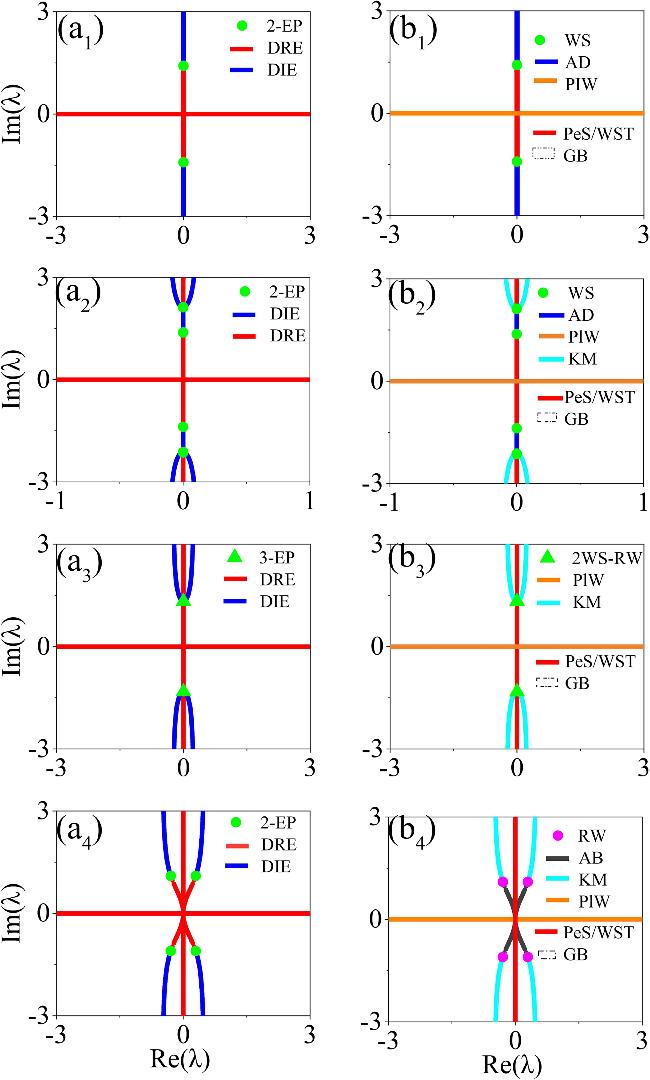
Figure 1. The left column shows the eigenvalue degeneracy patterns for a = 1. Panels a1, a2, a3, and a4 display the degeneracy regions in the ${\rm{Re}}(\lambda )-{\rm{Im}}(\lambda )$ plane for b = 0, 0.25, 0.5, and 1, respectively. Red lines, blue lines, green circles, and green triangles correspond to DRE, DIE, 2-EP, and 3-EP, respectively. Panels (b1), (b2), (b3), and (b4) show the existence regions of localized waves for b = 0, 0.25, 0.5, and 1, respectively. Gray, dark blue, light blue, red, and orange curves, as well as green circles, correspond to AB, AD, K-M, PeS/WST, PlW, and WS, respectively. Green triangles indicate the interaction of two WSs generating an RW, while blank regions correspond to GB. Magenta circles represent RW. |
For the case of zero background a = 0, the matrix U0 simplifies to a diagonal form diag(2iλ, 0, 0), with eigenvalues 2iλ, 0, and 0, as shown in figure 2. It should be noted that two eigenvalues are equal, the eigenvectors remain linearly independent, indicating the presence of non-Hermitian double degeneracy (NHDD) for the case ${\rm{Re}}(\lambda )\leqslant 0$. When ${\rm{Re}}(\lambda )=0$, converting the originally non-Hermitian Hamiltonian U0 into a Hermitian one. In this case, Hermitian double degeneracy (HDD) and Hermitian triple degeneracy (HTD) emerges, represented by the orange line and black dot, respectively, distinct from the EP in the non-Hermitian case. The corresponding eigenvectors at the HDD and HTD point maintain both completeness and orthogonality.
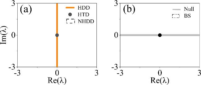
Figure 2. (a) Degeneracy regions for zero background. The white region represents non-Hermitian double degeneracy, the yellow line represents Hermitian double degeneracy, and the black dots represent Hermitian triple degeneracy. (b) Soliton existence regions. The gray lines and the blank region represent the zero solution and the bright soliton solution, respectively, and the black dots represent the soliton states in the vanishing particle number limit. |
The degeneracy of eigenvalues in linear non-Hermitian models arising from Lax-pair is well understood. The eigenvalues of the linear non-Hermitian model generate solutions (${{\rm{e}}}^{{E}_{1}}$, ${{\rm{e}}}^{{E}_{2}}$ and ${{\rm{e}}}^{{E}_{3}}$), which can be combined to form the eigenfunctions of the Lax pair. The growing and decaying solutions correspond directly to soliton solutions in the nonlinear Hermitian system. For the KM breather, the real part of the eigenvalue ${{\rm{e}}}^{{\rm{Re}}(E)\tau }$ and ${{\rm{e}}}^{{\rm{Re}}(E)\xi }$ determines both the periodicity and the width of the breather, while ${\rm{Im}}(E)=0$. In contrast, the AB breather corresponds to a purely imaginary eigenvalue, where the imaginary part of the eigenvalue ${{\rm{e}}}^{{\rm{i}}\,{\rm{Im}}(E)\tau }$ and ${{\rm{e}}}^{{\rm{i}}\,{\rm{Im}}(E)\xi }$ governs the modulation period along the evolution coordinate and the localization along the distribution coordinate. Additionally, the RW emerges as the limiting case when these two eigenvalues coalesce into a double root. At this point, the real and imaginary parts of the eigenvalue combine to form a localized structure. Moreover, by choosing different values of the spectral parameter λ, thereby constructing various types of nonlinear localized wave solutions and plane wave solutions (PWs). The existence regions of various localized wave solutions are determined by eigenvalue-dependent criteria. Then, these solution regimes can be directly mapped in the Re(λ)-Im(λ) plane. Therefore, we can analyze the corresponding relations between localized wave solutions of nonlinear Hermitian systems and eigenvalue degeneracies of linear non-Hermitian models.
The Hermitian system (1 ) supports PWs, AD, WS, KM, AB, PeS, GB, WST and RW solutions on a plane wave background. An RW and WS emerge when the two eigenvalues are equal [17, 18, 27]. An AB and a WST/PeS exist when the real parts of the eigenvalues are equal to each other [19, 27]. KM and AD when the imaginary parts of eigenvalues are equal of each other [18, 19, 27]. Based on the existence conditions determined by their eigenvalues, we present the existence regions of these solutions in the Re(λ)-Im(λ) plane in figure 1 right column. A remarkable correspondence emerges from the comparative analysis of figures 1(a) and (b): (i) the AB and WST/PeS solution domain in the nonlinear Hermitian system precisely coincides with the dispersive radiative excitation DRE regime in the non-Hermitian model (red lines); (ii) the KM and AD solution regime directly maps onto the DIE domain (blue lines); (iii) the GB solutions have no degeneracies; (iv) while RW and WS solution emerges at the 2-EPs position in the non-Hermitian framework (green dots). Particularly, the 2WS-RW solutions emerges at the 3-EPs position in the non-Hermitian framework (green triangles). When the background amplitude a = 0, the parameter space only exists BS solutions, as shows in figure 2(b). Additionally, a BS at zero density coincides with the HTD point, as marked by the black dot in figure 2(a).
The above analysis demonstrates that simple S–S equation admit significantly more abundant degeneracies in the real or imaginary spectra of linear non-Hermitian matrices than simple NLS. In particular, the multi-band Hamiltonian enables richer EP, as exemplified by the 3-EPs case shown in figure 1(a3). It allows more than two bands to coalesce at a single point, forming higher-order EPs that have attracted substantial research interest in recent years [59–61]. The Nth-order EPs can only exist in an M-state Hamiltonian when M ≥ N. As established, the scalar NLS systems admits only two eigenstates [13], by contrast, the S–S systems U0 possesses three eigenstates, enabling the realization of 3-EPs. To better visualize these EPs geometries, we treat the parameter b in the non-Hermitian Hamiltonian as an additional dimension. This approach enables construction of three-dimensional parameter-space slices, as shown in figure 3. It reveals that 2-EPs distributions constitute continuous exceptional arcs. The 2-EPs located on the imaginary axis (green curves in figure 3) correspond to the WS solutions, while other 2-EPs (rose red curves in figure 3) represent single RW solutions. The merging of two 2-EPs branches from different eigenvalues causes three eigenvalues to coincide at their intersection point, creating a 3-EP (red dots in figure 3). At a 3-EP, all three eigenvalues and their corresponding eigenvectors coalesce, reducing the rank of U0 to one and rendering it non-diagonalizable. The 3-EP lies precisely at the boundary between MI and MS. This point gives rise to two distinct WS and leads to the formation of a RW.
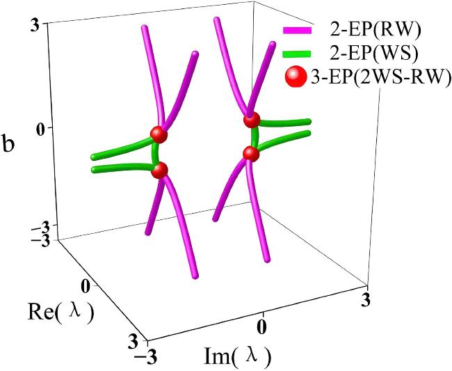
Figure 3. Distribution of EPs in the three-dimensional parameter space. The green and magenta curve represent 2-EP, the 2-EPs located on the imaginary axis (green curves) represent the WS, the other 2-EP represent the RW. The red dots represent 3-EPs, it represent the coexistence phenomenon of two WSs and an RW. |
These results demonstrate that eigenvalue degeneracies of linear non-Hermitian matrices, appearing in either the real or imaginary parts of the spectra, can serve as an efficient and quantitative descriptor of nonlinear localized-wave solutions in scalar Hermitian systems. On the other hand, the linear stability analysis around a plane wave background also leads to a non-Hermitian matrix. It is therefore natural to investigate how the degeneracy structures of these two classes of non-Hermitian matrices are related.
3. Characterizing non-Hermitian spectra of linear stability analysis
Previous works have established a direct correspondence between the spectra obtained from linear stability analysis and various families of nonlinear localized waves: the resonance line of MI corresponds to RW and KM, while the non-resonance line of MI corresponds to AB. The resonance line of MS corresponds to WS, and the non-resonance line of MI corresponds to WST [21]. In these studies, the linear stability matrix is represented by a non-Hermitian matrix. Motivated by this observation, we aim to clarify the relationship between the degeneracies of the non-Hermitian Lax-pair matrix and the matrix of linear stability analysis. In this section, we therefore begin with a linearized MI analysis on a plane wave background, derive the characteristic equation for weak perturbations, and cast it as a non-Hermitian eigenvalue problem. We consider weakly perturbed plane wave solutions of equation (3 ):
$\begin{eqnarray}q=a{{\rm{e}}}^{{\rm{i}}\theta }[1+p(x,t)],\end{eqnarray}$
where p(x, t) denotes small perturbations that expressed as superpositions of plane waves with the weakly perturbed wavenumber μk and weakly perturbed frequency μkΩk, $\begin{eqnarray}p={f}_{+}{{\rm{e}}}^{{\rm{i}}{\mu }_{k}(x+{{\rm{\Omega }}}_{k}t)}+{f}_{-}^{* }{{\rm{e}}}^{-{\rm{i}}{\mu }_{k}(x+{{\rm{\Omega }}}_{k}^{* }t)},\end{eqnarray}$
where f+ and f− denote the complex amplitudes of the perturbations. It should be noted that the perturbation wavenumber and frequency mentioned here are not the actual wavenumber and frequency of the disturbance. For a system with a plane-wave background, the actual perturbation can be expressed as aeiθp(x, t), where θ = bx + ωt with b representing the background wavenumber and ω the background frequency. Thus, the actual wavenumber and actual frequency of the perturbation are b + μk and ω + μkΩk (with ω = b3 − 6a2b), respectively. When the actual wavenumber of the perturbation equals that of the plane wave (i.e., μk = 0), the corresponding perturbation is referred to as a zero-frequency perturbation or a resonant perturbation.The instability growth rate can be defined as the imaginary part of the eigenvalue Ωk, since non-zero values of Im(Ωk) will cause exponential increase of the perturbations. Substituting weakly perturbed plane wave solutions into the KdV-type equation (equation (3 )) and ignoring the high order terms of p(x, t), we arrive at the following linear eigenvalue problem for Ωk:
$\begin{eqnarray}\begin{array}{r}{\bf{K}}\left(\begin{array}{c}{f}_{-}\\ {f}_{+}\end{array}\right)\,=\,{{\rm{\Omega }}}_{k}\left(\begin{array}{c}{f}_{-}\\ {f}_{+}\end{array}\right),\end{array}\end{eqnarray}$
with $\begin{eqnarray*}\begin{array}{rcl}{\bf{K}} & = & \left(\begin{array}{cc}{k}_{1} & {k}_{2}\\ {k}_{3} & {k}_{4}\end{array}\right),\\ {k}_{1} & = & 3{b}^{2}-3b{\mu }_{k}+{\mu }_{k}^{2}-9{a}^{2}+\frac{6{a}^{2}b}{{\mu }_{k}},\\ {k}_{2} & = & \frac{3{a}^{2}(2b-{\mu }_{k})}{{\mu }_{k}},{k}_{3}=-\frac{3{a}^{2}(2b+{\mu }_{k})}{{\mu }_{k}},\\ {k}_{4} & = & 3{b}^{2}+3b{\mu }_{k}+{\mu }_{k}^{2}-9{a}^{2}-\frac{6{a}^{2}b}{{\mu }_{k}}.\end{array}\end{eqnarray*}$
Previous studies have largely confined the analysis of MI to the matrix K, thereby establishing a correspondence between MI and the nonlinear localized waves [21]. In general K ≠ K†, indicating that K is non-Hermitian and can be regarded as an effective Hamiltonian for a non-Hermitian system, whose eigenstates satisfy the eigenvalue equation: $\begin{eqnarray}\begin{array}{r}\left(\begin{array}{cc}{k}_{1} & {k}_{2}\\ {k}_{3} & {k}_{4}\end{array}\right){\psi }_{\mu }={E}_{\mu }{\psi }_{\mu },\end{array}\end{eqnarray}$
where Eμ is the energy eigenvalues of effective Hamiltonian of a non-Hermitian system. The eigenfunction ψμ corresponds to a given set of these parameters. The energy eigenvalues are given by: $\begin{eqnarray*}\begin{array}{rcl}{E}_{\mu 1} & = & 3{b}^{2}+{\mu }_{k}^{2}-9{a}^{2}+3\sqrt{{a}^{4}+{b}^{2}({\mu }_{k}^{2}-4{a}^{2})},\\ {E}_{\mu 2} & = & 3{b}^{2}+{\mu }_{k}^{2}-9{a}^{2}-3\sqrt{{a}^{4}+{b}^{2}({\mu }_{k}^{2}-4{a}^{2})}.\end{array}\end{eqnarray*}$
The two energy branches generate three types of degeneracies: double degeneracy in the real part of eigenvalues (DREμ), double degeneracy in the imaginary part of eigenvalues (DIEμ), and double eigenvalues degeneracy. Naturally, at eigenvalues degeneracy point, the matrix K becomes non-diagonalizable, and the eigenvectors become non-orthogonal and coincide, which phenomenon is an 2-EP. Then, the degeneracy landscape can be systematically explored through variations of the background wave vector b and μk.We begin by investigating the eigenvalue degeneracies with a = 1, as illustrated in figure 4(a). The results reveal a richer degeneracy structure compared to the Lax-pair. In the b, μk parameter plane, both DREμ and DIEμ occupy open two-dimensional regions. These regions are separated by two exceptional arcs consisting of 2-EP, the two 2-EP arcs do not intersect.
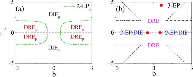


Figure 4. (a) The degeneracy of Eμ in the distribution of b and μk, with the green dashed line representing the 2-EP and the black dashed line indicating the resonance line. (b) The degeneracy of E in the distribution of b and μk. The blank regions represent parameter domains without degeneracy. The blue dashed line represents the 2-EP or DIE. The red dot denotes the 3-EP. |
The degeneracy of eigenvalues in linear non-Hermitian models arising from the linear stability analysis is well understood. The imaginary parts of the energy eigenvalues delineate MI region and the MS region [21]: when the energy eigenvalues is purely real, the system lies in the MS region; conversely, non-zero imaginary parts signal the MI region. It can be observed that a DREμ coincides with the MI region, whereas the DIEμ delineates the MS region. The interface between these regimes is set by 2-EP, which constitute the boundary in parameter space. Furthermore, the previously established correspondence between the exact localized solutions and the MI of the S–S system [21] has clearly shown that ABs correspond to the MI regime except the non-resonance line, whereas KM breathers and RWs correspond to the resonance line of MI. Meanwhile, the PeS, AD, and WST exist in the MS regime. Therefore, by combining this with the non-Hermitian spectra from the linear stability analysis shown in figure 4(a), we can conclude that AB, KM breathers, and RWs in the MI regime are all related to the DREμ, while the PeS, AD, and WST in the MS regime are all related to the DIEμ.
On the other hand, we use the soliton solutions as a bridge to map the degeneracy regions of the linear non-Hermitian models derived from the Lax pair onto the (b, μk) parameter plane, as illustrated in figure 4(b). In this representation, the resonance lines correspond to 2-EP and DIE, whereas the remaining parameter regions that still support localized wave solutions are associated with DRE. In particular, the 3-EP correspond to two distinct WS; after their collision, a RW excitation is generated [21, 62]. By comparing the degeneracy regions of these two distinct non-Hermitian matrices, as shown in figures 4(a) and (b), we find that the DREμ segments lying on the resonance lines correspond to the 2-EP or DIE regions of the linear non-Hermitian spectra, whereas the boundary between the DREμ and DIEμ regions coincides with the 3-EP.
4. Conclusion and discussion
In this work, we have established a correspondence between the nonlinear Hermitian S–S system and linear non-Hermitian models. Our results demonstrate that different types of spectral degeneracies correspond to distinct nonlinear wave structures: DRE and DIE are associated with breathers and soliton trains, NHDD corresponds to bright solitons and stationary states, 2-EP correspond to RW and WS at the transition between modulational instability and stability. However, the third-order exceptional point resides at the boundary between MI and MS, thereby establishing a unique coexistence regime between two W-shaped solitons and a rogue wave. Compared with the standard NLS equation, the S–S model exhibits a richer degeneracy structure due to its multi-band Hamiltonian, which gives rise to higher-order EP. We construct three-dimensional (Re(λ)-Im(λ)-b) parameter space slices to visualize the distribution of EPs (2-EPs and 3-EPs) for coupled systems. Furthermore, the linear stability analysis can serve as the effective Hamiltonian of a non-Hermitian system, we find that degeneracies of the real part of its spectrum coincide with the MI domain, whereas degeneracies of the imaginary part coincide with the MS domain; the two are separated by 2-EP. This offers a unifying framework linking non-Hermitian degeneracies, modulational dynamics, and nonlinear excitations. This framework can be further extended to other higher-order integrable systems, offering new insights into the interplay between linear spectral degeneracies and nonlinear localized excitations.
For non-integrable systems, the absence of a Lax pair makes it difficult to obtain exact solutions for localized waves using classical mathematical methods. As a result, one can not extend the approach used in integrable systems to directly relate nonlinear localized wave solutions to the spectral degeneracies of linear non-Hermitian systems. Fortunately, linear stability analysis remains applicable even in non-integrable systems, as the non-Hermitian coefficient matrix of the associated linear eigenvalue problem is always obtainable. Consequently, one can discuss non-Hermitian spectra of linear stability analysis within this framework. Extending it to the non-integrable S–S system, for example, our analysis shows that the MI and MS regimes correspond to the DREμ and DIEμ, respectively, with 2-EPs emerging on the critical line between them. Therefore, nonlinear excitations in these regimes can be understood by considering their non-Hermitian spectra. Thus, the framework presented here provides a viable theoretical pathway for investigating localized wave dynamics in non-integrable models through non-Hermitian spectra of linear stability analysis.