

1. Introduction
Synchronization phenomenon refers to, in the presence of coupling interaction, the alignment of the phase and frequency of two or more independently evolving systems [1]. This phenomenon was first observed and recorded by Huygens using two pendulums suspended together on the same beam in the 17th century [2]. Later, classical synchronization phenomena were extensively found in natural sciences [3] and social fields, such as a collection of fireflies [4] and neuron cells [5]. Over the past few decades, the detection and measurement of classical synchronization have been deeply studied and well-established. The measure of continuous-variable quantum synchronization proposed by Mari et al extends classical synchronization to the quantum regime [6]. The study of quantum synchronization is divided into two aspects. On the one hand, substantial efforts have focused on establishing quantitative measures for characterizing quantum synchronization [7–13]. Based on the theory of Mari et al [6], a more generalized measure referred to as quantum φ synchronization was proposed, where the relevant variables have certain phase differences [14]. Accordingly, some studies have investigated the responses of two synchronization measures to different parameters [15].
Another direction of growing interest in quantum synchronization is to search for suitable systems that exhibit quantum synchronization phenomena. Some representative research has demonstrated the possibility of observing quantum synchronization in different systems, e.g., quantum harmonic oscillators [16, 17], optomechanics [18–24], cavity and circuit quantum electrodynamics [25–27], spin [28–32] and atomic ensembles [7, 33, 34], Van der Pol (VdP) oscillators [35, 36], Bose–Einstein condensation [37] etc. Besides, by introducing an external magnon mode, nonlinear dynamics including quantum synchronization have been studied in cavity magnomechanics systems [38–42]. Among these models, optomechanical systems possess significant advantages due to the intrinsic nonlinearity of optomechanical coupling [43–47], consequently carrying the majority of the research. However, most studies focus on simple optomechanical systems with one or two coupled elements [48–51]. Meanwhile, quantum synchronization in multimode optomechanical systems has attracted considerable attention for studying information transfer and correlations between cavities and mechanical oscillators. Since multimode optomechanical systems offer more coupling configurations and facilitate complex interactions among different modes, which can be regarded as a potential platform to explore quantum correlations and other quantum effects, such as tripartite entanglement [52–55], optical nonreciprocity [56], quantum state transfer [57], phonon lasing [58, 59], ground-state cooling of oscillators [60, 61] and topological phases [62, 63]. In addition to being intensively explored in theoretical works, multimode optomechanical systems have also been experimentally demonstrated [64–70].
Inspired by this, we investigate how to achieve quantum synchronization among mechanical oscillators in a tripartite coupled optomechanical system. The system comprises three optomechanical subsystems, each with an optical cavity and a mechanical oscillator. The joint limit-cycle trajectories and Wigner functions are used to visualize the tripartite synchronization. We find that quantum synchronization and anti-synchronization [71–73] can be simultaneously achieved in a tripartite optomechanical system. Driving lasers play an important role in achieving synchronization. Accordingly, we investigate synchronization transmission by manipulating driving lasers. Moreover, we extend this configuration to a circular coupled optomechanical system and analyze the differences.
The general structure of the paper is as follows. In section 2 , we first introduce the theories of quantum synchronization, including the measures of quantum φ synchronization, quantum synchronization, and quantum anti-synchronization. In section 3.1 , we propose a coupled multimode optomechanical system, derive the quantum Langevin equations (QLEs), and obtain the time evolution of the covariance matrix. In section 3.2 , we show quantum synchronization with certain phase difference and anti-synchronization to illustrate the importance of quantum φ synchronization. Furthermore, different synchronization behaviors can simultaneously appear by applying driving lasers to three optical cavities. In section 3.3 , we use lasers to manipulate the synchronization transmission of three mechanical oscillators. In section 3.4 , we extend this model to a circular coupled optomechanical system. In section 3.5 , we compare and analyze the two different coupled multimode optomechanical systems. In section 3.6 , the impact of phonon frequency and thermal effects on quantum synchronization is studied. In section 4 , we provide the experimental implementation of the coupled optomechanical system. In section 5 , we give a conclusion and summary.
2. Measures of quantum φ synchronization, quantum synchronization and quantum anti-synchronization
In classical systems, achieving synchronization means that the error between the two systems asymptotically approaches zero after a long period of evolution. When studying quantum systems, the classical error transforms into error operators. Therefore, the degree of quantum synchronization can be quantified through the error operator. Based on previous studies, we adopt a generalized quantum φ synchronization measure [14],
$\begin{eqnarray}{S}_{\phi }=\frac{1}{\langle {q}_{-}^{\phi }{(t)}^{2}+{p}_{-}^{\phi }{(t)}^{2}\rangle },\end{eqnarray}$
the differences of variables can be characterized by defining φ error operators ${q}_{-}^{\phi }(t)=\frac{1}{\sqrt{2}}[{q}_{1}^{\phi }(t)-{q}_{2}^{\phi }(t)]$, ${p}_{-}^{\phi }(t)\,=\frac{1}{\sqrt{2}}[{p}_{1}^{\phi }(t)-{p}_{2}^{\phi }(t)]$ with $\begin{eqnarray}\begin{array}{l}{q}_{j}^{\phi }(t)={q}_{j}(t)\cos ({\phi }_{j})+{p}_{j}(t)\sin ({\phi }_{j}),\\ {p}_{j}^{\phi }(t)={p}_{j}(t)\cos ({\phi }_{j})-{q}_{j}(t)\sin ({\phi }_{j}),\end{array}\end{eqnarray}$
where qj(t) and pj(t) (j = 1, 2) are dimensionless canonical variables describing two quantum systems [6]. The phase is defined as ${\phi }_{j}=\arctan [\langle {p}_{j}(t)\rangle /\langle {q}_{j}(t)\rangle ]\,({\phi }_{j}\in [0,2\pi ])$. According to the Heisenberg uncertainty principle, the value of Sφ ranges from 0 to 1. The closer its value is to 1, the better φ synchronization can be achieved.To highlight the quantum effects on φ synchronization, the mean-field approximation is employed for the φ error operators,
$\begin{eqnarray}\begin{array}{l}{q}_{-}^{\phi }(t)\to \delta {q}_{-}^{\phi }(t)={q}_{-}^{\phi }(t)-\langle {q}_{-}^{\phi }(t)\rangle ,\\ {p}_{-}^{\phi }(t)\to \delta {p}_{-}^{\phi }(t)={p}_{-}^{\phi }(t)-\langle {p}_{-}^{\phi }(t)\rangle .\end{array}\end{eqnarray}$
When $\langle {q}_{-}^{\phi }(t)\rangle =\langle {p}_{-}^{\phi }(t)\rangle =0$, i.e., the amplitude and period of the mean values of the two variables are identical. The above quantum φ synchronization becomes $\begin{eqnarray}\begin{array}{rlr}{S}_{q}^{\phi } & =\frac{1}{\langle \delta {q}_{-}^{\phi }{(t)}^{2}+\delta {p}_{-}^{\phi }{(t)}^{2}\rangle } & \\ & =\langle \frac{1}{2}[{(\delta {p}_{1})}^{2}+{(\delta {q}_{1})}^{2}+{(\delta {p}_{2})}^{2}+{(\delta {q}_{2})}^{2}\\ & +2(\delta {p}_{1}\delta {q}_{2}-\delta {q}_{1}\delta {p}_{2})\sin \phi \\ & -2(\delta {p}_{1}\delta {p}_{2}+\delta {q}_{1}\delta {q}_{2})\cos \phi ]{\rangle }^{-1},\end{array}\end{eqnarray}$
where φ = φ2 − φ1 represents the phase difference between two oscillators. The phase difference φ is studied in two different ways: (a) mean-value synchronization with a certain phase difference is achieved with fixed parameters. The phase difference is defined as $\phi =\arctan [\langle {p}_{2}\rangle /\langle {q}_{2}\rangle ]-\arctan [\langle {p}_{1}\rangle /\langle {q}_{1}\rangle ]$, i.e., it depends on the mean values of the steady-state coordinates and momenta. Based on this, we can investigate the quantum synchronization with a phase difference φ. (b) By tuning the system parameters to achieve the mean-value synchronization with some fixed phase difference, such as φ = 0, π. Based on this, we can investigate some typical quantum synchronizations with fixed phase differences.As a generalized synchronization measure, quantum φ synchronization can describe synchronization phenomena with arbitrary phase differences. Moreover, quantum synchronization Sq and anti-synchronization ${\widetilde{S}}_{q}$ are the special cases of quantum φ synchronization for φ = 0(π). When φ = 0, quantum φ synchronization ${S}_{q}^{\phi }$ is completely equivalent to quantum synchronization Sq proposed by Mari et al [6],
$\begin{eqnarray}{S}_{q}=\frac{1}{\langle \delta {q}_{-}{(t)}^{2}+\delta {p}_{-}{(t)}^{2}\rangle },\end{eqnarray}$
which can be regarded as a special case of quantum φ synchronization. The measure of quantum synchronization needs to satisfy the condition of complete mean-value synchronization. Therefore, the mean-value synchronization is treated as the first-order measure to assess whether the average trajectories of mechanical oscillators are synchronized [45]. Quantum synchronization measure can be regarded as the second-order synchronization measure to reflect the differences of quantum fluctuations between two quantum systems.Another special case is when φ = π, quantum φ synchronization ${S}_{q}^{\phi }$ becomes quantum anti-synchronization ${\widetilde{S}}_{q}$ [14]. Hence, we can employ ${\widetilde{S}}_{q}$ to quantify quantum anti-synchronization,
$\begin{eqnarray}\begin{array}{l}{\widetilde{S}}_{q}\equiv {S}_{q}^{\pi }=\frac{1}{\langle \delta {q}_{-}^{\pi }{(t)}^{2}+\delta {p}_{-}^{\pi }{(t)}^{2}\rangle }\\ \quad ={\left\langle \frac{1}{2}[{(\delta {q}_{1}+\delta {q}_{2})}^{2}+{(\delta {p}_{1}+\delta {p}_{2})}^{2}]\right\rangle }^{-1}.\end{array}\end{eqnarray}$
The mean-value anti-synchronization serves as a prerequisite for quantum anti-synchronization. The mean-value anti-synchronization can be observed by the average trajectories of mechanical oscillators, and quantum anti-synchronization can be calculated by the measure of ${\widetilde{S}}_{q}$.In summary, quantum φ synchronization is more generalized and reasonable in measuring quantum synchronization. It removes mean-value synchronization as a prerequisite and enables the measurement of the changes in phase difference with different parameters.
3. Synchronization transmission in a multimode coupled optomechanical system
3.1. The model and dynamics of the optomechanical system
We consider a coupled multimode optomechanical system comprised of three optical cavities, and each has a mechanical oscillator with different frequencies [74] [see figure 1]. Two cavities a1 and a3 are indirectly coupled via the intermediate detuned cavity a2 [75]. The coupling between the nearest cavities can be mediated by optical fibers [76]. The Hamiltonian of the system can be written as (ℏ = 1),
$\begin{eqnarray}\begin{array}{rcl}H & = & \displaystyle \sum _{j=1}^{3}{H}_{mj}+{H}_{d}+{H}_{I},\\ {H}_{mj} & = & \left\{\Space{0ex}{2.25ex}{0ex}-{{\rm{\Delta }}}_{j}[1+{\eta }_{c}\cos ({{\rm{\Omega }}}_{c}t)]{a}_{j}^{\dagger }{a}_{j}\right.\\ & & \left.+\frac{{\omega }_{j}}{2}({p}_{j}^{2}+{q}_{j}^{2})-g{a}_{j}^{\dagger }{a}_{j}{q}_{j}\right\},\\ {H}_{d} & = & {\rm{i}}E({a}_{1}^{\dagger }-{a}_{1})+{\rm{i}}E({a}_{3}^{\dagger }-{a}_{3}),\\ {H}_{I} & = & {\lambda }_{1}({a}_{1}^{\dagger }{a}_{2}+{a}_{2}^{\dagger }{a}_{1})+{\lambda }_{2}({a}_{2}^{\dagger }{a}_{3}+{a}_{3}^{\dagger }{a}_{2}),\end{array}\end{eqnarray}$
where aj is the dimensionless annihilation field operator of the jth optical cavity with frequency ωcj, and it satisfies the canonical commutation relation $[{a}_{j},{a}_{j}^{\dagger }]=1$. qj and pj describe the dimensionless position and momentum operators of the jth mechanical oscillator and satisfy the canonical commutation relation $[{q}_{j},{p}_{{j}^{{\prime} }}]={\rm{i}}{\delta }_{j{j}^{{\prime} }}$. ωj represents the different frequencies of the three mechanical oscillators [77, 78]. We assume each mechanical oscillator is coupled to its optical cavity through radiation pressure with the same strength g [79]. λj is the coupling interaction between the nearest cavities [80, 81]. The optical cavities at both ends are driven by the same pump laser beam with frequency ωL and intensity E. Δj = ωcj − ωL represents the cavity detuning. According to the current study [82–84], we exert periodic modulation with frequency Ωc and amplitude ηc on the cavity detuning to enhance quantum synchronization and achieve different synchronization phenomena [85–91].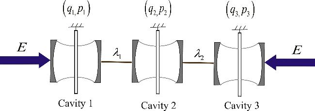
Figure 1. Schematic illustration of the three coupled cavity optomechanical systems. Each consists of a mechanical oscillator with different frequencies coupled via radiation pressure to an optical cavity aj (j = 1, 2, 3). The three optical cavities are directly coupled with their nearest neighbor via a coupling constant λj. E is the laser driving strength. |
We consider the fluctuation-dissipation effects and derive the quantum Langevin equations (QLEs) from the above Hamiltonian for cavities and mechanical oscillators [43, 92–94]. Hence, the time evolution of the relevant operators of the optomechanical system aj, qj, and pj (j = 1, 2, 3) can be given by,
$\begin{eqnarray}\begin{array}{rcl}\dot{{q}_{j}} & = & {\omega }_{j}{p}_{j},\\ \dot{{p}_{j}} & = & -{\omega }_{j}{q}_{j}-\gamma {p}_{j}+g{a}_{j}^{\dagger }{a}_{j}+{\xi }_{j},\\ \dot{{a}_{1}} & = & -\left\{\kappa -{\rm{i}}{{\rm{\Delta }}}_{1}\left[1+{\eta }_{c}\cos ({{\rm{\Omega }}}_{c}t)\right]\right\}{a}_{1}\\ & & +{\rm{i}}g{a}_{1}{q}_{1}+E-{\rm{i}}{\lambda }_{1}{a}_{2}+\sqrt{2\kappa }{a}_{1}^{{\rm{in}}},\\ \dot{{a}_{2}} & = & -\left\{\kappa -{\rm{i}}{{\rm{\Delta }}}_{2}\left[1+{\eta }_{c}\cos ({{\rm{\Omega }}}_{c}t)\right]\right\}{a}_{2}\\ & & +{\rm{i}}g{a}_{2}{q}_{2}-{\rm{i}}{\lambda }_{1}{a}_{1}-{\rm{i}}{\lambda }_{2}{a}_{3}+\sqrt{2\kappa }{a}_{2}^{{\rm{in}}},\\ \dot{{a}_{3}} & = & -\left\{\kappa -{\rm{i}}{{\rm{\Delta }}}_{3}\left[1+{\eta }_{c}\cos ({{\rm{\Omega }}}_{c}t)\right]\right\}{a}_{3}\\ & & +{\rm{i}}g{a}_{3}{q}_{3}+E-{\rm{i}}{\lambda }_{2}{a}_{2}+\sqrt{2\kappa }{a}_{3}^{{\rm{in}}},\end{array}\end{eqnarray}$
where κ and γ are the decay rates of the optical cavities and mechanical oscillators, respectively [95, 96]. ${a}_{j}^{{\rm{in}}}$ denotes the vacuum optical noise and satisfy the correlation function $\left\langle {a}_{j}^{{\rm{in}}\dagger }(t){a}_{{j}^{{\prime} }}^{{\rm{in}}}({t}^{{\prime} })+{a}_{{j}^{{\prime} }}^{{\rm{in}}}({t}^{{\prime} }){a}_{j}^{{\rm{in}}\dagger }(t)\right\rangle ={\delta }_{j{j}^{{\prime} }}\delta (t-{t}^{{\prime} })$ under a zero-temperature assumption [97]. ξj denotes the Brownian noise operator of the mechanical oscillators, which satisfies $\frac{1}{2}\langle {\xi }_{j}(t){\xi }_{{j}^{{\prime} }}({t}^{{\prime} })+{\xi }_{{j}^{{\prime} }}({t}^{{\prime} }){\xi }_{j}(t)\rangle =\gamma (2{\bar{n}}_{{\rm{bath}}}+1){\delta }_{j{j}^{{\prime} }}\delta (t-{t}^{{\prime} })$. ${\bar{n}}_{{\rm{bath}}}\,=1/[\exp \left(\hslash {\omega }_{j}/{k}_{{\rm{B}}}T\right)-1]$ is the mean thermal phonon number at temperature T and kB is the Boltzmann constant [98, 99].In the limit of large photon number, we can follow the standard mean-field approximation [100], whereby the operators can be divided into mean values and fluctuation terms, 9 ) into equation (8 ), the mean-value equations can be written as, 11 ) can be expressed as,
$\begin{eqnarray}{a}_{j}(t)={\alpha }_{j}(t)+\delta {a}_{j}(t),\,{O}_{j}(t)={\bar{O}}_{j}(t)+\delta {O}_{j}.\,(O=q,p).\end{eqnarray}$
The mean-value of the given operators can be treated as classical variables, and the quantum properties of the system can be reflected by the fluctuation terms. By substituting equation ( $\begin{eqnarray}\begin{array}{rcl}{\dot{\bar{q}}}_{j} & = & {\omega }_{j}{\bar{p}}_{j},\\ {\dot{\bar{p}}}_{j} & = & -{\omega }_{j}{\bar{q}}_{j}-\gamma {\bar{p}}_{j}+g| {\alpha }_{j}{| }^{2},\\ \dot{{\alpha }_{1}} & = & -\left\{\kappa -{\rm{i}}{{\rm{\Delta }}}_{1}\left[1+{\eta }_{c}\cos ({{\rm{\Omega }}}_{c}t)\right]\right\}{\alpha }_{1}\\ & & +{\rm{i}}g{\alpha }_{1}{\bar{q}}_{1}+E-{\rm{i}}{\lambda }_{1}{\alpha }_{2},\\ \dot{{\alpha }_{2}} & = & -\left\{\kappa -{\rm{i}}{{\rm{\Delta }}}_{2}\left[1+{\eta }_{c}\cos ({{\rm{\Omega }}}_{c}t)\right]\right\}{\alpha }_{2}\\ & & +{\rm{i}}g{\alpha }_{2}{\bar{q}}_{2}-{\rm{i}}{\lambda }_{1}{\alpha }_{1}-{\rm{i}}{\lambda }_{2}{\alpha }_{3},\\ \dot{{\alpha }_{3}} & = & -\left\{\kappa -{\rm{i}}{{\rm{\Delta }}}_{3}\left[1+{\eta }_{c}\cos ({{\rm{\Omega }}}_{c}t)\right]\right\}{\alpha }_{3}\\ & & +{\rm{i}}g{\alpha }_{3}{\bar{q}}_{3}+E-{\rm{i}}{\lambda }_{2}{\alpha }_{2},\end{array}\end{eqnarray}$
and the linear equations for quantum fluctuations are given by, $\begin{eqnarray}\begin{array}{rcl}\delta {\dot{q}}_{j} & = & {\omega }_{j}\delta {p}_{j},\\ \delta {\dot{p}}_{j} & = & -{\omega }_{j}\delta {q}_{j}-\gamma \delta {p}_{j}+g({\alpha }_{j}\delta {a}_{j}^{\dagger }+{\alpha }_{j}^{* }\delta {a}_{j})+{\xi }_{j},\\ \delta \dot{{a}_{1}} & = & -\left\{\kappa -{\rm{i}}{{\rm{\Delta }}}_{1}\left[1+{\eta }_{c}\cos ({{\rm{\Omega }}}_{c}t)\right]\right\}\delta {a}_{1}\\ & & +{\rm{i}}g({\alpha }_{1}\delta {q}_{1}+{\bar{q}}_{1}\delta {a}_{1})-{\rm{i}}{\lambda }_{1}\delta {a}_{2}+\sqrt{2\kappa }{a}_{1}^{{\rm{in}}},\\ \delta \dot{{a}_{2}} & = & -\left\{\kappa -{\rm{i}}{{\rm{\Delta }}}_{2}\left[1+{\eta }_{c}\cos ({{\rm{\Omega }}}_{c}t)\right]\right\}\delta {a}_{2}\\ & & +{\rm{i}}g({\alpha }_{2}\delta {q}_{2}+{\bar{q}}_{2}\delta {a}_{2})-{\rm{i}}{\lambda }_{1}\delta {a}_{1}-{\rm{i}}{\lambda }_{2}\delta {a}_{3}+\sqrt{2\kappa }{a}_{2}^{{\rm{in}}},\\ \delta \dot{{a}_{3}} & = & -\left\{\kappa -{\rm{i}}{{\rm{\Delta }}}_{3}\left[1+{\eta }_{c}\cos ({{\rm{\Omega }}}_{c}t)\right]\right\}\delta {a}_{3}\\ & & +{\rm{i}}g({\alpha }_{3}\delta {q}_{3}+{\bar{q}}_{3}\delta {a}_{3})-{\rm{i}}{\lambda }_{2}\delta {a}_{2}+\sqrt{2\kappa }{a}_{3}^{{\rm{in}}},\end{array}\end{eqnarray}$
the second-order terms of quantum fluctuation equations are ignored. Then we introduce the optical field transformation $\delta {x}_{j}=\frac{1}{\sqrt{2}}\left(\delta {a}_{j}+\delta {a}_{j}^{\dagger }\right),\delta {y}_{j}=\frac{1}{\sqrt{2}{\rm{i}}}\left(\delta {a}_{j}-\delta {a}_{j}^{\dagger }\right)$. Therefore, the linear quantum fluctuation equation ( $\begin{eqnarray}\dot{u}(t)=M(t)u(t)+n(t),\end{eqnarray}$
where the column vector can be defined as $u(t)={({h}_{1},{h}_{2},{h}_{3})}^{\top }$, with hj = (δqj, δpj, δxj, δyj). The corresponding noise column vector is $n(t)={({h}_{1}^{{\rm{in}}},{h}_{2}^{{\rm{in}}},{h}_{3}^{{\rm{in}}})}^{\top }$, with ${h}_{j}^{{\rm{in}}}=(0,{\xi }_{j},\sqrt{2\kappa }{x}_{j}^{{\rm{in}}},\sqrt{2\kappa }{y}_{j}^{{\rm{in}}})$ as well as ${x}_{j}^{{\rm{in}}}=\frac{1}{\sqrt{2}}\left({a}_{j}^{{\rm{in}}}+{a}_{j}^{{{\rm{in}}}^{\dagger }}\right)$, ${y}_{j}^{{\rm{in}}}\,=\frac{1}{\sqrt{2}{\rm{i}}}\left({a}_{j}^{{\rm{in}}}-{a}_{j}^{{{\rm{in}}}^{\dagger }}\right)$. M(t) can be written as a time-dependent matrix, $\begin{eqnarray}M(t)=\left(\begin{array}{ccc}{B}_{1} & {D}_{1} & 0\\ {D}_{1} & {B}_{2} & {D}_{2}\\ 0 & {D}_{2} & {B}_{3}\\ \end{array}\right),\end{eqnarray}$
where Bj (j = 1, 2, 3) and Dj are 4 × 4 matrices. The sub-block Bj is written as follows $\begin{eqnarray}{B}_{j}=\left(\begin{array}{cccc}0 & {\omega }_{j} & 0 & 0\\ -{\omega }_{j} & -\gamma & \sqrt{2}g{\rm{Re}}({\alpha }_{j}) & \sqrt{2}g{\rm{Im}}({\alpha }_{j})\\ -\sqrt{2}g{\rm{Im}}({\alpha }_{j}) & 0 & -\kappa & -{A}_{j}\\ \sqrt{2}g{\rm{Re}}({\alpha }_{j}) & 0 & {A}_{j} & -\kappa \end{array}\right),\end{eqnarray}$
with ${A}_{j}={{\rm{\Delta }}}_{j}[1+{\eta }_{c}\cos ({{\rm{\Omega }}}_{c}t)]+g{\bar{q}}_{j}$, ${\rm{Re}}({\alpha }_{j})$ and ${\rm{Im}}({\alpha }_{j})$ are the real and imaginary parts of the mean-value of the cavity.Dj represents the interaction between each pair of cavities, which can be written as10 ). The quantum characteristic of the optomechanical system can be governed by the linear Langevin equations containing fluctuation operators. To study the properties of quantum synchronization, it is necessary to define a 12 × 12 covariance matrix Vkl, which can completely reflect the Gaussian state properties. Moreover, each element of the covariance matrix Vkl can be extracted as follows12 ) and (16 ), the time evolution of V(t) can be rewritten as [100–102],
$\begin{eqnarray}{D}_{j}=\left(\begin{array}{cccc}0 & 0 & 0 & 0\\ 0 & 0 & 0 & 0\\ 0 & 0 & 0 & {\lambda }_{j}\\ 0 & 0 & -{\lambda }_{j} & 0\end{array}\right).\end{eqnarray}$
The solution of the matrix M(t) can be obtained by numerically solving equation ( $\begin{eqnarray}{V}_{kl}\equiv \frac{1}{2}\langle {u}_{k}{u}_{l}+{u}_{l}{u}_{k}\rangle .\end{eqnarray}$
The degree of quantum synchronization can be calculated by using the elements of the covariance matrix Vkl. It is convenient to utilize different quantum synchronization measures Sq, ${\widetilde{S}}_{q}$ and ${S}_{q}^{\phi }$ to quantify the synchronization of two mechanical oscillators. We only rewrite the synchronization measures of the first two mechanical oscillators, $\begin{eqnarray}\begin{array}{rcl}{S}_{{q}_{12}} & = & {\left[\frac{1}{2}({V}_{11}+{V}_{22}+{V}_{55}+{V}_{66}-{V}_{15}-{V}_{51}-{V}_{26}-{V}_{62})\right]}^{-1},\\ {\widetilde{S}}_{{q}_{12}} & = & {\left[\frac{1}{2}({V}_{11}+{V}_{22}+{V}_{55}+{V}_{66}+{V}_{15}+{V}_{51}+{V}_{26}+{V}_{62})\right]}^{-1},\\ {S}_{{q}_{12}}^{\phi } & = & \left[\frac{1}{2}({V}_{11}+{V}_{22}+{V}_{55}+{V}_{66}+2{V}_{25}\sin \phi \right.\\ & & {\left.-2{V}_{16}\sin \phi -2{V}_{15}\cos \phi -2{V}_{26}\cos \phi )\right]}^{-1},\end{array}\end{eqnarray}$
the form of the synchronization measures for the other two pairs ${S}_{{q}_{13}}$ and ${S}_{{q}_{23}}$ remains invariant, only exchanging the subscript kl. In addition, the time-averaged synchronization measure is redefined as ${\bar{S}}_{q}^{(\phi )}=\mathop{\mathrm{lim}}\limits_{T\to \infty }\frac{1}{T}{\int }_{0}^{T}{S}_{q}^{(\phi )}(t){\rm{d}}t$ in the asymptotic steady state of the system. From Equations ( $\begin{eqnarray}\dot{V}(t)=M(t)V(t)+V(t)M{(t)}^{T}+N,\end{eqnarray}$
where N = diag[C1, C2, C3] is the diagonal noise matrix with ${C}_{j}={\rm{diag}}[0,\gamma (2{\bar{n}}_{{\rm{bath}}}+1),\kappa ,\kappa ]$, satisfying ${N}_{ij}\delta (t-{t}^{{\prime} })\,=\frac{1}{2}\langle {\hat{\xi }}_{i}(t){\hat{\xi }}_{j}({t}^{{\prime} })+{\hat{\xi }}_{j}({t}^{{\prime} }){\hat{\xi }}_{i}(t)\rangle $.The prerequisite for studying quantum synchronization is to ensure that all eigenvalues of the coefficient matrix M(t) are negative after transient evolution, as determined by the Routh–Hurwitz criterion [103]. At this time, the stability conditions of the optomechanical system can be assured. Consequently, the system evolves into a steady state where the variables of oscillators show limit-cycle synchronization [104]. The parameters are selected to satisfy the stability conditions. In addition, the system parameters also need to meet the following conditions to achieve stability [105], $\begin{eqnarray}\begin{array}{l}2\gamma \kappa [{{\rm{\Delta }}}^{4}+{{\rm{\Delta }}}^{2}({\gamma }^{2}+2\gamma \kappa +2{\kappa }^{2}-2{\omega }_{j}^{2})\\ \quad +\,{(\gamma \kappa +{\kappa }^{2}+{\omega }_{j}^{2})}^{2}]+{\omega }_{j}{G}_{j}^{2}{\rm{\Delta }}{(\gamma +2\kappa )}^{2}\,\gt \,0,\\ \quad {\omega }_{j}^{2}({{\rm{\Delta }}}^{2}+{\kappa }^{2})-{\omega }_{j}{G}_{j}^{2}{\rm{\Delta }}\,\gt \,0,\end{array}\end{eqnarray}$
where, ${G}_{j}\equiv \sqrt{2}g{\alpha }_{j}$ is defined as effective coupling constant. By choosing the phase reference of the cavity mode, αj can be considered to be real.In addition, quantum synchronization can be visualized by the single mode Gaussian Wigner function in phase space [106],
$\begin{eqnarray}\begin{array}{r}W(R)=\frac{1}{\pi \sqrt{{\rm{\det }}[\sigma ]}}{\rm{\exp }}\left(-\frac{1}{2}(R-{\bar{R)}}^{\top }{\sigma }^{-1}(R-\bar{R)}\right),\end{array}\end{eqnarray}$
where R = [q, p]⊤ is the quadrature operator of the oscillator. $\bar{R}={[\langle q\rangle ,\langle p\rangle ]}^{\top }$ is the displacement column vector. The covariance matrix is defined as σjk =⟨{Rj, Rk}⟩/2 − ⟨Rj⟩⟨Rk⟩. Tripartite quantum synchronization can be more effectively manifested through the Wigner functions.3.2. Quantum synchronization of next-nearest-neighboring mechanical oscillators
As we know, quantum synchronization can occur between two coupled systems. Under these circumstances, two independent subsystems cannot synchronize, and connecting an additional cavity can facilitate synchronization. Therefore, we will explore how to achieve quantum synchronization in a multimode coupled optomechanical system and exhibit different synchronization behaviors. By driving optical cavities at both ends, we investigate the behaviors of quantum synchronization between oscillator 1 and oscillator 3 via an intermediate detuned cavity a2. The parameter selections are similar to Mari's work [6] and some current studies [14, 15, 44, 45, 71, 86, 87, 107, 108]. Moreover, these parameters are feasible for experimental implementation. In the rest of the paper, we take Δ1 = 1 as a reference unit, and all the parameters are evaluated in units of Δ1. In the numerical simulations, we set the initial conditions of each subsystem to zero. As shown in figure 2(a), the mean-value of position $({\bar{q}}_{1},{\bar{q}}_{3})$ and momentum $({\bar{p}}_{1},{\bar{p}}_{3})$ of mechanical oscillators can reach a limit-cycle trajectory in classical phase space. This implies that the system can reach a steady state, which establishes the prerequisite for studying quantum synchronization. As shown in figures 2(c) and (d), two mechanical oscillators can achieve synchronization by coherent information transfer among the different cavities, and the phase difference is φ = 0.5π. In this scenario, the quantum synchronization measure Sq is no longer applicable. Thus, for coupled mechanical oscillators with non-zero φ, we need to employ quantum φ synchronization ${S}_{q}^{\phi }$ to measure synchronization between two mechanical oscillators in figure 2(b).
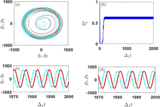
Figure 2. (a) The evolution of the mean values ${\bar{q}}_{1},{\bar{q}}_{3}$ and ${\bar{p}}_{1},{\bar{p}}_{3}$ (dimensionless variables) of the two mechanical oscillators' position and momentum (blue and red lines), (b) time evolution of quantum φ synchronization ${S}_{q}^{\phi }(t)$, (c) time evolution of the mean values ${\bar{q}}_{1}(t)$ (red solid line) and ${\bar{q}}_{3}(t)$ (cyan dashed line), (d) time evolution of the mean values ${\bar{p}}_{1}(t)$ (red solid line) and ${\bar{p}}_{3}(t)$ (cyan dashed line). The other parameters used in the simulation are ω1 = Δ1, ω2 = 1.01Δ1, ω3 = 1.005Δ1, ηc = 3Δ1, Ωc = 4Δ1, Δ1 = ω1, Δ2 = ω2, Δ3 = ω3, E = 100Δ1, λ1 = λ2 = 0.03Δ1, g = 0.005Δ1, k = 0.15Δ1, γ = 0.005Δ1${\bar{n}}_{{\rm{bath}}}=0$. |
Moreover, by adjusting the periodic modulation and coupling interaction between the adjacent cavities, we find quantum anti-synchronization between the next-nearest-neighboring mechanical oscillators. Figure 3(a) shows the stable limit-cycle trajectories of two mechanical oscillators in phase space, indicating that the oscillators exhibit periodic oscillation behavior. As shown in figures 3(c) and (d), the time evolutions of ${\bar{q}}_{1}({\bar{p}}_{1})$ and ${\bar{q}}_{3}({\bar{p}}_{3})$ evolve out of phase from each other with similar vibrational amplitudes. It indicates that the mean-value of mechanical oscillators can achieve anti-synchronization. An important point is to assess quantum anti-synchronization, we can utilize equation (6 ) to quantify ${\widetilde{S}}_{q}$ in figure 3(b). In this scenario, not only can mean-value anti-synchronization be achieved, but quantum anti-synchronization can also be observed.
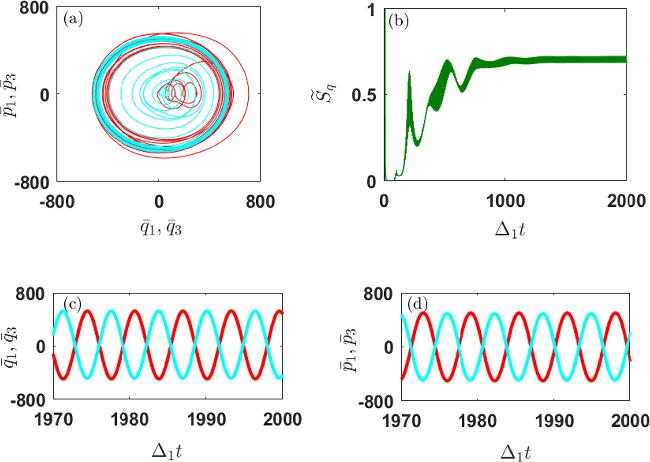
Figure 3. (a) The evolution of the mean values ${\bar{q}}_{1},{\bar{q}}_{3}$ and ${\bar{p}}_{1},{\bar{p}}_{3}$ (dimensionless variables) of the two mechanical oscillators' position and momentum (red and cyan lines), (b) time evolution of quantum anti-synchronization ${\widetilde{S}}_{q}(t)$, (c) time evolution of the mean values ${\bar{q}}_{1}(t)$ (red solid line) and ${\bar{q}}_{3}(t)$ (cyan solid line), (d) time evolution of the mean values ${\bar{p}}_{1}(t)$ (red solid line) and ${\bar{p}}_{3}(t)$ (cyan solid line). Here, we set ηc = 2Δ1, Ωc = 2Δ1, λ1 = 0.3Δ1, λ2 = 0.2Δ1. Other parameters are the same as in figure 2. |
In the scenarios above, quantum synchronization between mechanical oscillators 1 and 3 can be achieved via coherent information transfer among different optical cavities. The middle cavity a2 serves as a connecting link and the setting of the driving field for it is absent. The behaviors of its mechanical oscillator are neglected due to the lack of complete quantum synchronization with the other two oscillators. This demonstrates that in optomechanical systems, an effective driving laser is essential for observing quantum synchronization phenomena.
To achieve synchronization between each pair of mechanical oscillators, an external driving field E = 100Δ1 is applied to the intermediate cavity a2. We study the quantum synchronization behaviors between any two mechanical oscillators in this configuration, which is termed a linear coupled optomechanical system. The cavities a1 and a3 are detuned from the intermediate cavity a2, respectively. We examine the stability of the system, and synchronization occurs based on the limit-cycle steady state. As shown in figure 4(a), the joint limit-cycle trajectories of three mechanical oscillators are plotted, which can be used to visualize mean-value synchronization for the tripartite systems. The evolutions of ⟨q1⟩⇌⟨p1⟩ (red line), ⟨q2⟩⇌⟨p2⟩ (blue line) and ⟨q3⟩⇌⟨p3⟩ (cyan line) tend to a consistent orbit in phase space. It means that the mean-field trajectories of the three mechanical oscillators exhibit perfect synchronization. Moreover, two types of quantum synchronization behaviors are simultaneously exhibited in the optomechanical system. As shown in figures 4(b) and (c), the mean values of oscillators 1 and 2 exhibit anti-synchronize with opposite amplitude. Moreover, the measure ${\widetilde{S}}_{q}$ can also reflect that synchronization behaviors still exist in the quantum regime in figure 4(d). The same phenomena are also observed between the oscillators 2 and 3 in figures 4(h) and (i). Since any adjacent mechanical oscillators vibrate with opposite amplitudes, the next-nearest mechanical oscillators 1 and 3 naturally achieve complete quantum synchronization with equal amplitudes in figures 4 (e) and (f). The evolutions of ${\bar{q}}_{1}({\bar{p}}_{1})$ and ${\bar{q}}_{3}({\bar{p}}_{3})$ are accordant with phase difference φ = 0. Therefore, quantum synchronization Sq can serve as a normative measure to quantify the degree of synchronization in figure 4(g). While the mean values can achieve complete synchronization, quantum fluctuations may still exhibit differences. This explains why the degree of quantum synchronization Sq remains below unity. Figure 5 displays the Gaussian Wigner functions of three mechanical modes. It can be shown that three mechanical oscillators form a ring structure in quantum phase space, which provides a direct visualization of the quantum synchronization phenomenon between these systems.
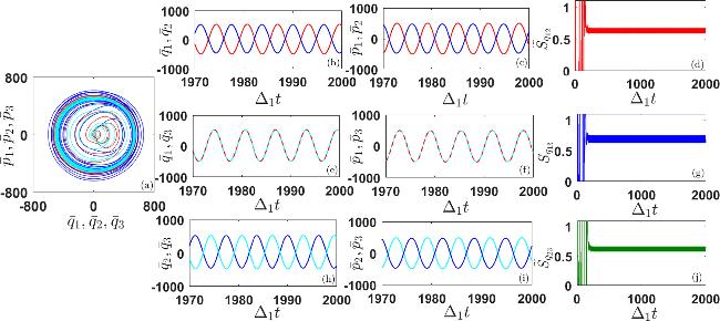
Figure 4. (a) The joint limit-cycle trajectories of the oscillators. The evolution of the (b) mean values of ${\bar{q}}_{1}(t)$ (red line), ${\bar{q}}_{2}(t)$ (blue line), (c) mean values of ${\bar{p}}_{1}(t)$ (red line), ${\bar{p}}_{2}(t)$ (blue line), (d) quantum anti-synchronization ${\widetilde{S}}_{{q}_{12}}(t)$. (e) Mean values of ${\bar{q}}_{1}(t)$ (red line), ${\bar{q}}_{3}(t)$ (cyan dashed line), (f) mean values of ${\bar{p}}_{1}(t)$ (red line), ${\bar{p}}_{3}(t)$ (cyan dashed line), (g) quantum synchronization ${S}_{{q}_{13}}(t)$. (h) Mean values of ${\bar{q}}_{2}(t)$ (blue line), ${\bar{q}}_{3}(t)$ (cyan line), (i) mean values of ${\bar{p}}_{2}(t)$ (blue line), ${\bar{p}}_{3}(t)$ (cyan line), (j) quantum anti-synchronization ${\widetilde{S}}_{{q}_{23}}(t)$. Here, we set three cavities to be driven by lasers with intensity E = 100Δ1. Other parameters are the same in figure 2. |
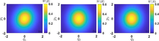
Figure 5. Wigner functions of the three mechanical oscillators. The mean values of the mechanical oscillator's position and momentum are shifted to the origin. The parameter settings are the same as in figure 4. |
In addition, we show the synchronization phase diagram characterized by Sq to study the effects of parameters on achieving quantum synchronization in multimode coupled optomechanical systems. The synchronization phase diagram in the E − λj plane is shown in figure 6(a). When the driving strength E is in the range of 60Δ1 to 120Δ1, the value of Sq is approximately 0.9, indicating that a good quantum synchronization can be achieved. Therefore, we can set E = 100Δ1 in the simulation to achieve optimal synchronization. When the driving intensity E is locked within this range, the coupling interaction between cavities can vary within a wide range without affecting the quantum synchronization behaviors. However, once E > 120Δ1, synchronization becomes unstable accompanied by a decrease in the synchronization measure Sq. As shown in figure 6(b), quantum synchronization in the ηc − g plane exhibits a similar trend. When the modulation amplitude of the optical cavity ηc is in the range of 2Δ1 to 5Δ1 and optomechanical coupling g is maintained below 5.5 × 10⁻³Δ1, good quantum synchronization behaviors can be achieved. Based on this, we can find a certain parameter range to achieve good quantum synchronization behavior. Therefore, the parameters selected from this range can optimize quantum synchronization effects.
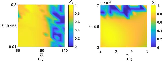
Figure 6. Synchronization phase diagram in terms of quantum synchronization measure Sq in the (a) E − λj plane under ηc = 2.5Δ1, ωc = 3Δ1. (b) ηc − g plane. Other parameters are the same in figure 2. |
3.3. Synchronization transmission of three mechanical oscillators
Our previous analysis shows that driving lasers are essential for achieving synchronization, and thus lasers can be used to manipulate and control synchronization transmission among mechanical oscillators. By modulating the driving lasers, the optical cavities have correlations and the mechanical oscillators in these cavities can achieve quantum synchronization. In addition to theoretical explanations, relevant experimental studies have also been carried out. Some studies have demonstrated that synchronization of silicon nitride micromechanical oscillator arrays can be manipulated and achieved by adjusting the laser power [109]. When driving lasers are coupled to optical cavities spanning multiple mechanical oscillators, the laser not only ensures that the mechanical oscillators achieve self-sustaining oscillations but also provides the necessary optomechanical coupling for synchronization. When the laser power is high enough to overcome the natural frequency of the mechanical oscillators, the mechanical oscillators can achieve synchronization. As the laser power increases, quantum synchronization can be extended and transferred from three coupled optomechanical systems to four, and even further to seven coupled optomechanical systems. In other words, the number of synchronized coupled optomechanical systems can be manipulated by adjusting the laser parameters. Furthermore, synchronization can also be experimentally achieved based on long-distance optomechanical coupling by tuning the frequency of laser driving [70]. In addition, some experiments have demonstrated that synchronization effects can be achieved by using an input laser in two mechanically coupled optomechanical cells in an optomechanical array [110]. Therefore, the quantum synchronization phenomenon of adjacent or next-nearest-neighbor mechanical oscillators and synchronization transfer in optomechanical arrays are experimentally studied by tuning the driving laser.
Under the effects of driving lasers, optical cavities can exhibit correlations and enable coherent information transfer, which facilitates quantum synchronization and synchronization transfer between mechanical oscillators. As shown in figure 7(a), we first apply driving lasers to cavities 1 and 2. Due to the influence of the driving fields and coherent information transfer among optical cavities, the mechanical oscillators in these cavities can achieve synchronization. In order to transfer synchronization from oscillators 1 and 2 to oscillators 2 and 3, the laser is applied to cavity 3, i.e., cavities 2 and 3 are now driven instead [see figure 7(b)]. Overall, we can use lasers to control the synchronization of mechanical oscillators and realize synchronization transfer between adjacent mechanical oscillators. Based on this, we can extend the model to optomechanical chains [see figure 7(c)]. It is anticipated that the quantum synchronization of adjacent mechanical oscillators can be controlled step-by-step via driving lasers. Moreover, we can also achieve synchronization of multiple mechanical oscillators by increasing the number of laser drives and adjusting the laser parameters. Therefore, driving lasers have a significant impact on quantum synchronization transmission among mechanical oscillators in a coupled multimode optomechanical system.
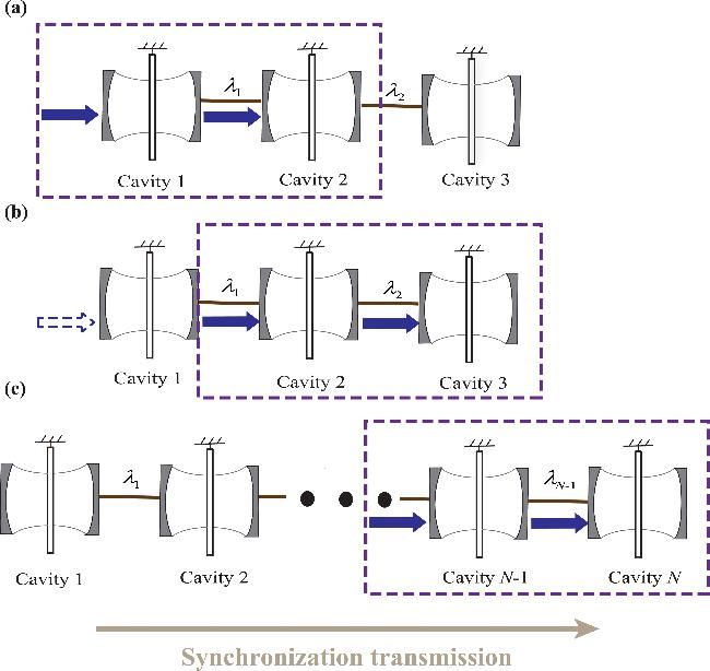
Figure 7. Schematic illustration of mechanical oscillators synchronous transmission manipulated by driving laser in coupled multimode optomechanical systems. (a) Driving lasers are applied to the cavities 1 and 2. (b) Driving lasers are applied to the cavities 2 and 3. (c) The step-by-step control of multiple mechanical oscillators synchronization using lasers in the optomechanical chain. |
3.4. Quantum synchronization in a circular coupled optomechanical system
Now we consider a circular coupled optomechanical system where the external direct coupling interaction between cavities a1 and a3 is taken into account. For simplicity, we set the coupling interactions are the same in our proposed optomechanical system, i.e., λ1 = λ2 = λ3 = λ. The Hamiltonian of the system can be rewritten as (ℏ = 1),
$\begin{eqnarray}\begin{array}{rcl}H & = & \displaystyle \sum _{j=1}^{3}\left\{\Space{0ex}{2.5ex}{0ex}-{{\rm{\Delta }}}_{j}[1+{\eta }_{c}\cos ({{\rm{\Omega }}}_{c}t)]{a}_{j}^{\dagger }{a}_{j}\right.\\ & & +\,\left.\frac{{\omega }_{j}}{2}({p}_{j}^{2}+{q}_{j}^{2})-g{a}_{j}^{\dagger }{a}_{j}{q}_{j}+{\rm{i}}E({a}_{j}^{\dagger }-{a}_{j})\right\}\\ & & +\lambda ({a}_{1}^{\dagger }{a}_{2}+{a}_{2}^{\dagger }{a}_{1})\\ & & +\lambda ({a}_{2}^{\dagger }{a}_{3}+{a}_{3}^{\dagger }{a}_{2})+\lambda ({a}_{1}^{\dagger }{a}_{3}+{a}_{3}^{\dagger }{a}_{1}).\end{array}\end{eqnarray}$
The quantum Langevin equation for the corresponding operators aj, qj, and pj (j = 1, 2, 3) can be represented as, $\begin{eqnarray}\begin{array}{rcl}\dot{{q}_{j}} & = & {\omega }_{j}{p}_{j},\\ \dot{{p}_{j}} & = & -{\omega }_{j}{q}_{j}-\gamma {p}_{j}+g{a}_{j}^{\dagger }{a}_{j}+{\xi }_{j},\\ \dot{{a}_{j}} & = & -\left\{\kappa -{\rm{i}}{{\rm{\Delta }}}_{j}\left[1+{\eta }_{c}\cos ({{\rm{\Omega }}}_{c}t)\right]\right\}{a}_{j}+{\rm{i}}g{a}_{j}{q}_{j}\\ & & +E-{\rm{i}}\lambda \displaystyle \sum _{k\ne j}{a}_{k}+\sqrt{2\kappa }{a}_{j}^{{\rm{in}}},\end{array}\end{eqnarray}$
where ∑k≠jak represent terms that except the value of j. The periodic modulation of these cavities also remains the same.As shown in figure 8(a), the tripartite mean-value synchronization can be visualized by the joint limit-cycle trajectories of three mechanical oscillators, which shows that three oscillators can form identical orbits in classical phase space. As shown in figures 8(b) and (c), the time evolution of the mean values ${\bar{q}}_{1}$ $({\bar{p}}_{1})$ and ${\bar{q}}_{2}$ $({\bar{p}}_{2})$ exhibits identical behaviors, indicating that the two mechanical oscillators can achieve complete synchronization with φ = 0. In this case, Sq can be used to measure quantum synchronization of two mechanical oscillators. Similarly, the adjacent mechanical oscillators 2 and 3 exhibit identical evolution and in-phase behavior at steady state in figures 8(h) and (i). Meanwhile, the mean values of mechanical oscillators 1 and 3 also show synchronized evolution in figures 8(e) and (f). Furthermore, quantum synchronization of the three mechanical oscillators in the circular coupled optomechanical system can also be observed. Figure 9 shows the Wigner functions of the three mechanical mode. A more precise description of quantum synchronization can be obtained through Gaussian Wigner function of these mechanical modes in phase space. Therefore, the circular coupled optomechanical system can achieve synchronization of the three mechanical oscillators at both the mean-value level and in the regime of quantum fluctuations. In summary, synchronization can be demonstrated among three mechanical oscillators in the circular coupled optomechanical system, and multimode coupled optomechanical systems can provide an attractive platform for studying synchronization and other quantum effects.
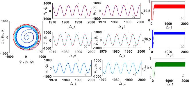
Figure 8. (a) The joint limit-cycle trajectories of the mechanical oscillators. The evolution of the (b) mean values of ${\bar{q}}_{1}(t)$ (red line), ${\bar{q}}_{2}(t)$ (blue dashed line), (c) mean values of ${\bar{p}}_{1}(t)$ (red line), ${\bar{p}}_{2}(t)$ (blue dashed line), (d) quantum synchronization ${S}_{{q}_{12}}(t)$. (e) Mean values of ${\bar{q}}_{1}(t)$ (red line), ${\bar{q}}_{3}(t)$ (cyan dashed line), (f) mean values of ${\bar{p}}_{1}(t)$ (red line), ${\bar{p}}_{3}(t)$ (cyan dashed line), (g) quantum synchronization ${S}_{{q}_{13}}(t)$. (h) Mean values of ${\bar{q}}_{2}(t)$ (blue line), ${\bar{q}}_{3}(t)$ (cyan dashed line), (i) mean values of ${\bar{p}}_{2}(t)$ (blue line), ${\bar{p}}_{3}(t)$ (cyan dashed line), (j) quantum synchronization ${S}_{{q}_{23}}(t)$. Here, we set ηc = 2.5Δ1, Ωc = 3Δ1, E = 100Δ1 and λ = 0.03Δ1. Other parameters are the same as in figure 2. |
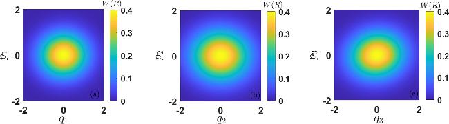
Figure 9. Wigner functions of the three mechanical oscillators. The mean values of the mechanical oscillator's position and momentum are shifted to the origin. The parameter settings are the same as in figure 8. |
3.5. The two types of coupled optomechanical system configurations
As mentioned above, we have identified two configurations among three coupled optomechanical subsystems. One is a linear coupled optomechanical system [see figure 1], and the other is a circular coupled optomechanical system, i.e., the coupling interaction between cavities a1 and a3 is taken into account. Some parameters and energy distributions have different effects in different optomechanical systems. Therefore, we investigate the two coupled optomechanical systems by examining the effects of these parameters and analyzing energy distribution on the quantum synchronization ${S}_{{q}_{13}}$ in different configurations.
As shown in figure 10(a), we investigate the effects of ηc on quantum synchronization ${S}_{{q}_{13}}$ in different optomechanical systems. The green line (yellow line) refers to the quantum synchronization ${S}_{{q}_{13}}$ in the linear (circular) coupled optomechanical system. The effect of modulation amplitude ηc in the circular coupled optomechanical system typically exhibits similar behaviors to that in the linear optomechanical system. As the modulation amplitude ηc varies, the value of quantum synchronization ${S}_{{q}_{13}}$ first increases and reaches a peak when ηc = 2.5Δ1. When ηc crosses this critical value, ${S}_{{q}_{13}}$ decreases as ηc increases. Therefore, as for the two coupled optomechanical systems configurations, we can set ηc = 2.5Δ1 and Ωc = 3Δ1 as the optimal periodic modulation parameters for achieving synchronization. Moreover, it can be shown that ηc has a greater influence on ${S}_{{q}_{13}}$ in a circular coupled system under the specific parameter ranges compared to a linear system.
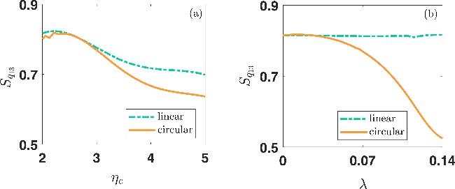
Figure 10. The quantum synchronization of the next-nearest mechanical oscillators ${S}_{{q}_{13}}$ versus (a) the modulation amplitude ηc with Ωc = 3Δ1, λ = 0.03Δ1, (b) the optical coupling strength λ with ηc = 2.5Δ1, Ωc = 3Δ1 in linear (green line) and circular (yellow line) coupled optomechanical systems. Other parameters are the same in figure 2. |
Furthermore, the quantum synchronization ${S}_{{q}_{13}}$ as a function of the cavity coupling strength λ is plotted in figure 10(b). Different from the influence of ηc, the two optomechanical systems exhibit distinct responses to changes in coupling strength λ. In the linear coupled optomechanical system (green line), the coupling interaction has minimal effects on the quantum synchronization ${S}_{{q}_{13}}$ of the next-nearest-neighboring mechanical oscillators. When the coupling strength lies in the large range of 0.01Δ1 to 0.14Δ1, the value of ${S}_{{q}_{13}}$ remains unchanged. In the circular coupled optomechanical system (yellow line), quantum synchronization is sensitive to parameter variations. Quantum synchronization maintains good performance over a small range of coupling strengths (λ < 0.05Δ1). When λ > 0.05Δ1, increasing the coupling strength leads to a continuous decrease in quantum synchronization ${S}_{{q}_{13}}$. Accordingly, we choose λ = 0.03Δ1 as the optimal value for achieving good quantum synchronization in the circular coupled optomechanical system.
In the two optomechanical system configurations, energy distribution and flow mechanisms also exert certain influences on quantum synchronization behaviors. The circular configuration can be modeled as a coupled optomechanical system with periodic boundary conditions, while the linear configuration can be regarded as a coupled optomechanical system with open boundary conditions. The optomechanical system under periodic boundary conditions forms a ring structure. This configuration not only enhances energy flow with reduced boundary losses, but also promotes quantum synchronization through more uniform energy distribution among mechanical oscillators. Moreover, this configuration includes three coupling interaction terms, λ12, λ23 and λ13, which can be regarded as a symmetric coupling configuration. Symmetric coupling will promote the synchronization transmission. When the three coupling coefficients are equal (λ12 = λ23 = λ13), the coupling strength between any two oscillators is identical. This fully symmetric condition makes it easier for all oscillators in the system to achieve global synchronization, wherein all oscillators exhibit identical evolution.
Under open boundary conditions, multiple optical cavities form a linear configuration, where the two end cavities only couple with their adjacent cavity. This configuration may lead to an asymmetric energy distribution. The mechanical oscillators at both ends may be more susceptible to edge effects. Consequently, synchronization is predominantly localized at the two ends, exhibiting better synchronization compared to the middle oscillator. The linear configuration includes two coupling interaction terms, λ12 and λ23, which can be regarded as an asymmetric coupling configuration. Under the influence of asymmetric coupling, the mechanical oscillators at both ends can achieve synchronization transmission by coherent information transfer among the different cavities. If the coupling coefficients are not equal (λ12 ≠ λ23), the mechanical oscillators at both ends will facilitate the anti-synchronization transmission.
3.6. The effects of phonon frequencies and thermal effects on quantum synchronization
Finally, we study the effects of phonon frequency differences and the thermal phonon number on quantum synchronization. In the general synchronization scenario, we find that the phonon frequency of cavities plays a crucial role in assessing synchronization properties. This is due to the fact that a slight frequency variation can induce fluctuations in quantum synchronization. As shown in figure 11(a), quantum synchronization ${S}_{{q}_{13}}$ is numerically evaluated over Δω13/Δ1 ∈ [0.005, 0.0165] under certain modulation ηc = 2.5Δ1, ωc = 3Δ1 and coupling parameters λ1 = λ2 = 0.03Δ1. For a small frequency difference, it is sufficient to achieve synchronization of two mechanical oscillators. An increasing Δω13 leads to degradation of the quantum synchronization ${S}_{{q}_{13}}$. When the frequency difference Δω13 equals 1.65 × 10⁻²Δ1, the synchronization measure ${S}_{{q}_{13}}$ quickly decays to zero, indicating that quantum synchronization behaviors no longer exist. As shown in figure 11(b), when the frequency differences Δω12 and Δω23 are equal to 1.6 × 10⁻²Δ1, the values of quantum synchronization ${S}_{{q}_{12}}$ and ${S}_{{q}_{23}}$ rapidly decrease to zero. Therefore, quantum synchronization occurs when the phonon frequency differences of cavities are smaller than the threshold of 1.6 × 10⁻²Δ1.
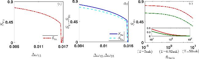


Figure 11. The quantum synchronization as a function of (a) phonon frequency difference Δω13, (b) phonon frequency differences Δω12 and Δω23, (c) mean thermal phonon number ${\bar{n}}_{{\rm{bath}}}$ with ηc = 2.5Δ1, ωc = 3Δ1, λ1 = λ2 = 0.03Δ1 (red line), ηc = 2Δ1, ωc = 2Δ1, λ1 = 0.3Δ1, λ2 = 0.2Δ1 (green line). The temperature values corresponding to a ∼100 MHz oscillator frequency are given. Other parameters are the same in figure 2. |
So far, we set mean thermal phonon number ${\bar{n}}_{{\rm{bath}}}=0$ under a zero-temperature assumption. Next, we will analyze the system's robustness to thermal noise and consider the effects of temperature. As the bath's temperature increases, the mean thermal phonon number will also increase. As shown in figure 11(c), we display the responses of quantum synchronization ${S}_{{q}_{13}}$ as the thermal phonon number ${\bar{n}}_{{\rm{bath}}}$ increases from 10−1 to 101. For a mechanical oscillator with frequency of ∼100 MHz, the corresponding temperature T ranges from approximately 2 mK to 50 mK. It can be seen that the value of the synchronization measure remains stable before ${\bar{n}}_{{\rm{bath}}}\sim 1{0}^{0}$ (corresponding to temperature T = 6.92 mk). Therefore, the relevant experiment may need to be conducted in a low-temperature environment. The inset shows that for a larger ${\bar{n}}_{{\rm{bath}}}$, the synchronization value tends to zero and the synchronization behaviors nearly disappear.
4. The experimental realization of the quantum synchronization in multimode coupled optomechanical systems
The study of quantum synchronization extends beyond theoretical frameworks, and relevant experimental research has also been carried out. These include the synchronization of two different silicon nitride mechanical resonators [111], quantum synchronization in optomechanical arrays [109, 110, 112] and superconducting qubit chain [113]. Recently, long-range synchronization of two optomechanical systems via optical fibers has been experimentally realized and observed [114]. According to the current studies [100, 114], we can provide the parameter settings for the experiment. The frequency of the three mechanical oscillators is ω1/2π ≈ 120.07 MHz, ω2/2π ≈ 120.90 MHz, and ω3/2π ≈ 120.49 MHz. The decay rates of the oscillators and cavities are γ/2π ≈ 110.4 kHz and κ/2π ≈ 3.3 MHz, respectively. The coupling interaction between mechanical oscillators and optical cavities can be realized by colocalized modes. The coupling strength is defined as $g=({\omega }_{{\rm{c}}}/L)\sqrt{\hslash /m{\omega }_{j}}$, where the effective mass of the mechanical mirror is m = 150 ng. In optomechanical systems, g ∼ γ<κ represents a common coupling strength [6, 43]. The coupling interaction between cavities λ ≈ 3 × 10⁻²ωj and the cavity detuning Δj = ωj. The length of the cavity is L = 25 mm, and the finesse is F = 1.4 × 10⁴ [100]. The cavity is driven by a pump laser with an input power of Pin = 280μW. The Q factor of the pump optical mode is Q = 3.56 × 10⁷. We also apply a sinusoidal modulation to the cavity detuning frequency with frequency Ωc ∼ 3ωj and amplitude ηc ∼ 2.5ωj.
According to the current experimental studies, quantum synchronization in arrays of silicon nitride micromechanical oscillators has been experimentally observed [109, 115]. Based on the above studies, mechanical oscillators with slightly different frequencies can be realized by double-disk optomechanical oscillators, which are composed of two independent silicon nitride circular edges [116, 117]. The driving laser can be achieved by placing a tapered optical fiber in the optical cavity of an optomechanical array [109]. When a continuous-wave laser drives optical cavities, the continuously and stably output laser ensures the self-sustained oscillation, and provides the essential optomechanical coupling required for synchronization. When the driving frequency of the laser exceeds the oscillation threshold, the silicon nitride edges exhibit coherent oscillations and synchronization. The coupling interaction between optical cavities can be achieved via optical supermodes, and the mechanical oscillators are coupled through the evanescent field [109]. In addition, coupling between adjacent optical cavities can be achieved via optical fibers. The coupling interaction between next nearest neighbor optical cavities, has also been taken into account in some studies [118, 119]. The long-range coupling interaction may have challenges in practice. According to some current studies [118], when the optomechanical system forms a cyclic structure, long-range coupling interactions can be changed into coupling between two adjacent cavities. Some studies also suggest that long-range coupling can be achieved through optical fiber loop [120].
5. Conclusion
In summary, we study quantum synchronization and synchronization transmission in a coupled multimode optomechanical system. Through the joint limit-cycle trajectories and Wigner function of three mechanical oscillators, we can visualize tripartite synchronization in a multimode optomechanical system. Moreover, quantum synchronization and quantum anti-synchronization between two mechanical oscillators can also be achieved simultaneously by manipulating the driving laser. Therefore, driving laser is a prerequisite for achieving quantum synchronization. Accordingly, we can utilize lasers to manipulate synchronization transmission between mechanical oscillators, and we anticipate that this method can also be generalized to optomechanical chains. We also present the parameter ranges for achieving good quantum synchronization in the three-coupled optomechanical system. According to different configurations, we extend this model to a circular coupled optomechanical system. In this configuration, any two mechanical oscillators can achieve quantum complete synchronization. In addition, the effects of parameters and energy distribution in the two types of coupled multimode optomechanical systems are analyzed. We also investigate the effects of phonon frequency and thermal phonon numbers on quantum synchronization. Finally, we discuss the experimental parameters and implementation of quantum synchronization in the multimode coupled optomechanical system.
We believe that our findings are also applicable to other coupled optomechanical systems, such as a system with four cavities and four oscillators, where two pairs of cavities are connected in a ring in alternating order. This extension is feasible as the number of coupled optomechanical subsystems continues to increase. For a one-dimensional optomechanical lattice consisting of N optical cavities and N mechanical oscillators, synchronization transmission can also be achieved. Moreover, quantum synchronization transmission has potential applications in quantum information processing and quantum control.