

1. Introduction
2. Evaporation of primordial black holes
3. Cosmic ray propagation
3.1. Cosmic ray propagation in the galaxy
3.2. Cosmic ray propagation in the heliosphere
3.3. Benchmark propagation models
DRz4-10 models. Four diffusive re-acceleration models with different zh (fixed to 4, 6, 8, 10 kpc, respectively). As discussed above, the values of zh are selected to illustrate the affect of zh on the obtained constraints on fPBH. We have four free parameters for CR propagation, which are D0 (normalized at 4 GV), η, δ, and Va.
DBz4 model. A diffusion break model with zh fixed to 4 kpc. We have four free parameters for CR propagation, which are D0 (normalized at 4 GV), ρl, δl and δ. In this model, Va is fixed to zero.
GH model. The model was built with analysis framework of
Table 1. Model parameters, and their prior ranges, posterior means and standard deviations (show in brackets) of the benchmark models. |
| Parameter | Prior range | DBz4 | DRz4 | DRz6 | DRz8 | DRz10 |
|---|---|---|---|---|---|---|
| D0 (1028 cm2 s−1) | [1, 10] | 4.23 (0.18) | 4.20 (0.17) | 5.86 (0.23) | 7.04 (0.28) | 7.84 (0.31) |
| ρl (GV) | [0.5, 10] | 5.12 (0.36) | — | — | — | — |
| δl | [−1, 0] | −0.374 (0.090) | — | — | — | — |
| δ | [0.2, 0.6] | 0.490 (0.008) | 0.440 (0.011) | 0.437 (0.011) | 0.436 (0.011) | 0.435 (0.011) |
| η | [−2, 2] | — | −0.628 (0.137) | −0.607 (0.135) | −0.595 (0.134) | −0.583 (0.138) |
| Va (km s−1) | [0, 60] | — | 21.1 (1.7) | 20.7 (1.7) | 20.1 (1.7) | 19.5 (1.6) |
| γ0 | [0.2, 3.2] | 0.885 (0.122) | 0.848 (0.116) | 0.869 (0.111) | 0.879 (0.113) | 0.885 (0.111) |
| γ1 | [1.8, 3.2] | 2.346 (0.008) | 2.369 (0.008) | 2.372 (0.008) | 2.373 (0.008) | 2.374 (0.008) |
| ρ0 (GV) | [0.1, 20] | 1.52 (0.11) | 1.54 (0.10) | 1.54 (0.10) | 1.54 (0.10) | 1.54 (0.09) |
| AC12 | [1000, 6000] | 3487 (28) | 3421 (28) | 3410 (28) | 3407 (28) | 3404 (28) |
| φ (MV) | [0, 1500] | 470 (27) | 606 (27) | 606 (26) | 605 (26) | 605 (26) |
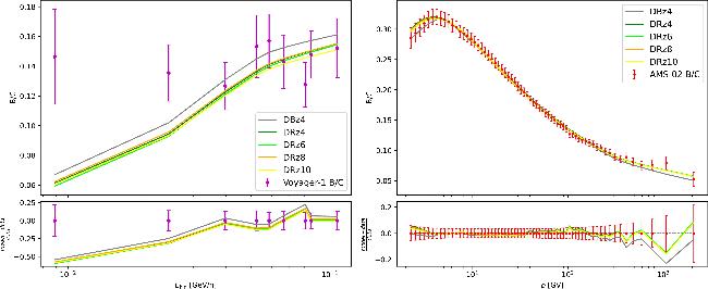
Figure 1. Model predictions and residuals of B/C flux ratio for the benchmark models. Left: for Voyager-1. Right: for AMS-02. |
Table 2. Model parameters relevant to the calculation of synchrotron signals of PBHs for CR propagation models adopted in this work. |
| Parameter | DBz4 | GH [79] | DRz4 | DRz6 | DRz8 | DRz10 |
|---|---|---|---|---|---|---|
| zh (kpc) | 4 | 4 | 4 | 6 | 8 | 10 |
| D0 (1028 cm2 s−1) | 4.23 | 4.3 | 4.20 | 5.86 | 7.04 | 7.84 |
| ρl (GV) | 5.12 | — | — | — | — | — |
| δl | −0.374 | — | — | — | — | — |
| δ | 0.490 | 0.415 | 0.440 | 0.437 | 0.436 | 0.435 |
| η | — | 0.7 | −0.628 | −0.607 | −0.595 | −0.583 |
| Va (km s−1) | — | 30 | 21.1 | 20.7 | 20.1 | 19.5 |
| dV/dz (km s−1 kpc−1) | — | 9.8 | — | — | — | — |
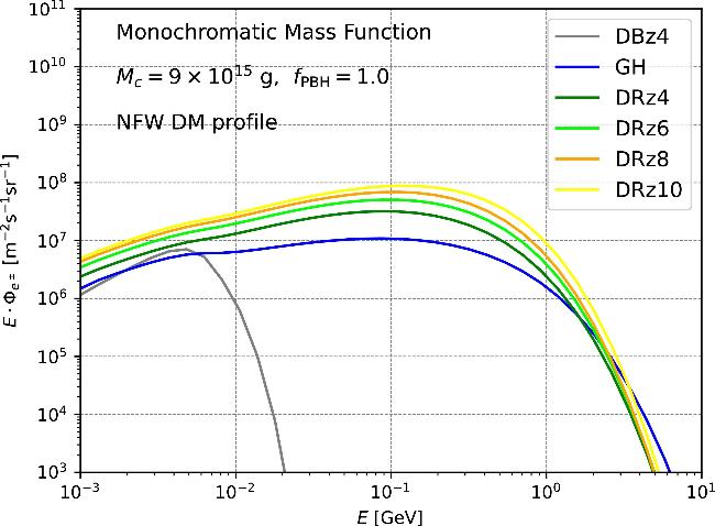
Figure 2. The LIS energy spectra of evaporated all-electrons at the Solar position for CR propagation models adopted in this work, assuming a monochromatic mass function with Mc = 9 × 10¹⁵ g, fPBH = 1.0, and NFW DM profile. |
4. Synchrotron emission and GMF models
4.1. Basic physical processes
4.2. GMF models
SUNE model. The model of the same name constructed in [154]. It utilizes the best-fit regular field from [170, 171], including the ASS + RING disc field and an updated toroidal halo field from [171]. Its striated random field aligns with the regular field and maintains a constant strength ratio relative to the strength of regular field through out the Galaxy. The isotropic random field decreases exponentially in both radial and vertical directions. The random field parameters are fitted using the radio continuum surveys from 22 MHz to 2.3 GHz, and the total and polarized intensity data from 7 year Wilkinson Microwave Anisotropy Probe (WMAP) at frequencies between 23 GHz and 94 GHz. The WMAP MCMC templates are adopted to account for dust and spinning-dust emissions. Free–free absorption and emission are computed with specific interstellar ionized gas model, and the CR electron density follows the z04LMPDS model in [172].
JF12 model. A more complex model constructed in [162, 163]. Its regular field includes: 1. a disc field with eight spiral arms, 2. a toroidal halo field, 3. an X-shaped halo field extending perpendicular to the Galactic plane. The striated random field is parameterized by a parameter β in the whole galaxy, defined as the striated-to-regular emission ratio. We use the updated value of β in [163]. The isotropic random field includes: 1. a disc field mirroring the structure of the regular disc field, 2. a halo field combining radial exponential and vertical Gaussian profiles. The random field parameters are fitted using the total and polarized intensity data from the 7 year WMAP at 23 GHz, and with the assumption of a constant spectral index α = 3 for CR electron density.
5. Constraints on the PBH abundance
5.1. Observational data and error estimation
22 MHz. Dominion Radio Astrophysical Observatory Northern Hemisphere survey [173].
45 MHz. Northern sky: Japanese Middle and Upper Atmosphere radar array [174], Southern sky: Maipú Radio Astronomy Observatory 45 MHz array [175], and the combined all-sky map from [176].
85 MHz. Parkes radio telescope [177].
150 MHz. Parkes–Jodrell Bank all-sky survey [177].
408 MHz. Bonn–Jodrell Bank–Parkes all-sky survey [178], and reprocessed by [179].
850 MHz. Dwingeloo telescope [180].
1420 MHz. Northern sky: 25 m Stockert telescope [181, 182], Southern sky: 30 m Villa-Elisa telescope [183, 184].
All datasets are publicly accessible on the LAMBDA website.7 The observed intensity is recorded in the sky map of brightness temperature T(ν), which is converted from the intensity I(ν) as5.2. Synchrotron signals of PBHs
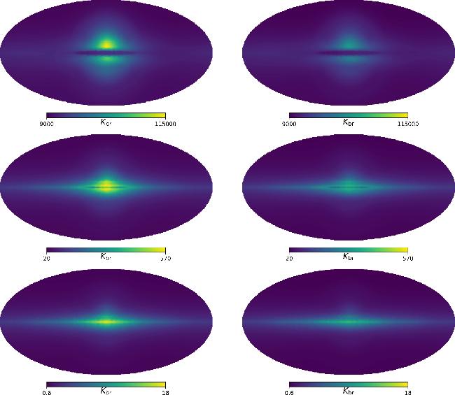
Figure 3. Sky maps of synchrotron signals of PBHs with NFW and Burkert DM profiles (left and right) at 22 MHz, 150 MHz, and 408 MHz (top to bottom), assuming a monochromatic mass function with Mc = 5 × 10¹⁴ g, GH CR propagation model, and SUNE GMF model. All maps are computed with fPBH = 10−8, and are plotted with Nside = 64 and linear color mapping. |
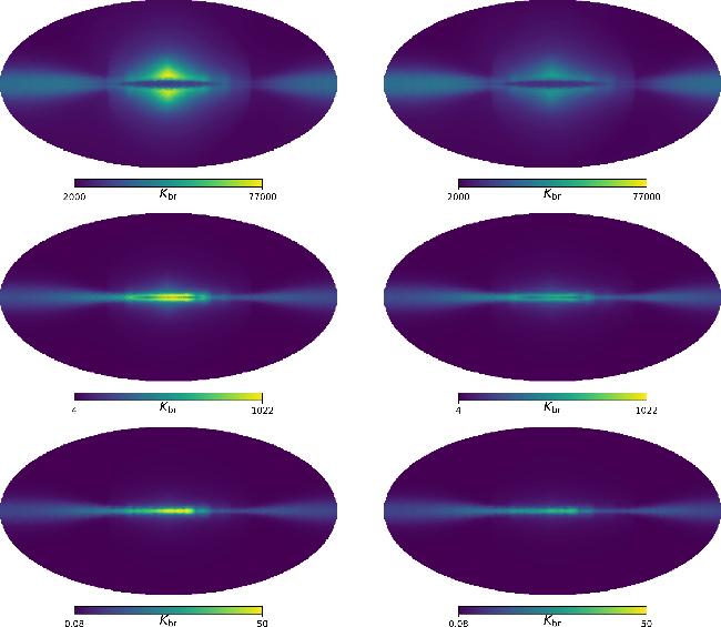
Figure 4. Same as figure 3 but for JF12 GMF model. |
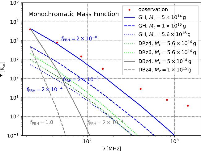
Figure 5. Spectra of synchrotron signals of PBHs for GH, DRz4, DRz6 and DBz4 CR propagation models, assuming SUNE GMF model, NFW DM profile, and monochromatic mass functions of selected Mc = 5 × 10¹⁴ g, 1 × 10¹⁵ g, and 5.6 × 10¹⁶ g. The spectra are averaged within the intermediate latitudes 10∘ < ∣b∣ < 40∘. Observed intensities averaged within the same region are also shown. For a tight plot, the spectra of GH model are scaled by fPBH = 2 × 10⁻⁸, 2 × 10⁻⁸ and 2 × 10⁻⁴ for each Mc, and the spectra of DBz4 model are scaled by fPBH = 2 × 10⁻⁴ and 1.0 for the smaller two Mc (as labeled). Only the spectra with Mc = 5.6 × 10¹⁶ g for DRz4 and DRz6 models are shown, which are also scaled by fPBH = 2 × 10⁻⁴ as the spectrum of GH model with the same Mc (the fPBH is not labeled). |
5.3. Results
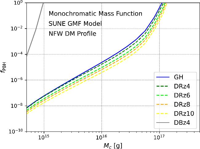
Figure 6. Constraints on fPBH for different CR propagation models, assuming monochromatic mass functions, SUNE GMF model, and NFW DM profile. |
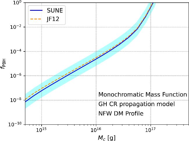
Figure 7. Constraints on fPBH for SUNE and JF12 GMF models, assuming monochromatic mass functions, GH CR propagation model, and NFW DM profile. The shaded region illustrates the impact of varying the overall normalization of the SUNE magnetic field by a factor of two on the resulting constraints. |
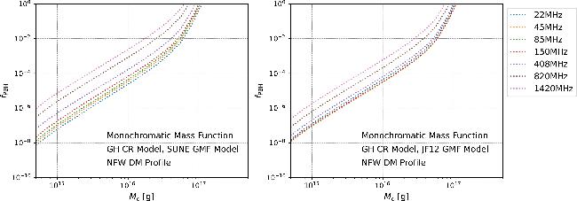
Figure 8. Constraints on fPBH derived from individual observational sky maps, assuming monochromatic mass functions, GH CR propagation model, and NFW DM profile. Left: for SUNE GMF model. Right: for JF12 GMF model. |
For the SUNE model. In the 22 MHz ratio map, the region ∼30∘ above the Galactic center within ∼10∘ radius, corresponding to the dark area enclosed by the North Polar Spur in the observational sky map.
For the JF12 model. In the 150 MHz ratio map, the region ∼15∘ below and above the Galactic disc at longitudes 240∘ < l < 300∘, corresponding to the dark area on the Galactic disc at the same longitudes in the observational sky map.
Note that in the right panel of figure 8, the constraints derived from the 22 MHz observational sky map for the JF12 model are slightly weaker than the strongest constraints, because the outer-disc region (at longitudes 240∘ < l < 300∘) absents in the 22 MHz observational sky map. The difference between the most constraining sky regions for these two GMF models likely origins from JF12's prominent disc random field (especially in 6th and 7th spiral arms), which yields larger synchrotron signals on the Galactic disc.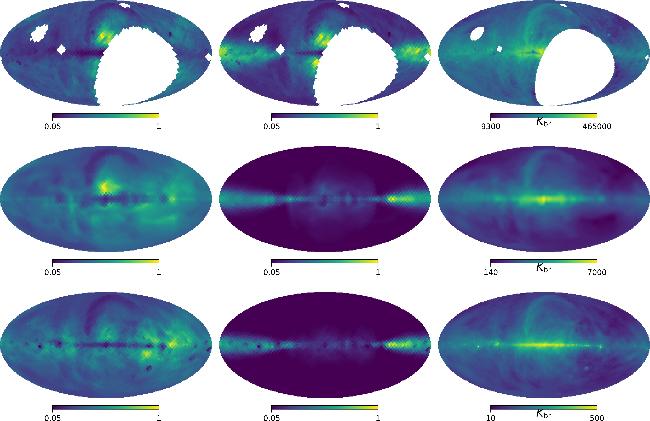
Figure 9. The first two columns: ratio of synchrotron signals to observational limits (intensity + 2 × error) at 22, 150 and 408 MHz (top to bottom) for SUNE and JF12 GMF models, respectively, assuming a monochromatic mass function with Mc = 5 × 10¹⁴ g, GH CR propagation model, and NFW DM profile. Synchrotron signals are scaled by specific values of the constraints on fPBH derived from individual observational sky maps such that ratio = 1 corresponds to the pixel where the constraint is obtained. All maps are plotted with Nside = 16 and linear color mapping. The last column: the 22, 150 and 408 MHz (top to bottom) observational sky maps for comparison, plotted with original resolution and logarithmic color mapping. |
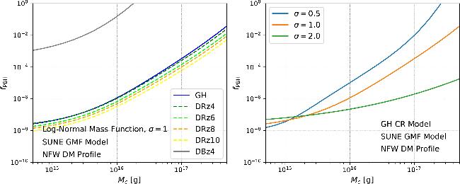
Figure 10. Constraints on fPBH with log-normal mass functions. Left: for different CR propagation models, assuming the distribution width σ = 1, SUNE GMF model, and NFW DM profile. Right: for different distribution widths σ = 0.5, 1.0, and 2.0, assuming GH CR propagation model, SUNE GMF model, and NFW DM profile. |
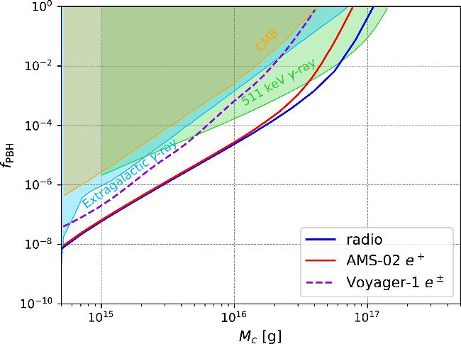
Figure 11. Several constraints on fPBH with monochromatic mass functions. Shadow regions show constraints derived from different observables, including extragalactic γ-rays [52], CMB [26], and 511 keV γ-rays [59]. Lines show constraints derived from Voyager-1 all-electrons data [70], AMS-02 positron data [71], and radio continuum surveys (assuming GH CR propagation model, SUNE GMF model, and NFW DM profile). |
6. Conclusion
Appendix A Fit results for benchmark models
A.1. Numerical details
A.2. Extended results
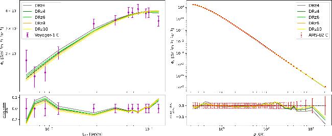
Figure 12. Model predictions and residuals of C flux for the benchmark models. Left: for Voyager-1. Right: for AMS-02. |
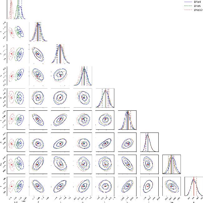
Figure 13. Corner plots of posterior PDFs for DRz4, DRz6, and DRz10 models. The result of DRz8 model is excluded for clarity. Contours show 1 and 2-σ credible regions of 2D distributions, containing 39.3% and 86.4% of the posterior probability mass, respectively. Points mark the posterior means, and crosses mark the maximum posterior values. In 1D marginalized posterior plots, solid vertical lines show the posterior means, and dotted vertical lines show positions of the posterior mean ± standard deviation. For a tight plot, D0 is replaced with D0/zh (with unit: 1028 cm2 s−1 kpc−1). |
Appendix B Extended results for constraints on the PBH abundance
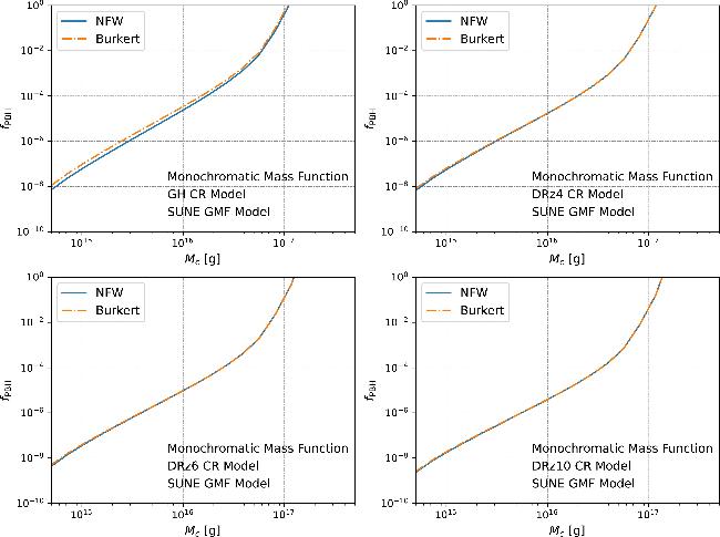
Figure 14. Constraints on fPBH for different DM profiles and for different CR propagation models (as labeled), assuming monochromatic mass functions and SUNE GMF model. The plot for DRz8 model is omitted. |
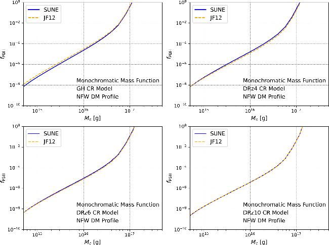
Figure 15. Constraints on fPBH for different GMF models and for different CR propagation models (as labeled), assuming monochromatic mass functions and NFW DM profile. The plot for DRz8 model is omitted. |
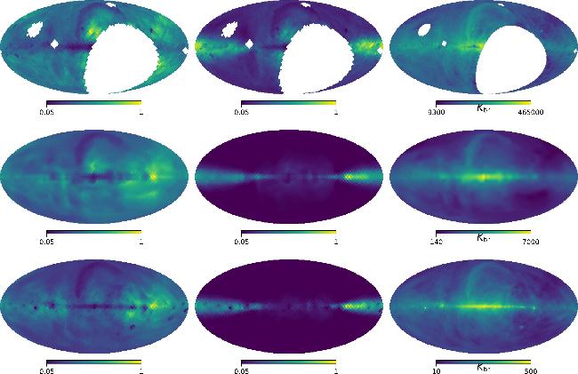


Figure 16. Same as figure 9 but for Burkert DM profile. |