

1. Introduction
Dark matter (DM) constitutes approximately 85% of the total matter in the Universe, and its existence is firmly established through gravitational effects such as galactic rotation curves, gravitational lensing, and cosmic microwave background anisotropies [1–5]. However, the fundamental nature of DM—whether it is composed of weakly interacting massive particles (WIMPs) [6], axions [7–9], ultra-heavy particles, or other exotic entities—remains one of the most pressing unsolved problems in modern physics. To unravel this mystery, a diverse array of experimental strategies has been developed, including direct detection (e.g. LZ, XNON, PANDAX) [10–13], indirect detection (e.g. LHAASO) [14], and collider searches (e.g. LHC) [15, 16]. Despite decades of efforts, no conclusive signal of DM has been detected, highlighting the need for complementary detection approaches that can probe uncharted regions of DM parameter space. Terrestrial detectors, while powerful, face inherent limitations in exploring certain DM regimes. Direct detection experiments (CDEX, PANDAX) operating underground are highly sensitive to low-to-intermediate mass DM (GeV–TeV scale) but struggle with ultra-heavy DM (UHDM, m ≳ 103 GeV) due to the extremely low collision rate and limited detector mass. Indirect detection experiments (LHAASO) search for secondary particles from DM annihilation/decay but are plagued by astrophysical backgrounds that complicate signal interpretation [17]. Collider experiments, on the other hand, are restricted by their center-of-mass energy, making them unable to produce UHDM particles directly.
Space-based gravitational wave (GW) detectors, such as China's Taiji mission [18] (in a heliocentric orbit) and TianQin mission [19] (which operates in a geocentric orbit), and the European LISA mission [20] (in a heliocentric orbit), offer a unique opportunity to bridge this gap. The distinct orbital configurations will lead to different annual modulations of the DM signal, as discussed in section 2.2.4 , providing an additional handle for signal identification. These detectors are designed to measure GWs from compact binary coalescences and other cosmic sources with ultra-high precision, relying on the stable motion of test masses (TMs) in ultra-high vacuum and microgravity environments . Unlike terrestrial detectors, the TMs in space-based interferometers are minimally disturbed by environmental noise, rendering them sensitive to subtle displacements induced by DM collisions—an effect that is negligible or masked in ground-based facilities. Early theoretical studies have suggested that space-based GW detectors could be repurposed as ultralight DM probes [21–23], but a comprehensive theoretical framework describing TM motion induced by DM collisions across diverse scenarios (e.g. stochastic collisions, Brownian motion) has been lacking.
In this work, we address these gaps by establishing a rigorous and unified theoretical framework to characterize TM motion driven by DM collisions in space-based GW detectors. Our key contributions are as follows: (1) We analyze three representative collision scenarios (synchronous coherent collisions, stochastic unidirectional flux, and stochastic isotropic flux) to cover the full range of DM interaction regimes. (2) We identify a universal 1/f4 power spectral density (PSD) of TM displacement as a signature of DM-induced motion, which is distinct from GW signals and instrumental noise. (3) For the physically relevant isotropic flux scenario, we derive a key scaling relation mσ = constant at the signal-to-noise ratio (SNR) threshold, providing a robust constraint on DM properties. (4) We unify time-domain (stochastic differential equations) and frequency-domain (PSD) descriptions using the Wiener–Khinchin theorem, verifying their mathematical consistency. (5) We extend the framework to Brownian motion formalism, incorporating the Standard Halo Model (SHM) velocity distribution and the observer's velocity boost.
This paper is structured as follows: section 2 derives the equation of motion for the TM and its frequency-domain displacement under a single DM collision and three collision scenarios, focusing on the PSD and SNR constraints. Section 3 extends the framework to light DM-induced Brownian motion with a rigorous mathematical derivation. In section 4 we relate the single TM motion to the actual interferometric observable—the differential displacement—and demonstrate that the key spectral features remain unchanged. Section 5 discusses experimental realities such as damping and feedback control. Section 6 proposes a scalable experimental framework for massive DM detection. Section 7 presents the conclusions. Appendix A verifies the equivalence between time-domain and frequency-domain descriptions.
It is instructive to compare our work with the influential study by Cheng, Primulando, and Spinrath (CPS) [24], which introduced the concept of DM-induced Brownian motion. While both works share this conceptual inspiration, they differ fundamentally in scope, methodology, and target parameter space. First, CPS focuses on light DM (${ \mathcal O }(10)$ MeV) using hypothetical ground-based experiments with ultra-light targets (10−3 g), explicitly ruling out existing detectors like LIGO. Our work, conversely, targets ultra-heavy DM (≳103 GeV) by repurposing existing space-based GW detectors (Taiji, LISA)—a mass regime completely inaccessible to their approach. Second, the observable and framework are distinct. CPS proposes resolving individual recoil events in the time domain to extract a directional asymmetry A. Our work treats collisions as a stochastic process in the frequency domain, deriving a universal 1/f4 PSD and the scaling relation mσ = constant—results that are mathematically inaccessible in their framework. Thus, rather than overlapping, our works are highly complementary: CPS explores a novel technique for light DM, while ours establishes a comprehensive framework for probing the UHDM frontier using next-generation space interferometers.
2. Test mass motion induced by dark matter collisions
We begin by analyzing the motion of a single TM driven by DM collisions. This serves as the fundamental building block for the interferometric observable. In practice, space-based detectors measure the differential displacement Δx = x2 − x1 between two free-falling TMs at the ends of each arm. For ultra-heavy DM, the two TMs experience statistically independent stochastic forces (see section 4 ). for rigorous proof), yielding SΔx(f) = 2Sx(f). Thus, the single-TM analysis directly translates to the differential signal with a factor-of-2 enhancement in the PSD.
In contrast to terrestrial GW detectors, such as the Advanced Laser Interferometer Gravitational-Wave Observatory (aLIGO) [25], the Kamioka Gravitational Wave Detector [26], and the proposed Einstein Telescope (ET) [27, 28], space-based GW detectors [18, 29] exhibit distinct response characteristics to DM interactions. This distinction arises primarily from their unique operational environment characterized by ultra-high vacuum, microgravity, and large-scale orbital configurations—which renders space-based detectors sensitive to DM-induced signals that may be negligible or undetectable in terrestrial facilities.
A crucial aspect of signal formation must be addressed: interferometers measure the differential displacement between widely separated TMs. If DM imparted identical motion to all components, it would constitute a common-mode signal and cancel out. Detectability relies on differential coupling—e.g. different material compositions of TMs and spacecraft—which ensures a net relative displacement. This differential nature, combined with fundamental operational differences, explains why ground-based detectors are intrinsically unsuited for the signal considered here. First, their sensitive frequency band lies above ∼10 Hz, where seismic and suspension noise dominate, whereas the predicted 1/f4 signal peaks in the millihertz range accessible only in space. Second, ground-based TMs are pendulously suspended, introducing resonances and damping that suppress low-frequency responses, unlike freely falling space TMs with a clean 1/f2 transfer function. Third, their kilometer-scale arms imply that a single DM particle could correlate the motion of both TMs for weak interactions, causing correlated motion that is partially suppressed in the differential measurement—a problem largely avoided by the 3 × 10⁹ m arms of Taiji/LISA, which ensure interactions at the two TMs are effectively independent. These physical constraints render terrestrial interferometers insensitive to the DM signal considered here, while space missions offer a unique window for such searches.
However, a detectable differential signal arises from the fact that the TMs and the spacecraft are macroscopic bodies with different compositions, geometries, and shielding environments. The coupling to DM, characterized by the scattering cross-section σ, is material-dependent. Consequently, the impulsive force exerted by a DM particle on a gold-platinum TM (FTM depends on σTM/MTM) will differ from that on a spacecraft made primarily of titanium or carbon-fiber reinforced plastic (FSC depends on σSC/MSC). This differential coupling ensures that DM collisions produce a net relative displacement Δx = xTM − xSC that can be registered by the laser interferometer just like in [30] which may cause new detectable signal. Our theoretical framework, which focuses on the motion of a single TM, should be interpreted as the first step in modeling this differential signal. A complete analysis would require convolving the single-TM response with the detector's transfer function for differential modes, while incorporating the distinct coupling strengths of the TM and SC materials. For simplicity and to establish an upper limit on sensitivity, this work proceeds with the single-TM analysis, noting that the derived 1/f4 spectral shape is expected to persist in the differential signal, albeit with a modified amplitude that depends on the material-specific coupling contrast. A detailed treatment of this differential effect is planned for future work.
2.1. Equation of motion for the test mass
To quantitatively characterize the effect of DM collisions on a TM in space, we adopt an impulsive force model to describe the interaction between DM particles and the TM. For a single DM particle with mass m colliding with the TM at a relative velocity v, the impulsive force exerted on the TM can be rigorously described by the Dirac delta function, i.e. F(t) = mvδ(t) [31, 32], where δ(t) denotes the Dirac delta function that encapsulates the instantaneous nature of the collision [33]. For a TM with mass M, the equation of motion governed by Newton's second law is thus expressed as:
$\begin{eqnarray}M\ddot{x}=F=mv\delta (t).\end{eqnarray}$
To facilitate the analysis of the TM's displacement in the frequency domain—where the sensitivity of space-based interferometers is typically evaluated—we apply the Fourier transform to both sides of the above equation. Utilizing the Fourier transform property ${ \mathcal F }\{\ddot{x}(t)\}=-{(2\pi f)}^{2}x(f)$ [34] (where f denotes the frequency and x(f) is the Fourier transform of the time-domain displacement x(t)) and ${ \mathcal F }\{\delta (t)\}=1$, we obtain: $\begin{eqnarray}M{(2\pi f)}^{2}x(f)=mv.\end{eqnarray}$
Rearranging this expression to solve for the frequency-domain displacement x(f), we derive the core relation describing the TM's response to a single DM collision: $\begin{eqnarray}x(f)=\frac{mv}{M{(2\pi f)}^{2}}.\end{eqnarray}$
Notably, this signal profile exhibits a 1/f2 dependence on frequency, which is distinctly different from the typical GW signals targeted by space-based interferometers (e.g. Taiji), whose frequency-domain profiles are governed by the orbital dynamics of compact binary systems and do not follow this inverse-square frequency scaling. We note that the minus sign in x(f) does not affect the PSD, which depends on ∣x(f)∣2.A more complete equation of motion that includes weak restoring and dissipative forces is [35]
$\begin{eqnarray}M\ddot{x}+\gamma \dot{x}+kx={F}_{{\rm{DM}}}(t),\end{eqnarray}$
where γ is the damping coefficient and $k=M{\omega }_{0}^{2}$ is the effective spring constant corresponding to a characteristic resonant frequency ω0. For Taiji, the TMs are designed to be free-falling above f ≳ 10−4 Hz, implying ω0/(2π) ≲ 10−4 Hzw hich corresponds to the lower bound of Taiji's sensitive frequency band [18] and γ/(2πM) ≪ 10−4 Hz. The transfer function in the frequency domain becomes $\begin{eqnarray}\begin{array}{rcl}H(f) & = & \frac{1}{M{(2\pi f)}^{2}-k-{\rm{i}}(2\pi f)\gamma }\\ & = & \frac{1}{M\left[{(2\pi f)}^{2}-{\omega }_{0}^{2}-{\rm{i}}(2\pi f)\gamma /M\right]}.\end{array}\end{eqnarray}$
2.2. Collision scenarios in a one-dimensional model
To comprehensively assess the TM motion induced by DM collisions, we construct a one-dimensional model and analyze three representative collision scenarios: fully synchronous coherent collisions (an extreme upper-limit case), stochastic collisions with unidirectional DM flux (a simplified realistic case), and stochastic collisions with isotropic DM flux (the most physically relevant case). This hierarchical analysis allows us to quantify the range of possible TM responses and derive robust constraints on DM properties.
2.2.1. Synchronous coherent collisions
We first consider the hypothetical scenario of fully synchronous and coherent DM collisions, which serves as the upper bound for the TM displacement induced by a given number of DM particles. Let R denote the collision rate (i.e. the number of collisions per unit time per unit mass of the TM). Over an observation time T, the total number of DM particles colliding with the TM is N = RMT [31, 36], where MT accounts for the product of the TM mass and observation duration. We first assume the DM flux is isotropic, leading to random directionality of individual collision impulses; as a result, the mean displacement of the TM over many collisions is zero due to mutual cancellation of impulses in opposite directions. However, to establish the maximum possible TM displacement (a critical benchmark for detector sensitivity), we impose the hypothetical condition that all N DM particles collide with the TM simultaneously and coherently, such that their impulses add constructively along the measurement axis. Under this condition, the total momentum transferred to the TM is P = Nmv. Substituting this total momentum into the frequency-domain displacement formula derived in the previous section, the TM displacement becomes:
$\begin{eqnarray}x(f)=\frac{Nmv}{M{(2\pi f)}^{2}}.\end{eqnarray}$
While this fully coherent scenario is highly improbable in nature—requiring fine-tuning of DM particle arrival times and directions—it provides a rigorous limit on the TM displacement for a given collision rate R and observation time T, which is valuable for assessing the best-case signal contamination in space-based GW detectors.2.2.2. Stochastic collisions: unidirectional flux case
A more physically realistic scenario involves stochastic DM collisions, where N collisions occur at distinct, random times tj (j = 1, 2, …, N) over the observation time T. In this case, the total impulsive force exerted on the TM is the superposition of individual collision forces, leading to the following equation of motion: 7 ) and utilizing the time-shifting property of the Fourier transform ${ \mathcal F }\{\delta (t-{t}_{j})\}={{\rm{e}}}^{-{\rm{i}}2\pi f{t}_{j}}$, we obtain the frequency-domain relation: 8 ) as a two-dimensional random walk process the sum of complex exponential in equation (8 ) as a two-dimensional random walk process, where each term ${{\rm{e}}}^{-{\rm{i}}{\phi }_{j}}$ corresponds to a step of unit length in the complex plane with random direction.
$\begin{eqnarray}M\ddot{x}=\displaystyle \sum _{j=1}^{N}mv\delta (t-{t}_{j}).\end{eqnarray}$
Applying the Fourier transform to both sides of equation ( $\begin{eqnarray}M{(2\pi f)}^{2}x(f)=mv\displaystyle \sum _{j=1}^{N}{{\rm{e}}}^{-{\rm{i}}2\pi f{t}_{j}}.\end{eqnarray}$
For large N ≫ 1 (a valid approximation for typical DM flux densities and observation times in space-based detectors), we model the collision times tj as independent and identically distributed random variables, following a uniform distribution over the interval [0, T]. This corresponds to a Poisson process for the collisions, which is the standard assumption for a homogeneous DM halo. Consequently, the phases φj = 2πftj are also independent and uniformly distributed over [0, 2πfT]. For frequencies of interest, f ≫ 1/T, the phases effectively cover the full [0, 2π] range uniformly. This allows us to model the sum of complex exponential in equation (Based on the central limit theorem for random walks, the sum of N such independent random terms can be approximated as [37]: 9 ) into equation (8 ) and rearranging to solve for x(f), we obtain the frequency-domain displacement for stochastic unidirectional collisions: 10 ) into the PSD definition and utilizing the property ⟨α2⟩ = 2 for a standard Rayleigh distribution, we derive:
$\begin{eqnarray}\displaystyle \sum _{j=1}^{N}{{\rm{e}}}^{-{\rm{i}}2\pi f{t}_{j}}=\sqrt{\frac{N}{2}}\,\alpha \,{{\rm{e}}}^{-{\rm{i}}\varphi },\end{eqnarray}$
where α follows a standard Rayleigh distribution (with probability density function ${p}(\alpha )=\alpha {{\rm{e}}}^{-{\alpha }^{2}/2}$ for α ≥ 0) and φ is uniformly distributed over [0, 2π]. Substituting equation ( $\begin{eqnarray}x(f)=\frac{mv}{M{(2\pi f)}^{2}}\sqrt{\frac{N}{2}}\,\alpha \,{{\rm{e}}}^{-{\rm{i}}\varphi }.\end{eqnarray}$
It is important to note that while the ensemble average of the frequency-domain displacement ⟨x(f)⟩ is zero (due to the randomness of φ), the time-domain motion ⟨x(t)⟩ is non-zero. This is because the TM acquires a constant velocity between consecutive collisions, and the cumulative effect of these velocity increments (even with random signs) leads to a non-vanishing mean displacement over time. To quantify the statistical properties of the TM displacement, we compute its PSD, defined as the limit of the ensemble average of the squared magnitude of x(f) divided by the observation time T as T → ∞. Substituting equation ( $\begin{eqnarray}{S}_{x}(f)=\mathop{\mathrm{lim}}\limits_{T\to \infty }\frac{\left\langle | x(f){| }^{2}\right\rangle }{T}=\frac{{m}^{2}\langle {v}^{2}\rangle N}{T{M}^{2}{(2\pi f)}^{4}}=\frac{{m}^{2}\bar{{v}^{2}}N}{T{M}^{2}{(2\pi f)}^{4}},\end{eqnarray}$
where $\bar{{v}^{2}}$ is the assemble average of v2.The 1/f4 dependence in equation (11 ) is a hallmark of this scenario, corresponding to a Brownian motion in the TM's velocity (which exhibits a 1/f2 PSD) integrated twice to obtain displacement consistent with the stochastic nature of impulse-driven motion in section 3 . Including weak damping and restoring forces, the PSD of the TM displacement becomes
$\begin{eqnarray}\begin{array}{rcl}{S}_{x}(f) & = & | H(f){| }^{2}{S}_{F}(f)\\ & = & \frac{{m}^{2}\bar{{v}^{2}}R}{{M}^{2}}\cdot \frac{1}{{\left[{(2\pi f)}^{2}-{\omega }_{0}^{2}\right]}^{2}+{(2\pi f\gamma /M)}^{2}}.\end{array}\end{eqnarray}$
In the frequency regime most relevant for Taiji's DM search, f ≫ f0 ≡ ω0/(2π) and f ≫ fdamp ≡ γ/(4πM), the transfer function simplifies to $| H(f){| }^{2}\approx {[M{(2\pi f)}^{2}]}^{-2}$, recovering our original 1/f4 scaling. For Taiji, with f0 ∼ 10−4 Hz and fdamp even smaller, the signal-rich band from 10−4 to 10−1 Hz safely satisfies this condition. Therefore, the 1/f4 signature remains a robust prediction for the observable frequency range.
To derive constraints on DM properties from the TM's motion, we utilize the SNR formalism commonly employed in GW detector analysis. The SNR is defined as [38]: 25 ). This spectral similarity presents a challenge for signal extraction, as a simple spectral shape analysis may not suffice to distinguish DM from instrumental artifacts. It will be discussed in 2.2.4 . The power PSD of the TM displacement induced by DM collisions, compared with the Taiji and LISA noise is shown in figure 1.
$\begin{eqnarray}{\,\rm{SNR}\,}^{2}=4{\int }_{0}^{\infty }\frac{{S}_{{\rm{\Delta }}x}(f)}{{L}^{2}{S}_{n}(f)}{\rm{d}}f=8{\int }_{0}^{\infty }\frac{{S}_{x}(f)}{{L}^{2}{S}_{n}(f)}{\rm{d}}f,\end{eqnarray}$
where L = 3 × 10⁹ m is the arm length of the Taiji space-based GW detector, and Sn(f) is the total noise PSD of the detector. This noise PSD is dominated by two components: The first one is related to optical metrology system (oms)noise Soms, which dominates at high frequency. These condone is the TM acceleration noise (acc) Sacc that dominates at low frequency. The magnitudes of oms and acc noises are given by [38]: $\begin{eqnarray}{S}_{\,\rm{oms}\,}={\left({s}_{\,\rm{oms}\,}\frac{2\pi f}{c}\right)}^{2}\left[1+{\left(\frac{2\times 1{0}^{-3}\,\rm{Hz}\,}{f}\right)}^{4}\right]\frac{1}{\,\rm{Hz}},\end{eqnarray}$
$\begin{eqnarray}\begin{array}{rcl}{S}_{\,\rm{acc}\,} & = & {\left(\frac{{s}_{\,\rm{acc}\,}}{2\pi fc}\right)}^{2}\left[1+{\left(\frac{0.4\times 1{0}^{-3}\,\,\rm{Hz}\,}{f}\right)}^{2}\right]\\ & & \left[1+{\left(\frac{f}{8\times 1{0}^{-3}\,\rm{Hz}\,}\right)}^{2}\right]\frac{1}{\,\rm{Hz}},\end{array}\end{eqnarray}$
where we use the following noise parameters [19, 20, 39]: $\begin{eqnarray}\begin{array}{l}\rm{LISA}\,:{s}_{\,\rm{oms}}=15\times 1{0}^{-12}\,\rm{m}\,{,}{s}_{\,\rm{acc}}=3\times 1{0}^{-15}\,{\,\rm{m s}\,}^{-2},\\ \rm{Taiji}\,:{s}_{\,\rm{oms}}=8\times 1{0}^{-12}\,\rm{m}\,{,}{s}_{\,\rm{acc}}=3\times 1{0}^{-15}\,{\,\rm{m s}\,}^{-2},\\ \rm{TianQin}\,:{s}_{\,\rm{oms}}=1\times 1{0}^{-12}\,\rm{m}\,{,}{s}_{\,\rm{acc}}=1\times 1{0}^{-15}\,{\,\rm{m s}\,}^{-2}.\end{array}\end{eqnarray}$
SACC(f) ∝ f−4 represents the residual acceleration noise. Notably, the acceleration noise PSD, SACC(f), exhibits a 1/f4 dependence that mirrors the signature of the DM-induced signal derived in equation (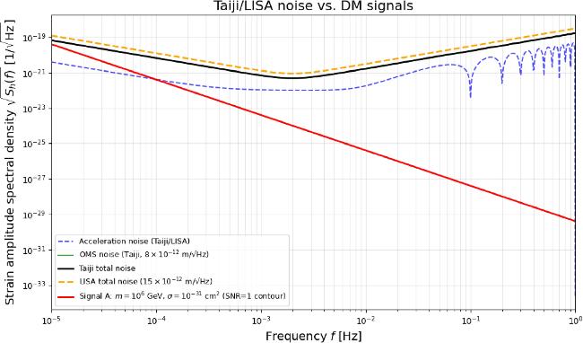
Figure 1. Power spectral density (PSD) of the test mass displacement induced by DM collisions, compared with the Taiji noise budget. The black solid line shows the total noise Taiji PSD Sn(f), decomposed into acceleration noise (ACC, shown in blue dashed line) and optical metrology system noise (OMS, shown in green solid line). The DM-induced signal PSD Sx(f) for three benchmark DM parameters: m = 106 GeV, σ = 10−35 cm2 (red), The signal follows the universal 1/f4 scaling derived in the main text. The total LISA noise is shown in yellow dashed line and shares the same acc noise with Taiji. All noise considered is one link not any TDI variables. |
Integrating equation (13 ) over the Taiji sensitivity band (10−4 Hz to 1 Hz) and setting SNR = 1 (the minimum SNR required for reliable signal detection), we derive a constraint on the product of the DM particle mass m and the DM-nucleon scattering cross-section σ. The flux of DM ΦDM is [31, 36]11 ), ρDM is the local DM density which is 0.3 GeV cm−3. Substituting equation (17 ) into the definition of event rate:
$\begin{eqnarray}{{\rm{\Phi }}}_{\rm{DM}\,}={n}_{\,\rm{DM}}\cdot \langle v\rangle =\frac{{\rho }_{\,\rm{DM}\,}}{m}\bar{v},\end{eqnarray}$
where nDM is the number density of WIMPs, $\bar{v}$ is the mean velocity of WIMPs instead of v in equation ( $\begin{eqnarray}R=\displaystyle \frac{{N}_{{\rm{A}}}}{A}{{\rm{\Phi }}}_{\,\rm{DM}}{\sigma }_{\rm{DM}\,}(A),\end{eqnarray}$
which is the number of event of per target mass and per second. NA is the Avogadro constant, A is the molar mass of the target nucleus which is golden for Taiji and σDM(A) is the cross section between a WIMP and a nucleon.Using equations (13 ) and (18 ), we do integral of SNR over frequency from 10−4 Hz to 1 Hz and it gives 20 ) is visualized in figure 2, which illustrates the trade-off between the DM particle mass and the scattering cross-section for a detectable signal in the Taiji detector under different SNR. It is important to note that the derived scaling relation mσ = constant at SNR =1 is obtained using canonical values for the local DM density ρDM = 0.3 GeV cm−3 [40] and the mean velocity $\bar{v}=220\,{\rm{km}}\,{{\rm{s}}}^{-1}$ [41], which are based on the SHM. These astrophysical parameters are subject to significant uncertainties. For instance, recent estimates of ρDM range from 0.2 to 0.6 GeV cm−3 [1, 42], while the velocity distribution may deviate from a perfect Maxwellian due to halo anisotropy [1]. Such uncertainties propagate directly into the inferred constraint on mσ, implying that the absolute bound could vary by a factor of ${ \mathcal O }(2-3)$. Nevertheless, the primary value of equation (20 ) lies not in its precise numerical prediction, but in establishing the scaling behavior between the DM mass, cross-section, and detector parameters (noise, arm length, observation time). It provides a model-agnostic benchmark for comparing the sensitivity of different experimental configurations, and demonstrates that Taiji can probe the UHDM parameter space far beyond the reach of terrestrial detectors, regardless of the exact ${ \mathcal O }(1)$ astrophysical uncertainties.
$\begin{eqnarray}\frac{N{m}^{2}\bar{{v}^{2}}}{{M}^{2}}\int {\rm{d}}f\frac{1}{{[{(2\pi f)}^{2}L]}^{2}{S}_{n}(f)}=1,\end{eqnarray}$
and the final result mσ is buried in Nm term. We choose $\bar{v}=0.0012$, observation time is T = 4 year and the mass of TM is 2 kg. All these parameters give the final result: $\begin{eqnarray}\frac{m}{1\,\rm{GeV}\,}\frac{{\sigma }_{\,\rm{DM}}}{1\,{\,\rm{cm}\,}^{2}}\approx 1{0}^{-25}.\end{eqnarray}$
The quantitative relation described by equation (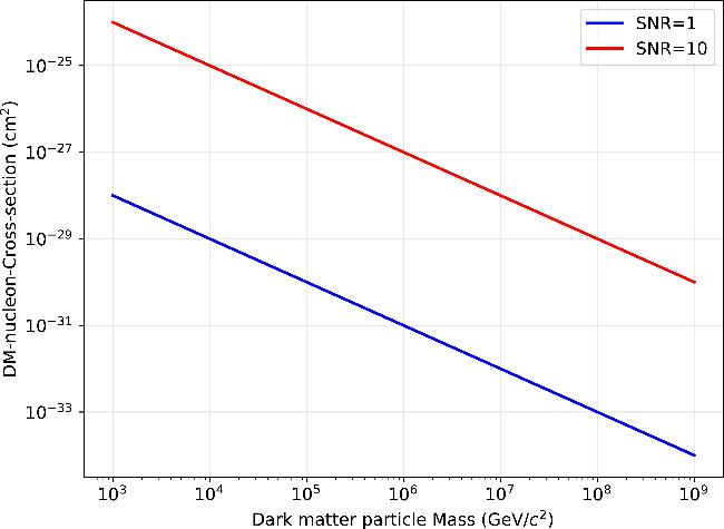
Figure 2. The constrain on the DM-nucleon cross-section σDM on Taiji. The observation time T = 4 years. The blue line represents the limit of this work under SNR = 1 and the red line is shown constrain under SNR = 10. |
Alternatively, we can propose a ‘Ideal-Taiji' detector to extract the signal caused by a WIMP collision. The noise PSD to around 10−43 1/Hz and its arm-length to be 105 m. Mass of TM is 2 kg and the molar mass of TM is 100. Note that these parameters are chosen to explore the theoretical sensitivity limit of the method, and while some exceed current engineering capabilities, they illustrate the potential gain from technological advancements (e.g. ultra-stable optics, low-noise inertial sensing) and optimized detector topology (e.g. shorter arm lengths) for DM searches. Under this ideal detector, the final result (21 ) and Taiji's result becomes and is shown in figure 1 7 , is a key feature of our scalable framework for massive DM detection.
$\begin{eqnarray}\frac{m}{1\,\rm{GeV}\,}\frac{{\sigma }_{\,\rm{DM}}}{1\,{\,\rm{cm}\,}^{2}}\approx 1{0}^{-35}.\end{eqnarray}$
It is important to clarify the nature of this ‘ideal detector'. It is not intended as a realistic engineering blueprint for Taiji, but rather as a conceptual experimental platform designed to illustrate the ultimate theoretical reach of the test-mass displacement method for UHDM detection. To construct this optimistic scenario, we have scaled the noise PSD amplitude to levels comparable to advanced ground-based detectors like aLIGO [25], and reduced the arm length to a scale similar to the ET [27, 28] (e.g. L ∼ 10 km). These parameters, while not representative of the current Taiji design, are individually technologically motivated. Our purpose is to demonstrate that, with an optimized configuration (shorter arm length to enhance SNR and lower noise), the proposed method could potentially probe cross-sections many orders of magnitude below current limits. The result in figure 3 should therefore be interpreted as a sensitivity target for future experimental concepts, rather than a forecast for the existing Taiji mission. This parametric freedom, as discussed in section 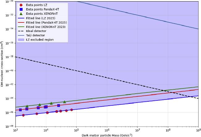


Figure 3. Projected 2σ exclusion limits on the DM-nucleon scattering cross-section σDM as a function of DM mass m, assuming an isotropic DM flux and SNR = 1 with an observation time T = 4 years. The blue solid line shows the constraint for the Taiji mission with nominal parameters. The green dashed line represents an 'ideal detector' with improved noise performance (see text for details). The shaded regions indicate parameter space already excluded by current direct detection experiments: blue is LZ 2025 [43], red is PandaX-4T [44] and green is XENONnT [13]. The scaling relation mσ = constant manifests as straight lines on this log-log plot, demonstrating that Taiji can probe a complementary parameter space in the ultra-heavy DM regime inaccessible to terrestrial experiments. |
As shown in figure 3, the projected sensitivity of this ‘ideal detector' provides stronger constraints on ultra-heavy DM compared to current experimental limits like LZ, PandaX-4T and XENONnT.
It is worth considering the impact of deviations from this Poisson assumption. If the DM flux were non-uniform in time—for instance, due to clustering of DM into dense substructures (‘clumps')—the collision events would be correlated. This would violate the independence of the phases φj, potentially leading to a different statistical distribution for the sum ${\sum }_{j}{{\rm{e}}}^{-{\rm{i}}2\pi f{t}_{j}}$. In an extreme case where collisions are perfectly correlated and occur in bursts, the effective N for a given frequency component could be reduced, and the resulting PSD might exhibit enhanced power at lower frequencies corresponding to the burst timescale. However, for a smooth and virialized Galactic DM halo described by the SHM, the Poisson assumption is the most physically motivated and widely adopted baseline model. Our analysis is therefore grounded in this standard framework.
Remark on the SNR threshold. We adopt SNR = 1 as a benchmark for sensitivity curves, following common practice in gravitational-wave astronomy [38]. However, realistic detection requires a higher threshold to control false alarms For Gaussian noise, a global false alarm probability < 0.01 over Taiji's 107 independent frequency bins necessitates an effective threshold ρth ≳ 6.5. LIGO and LISA analyses typically use SNR > 8–10 for candidate events [45–47]. Adopting ρth = 10 would shift our mσ constraints upward by a factor ${({\rho }_{{\rm{th}}}/{\rm{SNR}})}^{2}=100$ as shown in figure 2. Importantly, this rescaling does not affect the universal 1/f4 spectral shape or the scaling relation mσ = constant; our qualitative conclusions remain robust.
2.2.3. Stochastic collisions: isotropic flux case
We now generalize the analysis to the most physically relevant scenario: stochastic DM collisions with an isotropic DM flux. In this case, the direction of each DM particle's velocity relative to the TM's measurement axis is random, so we only consider the component of the impulsive force along the measurement axis. For a DM particle incident at an angle θ relative to the measurement axis (where θ is the angle between the DM velocity vector and the axis), the axial component of the impulsive force is $F(\theta ,t)=mv\cos \theta \cdot \delta (t)$, where $\cos \theta $ accounts for the projection of the total impulse onto the measurement axis. Extending this to N stochastic collisions at distinct times tj with random incident angles θj, the equation of motion for the TM (in the frequency domain) becomes: 22 ), the total frequency-domain force becomes: 24 ) into the expression for x(f) and average over the random variables αk and φk. Utilizing the orthogonality of random phases ($\langle {{\rm{e}}}^{-{\rm{i}}({\varphi }_{k}-{\varphi }_{l})}\rangle =0$ for k ≠ l) and the Rayleigh distribution property $\langle {\alpha }_{k}^{2}\rangle =2$, we find: 10 ). This modifies the constraint to a relationship of the form mσ = constant.
$\begin{eqnarray}M{(2\pi f)}^{2}x(f)=\displaystyle \sum _{j}mv\cos {\theta }_{j}\,{{\rm{e}}}^{-{\rm{i}}2\pi f{t}_{j}}.\end{eqnarray}$
To simplify the analysis of the angular dependence, we group the N collisions by their incident angle θ into infinitesimal angular intervals Δθk (k = 1, 2, …, K for large K). For an isotropic DM flux, the angular distribution function f(θ) (probability density per unit angle) is uniform over the range [0, 2π], so f(θ) = 1/(2π). The number of collisions in each angular interval Δθk is thus: $\begin{eqnarray}{\rm{\Delta }}{N}_{k}=N{\int }_{{\rm{\Delta }}{\theta }_{k}}f(\theta ){\rm{d}}\theta ,\end{eqnarray}$
For each angular subgroup k, the sum of complex exponential (accounting for random collision times) can be modeled using the same two-dimensional random walk approximation as in the unidirectional case, yielding ${\sum }_{j\in {{\rm{\Omega }}}_{k}}{{\rm{e}}}^{-{\rm{i}}2\pi f{t}_{j}}=\sqrt{{\rm{\Delta }}{N}_{k}/2}\cdot {\alpha }_{k}{{\rm{e}}}^{-{\rm{i}}{\varphi }_{k}}$, where Ωk denotes the set of collisions in the kth angular interval, αk is a standard Rayleigh variable, and φk is a uniform random phase. Substituting this into equation ( $\begin{eqnarray}F=\displaystyle \sum _{k}mv\cos {\theta }_{k}\sqrt{\frac{N{\rm{\Delta }}\theta }{4\pi }}\,{\alpha }_{k}{{\rm{e}}}^{-{\rm{i}}{\varphi }_{k}}.\end{eqnarray}$
To compute the ensemble average of the squared displacement ⟨∣x(f)∣2⟩, we substitute equation ( $\begin{eqnarray}\langle | x(f){| }^{2}\rangle ={\left(\frac{mv}{M{(2\pi f)}^{2}}\right)}^{2}\frac{N}{2},\end{eqnarray}$
which is a factor of two smaller than the aligned collision case in equation (To accurately describe this motion, we incorporate the velocity distribution of Galactic DM particles from the SHM, denoted fSHM(v) [48]. The SHM assumes a Maxwellian velocity distribution for DM particles in the Milky Way, accounting for the halo's gravitational potential and kinematic properties. Generalizing the frequency-domain displacement to account for the full range of DM velocities and isotropic incident angles, we partition the DM flux into infinitesimal velocity intervals Δv and angular intervals Δθ, leading to the displacement expression:
$\begin{eqnarray}x(f)=\frac{m}{M{(2\pi f)}^{2}}\displaystyle \sum _{k}{v}_{k}\cos {\theta }_{k}\sqrt{\frac{Nf(v){\rm{\Delta }}\theta {\rm{\Delta }}v}{4\pi }}\,{\alpha }_{k}{{\rm{e}}}^{-{\rm{i}}{\varphi }_{k}},\end{eqnarray}$
Here, vk is the characteristic velocity of the kth velocity subgroup, $\cos {\theta }_{k}$ denotes the projection of the kth subgroup's velocity onto the measurement axis, f(v) is the SHM velocity distribution function, and αk (Rayleigh-distributed) and φk (uniformly distributed) account for the stochastic nature of collision times. Averaging over all stochastic variables (amplitudes, phases, angles, and velocities), the mean squared displacement (MSD) in the frequency domain is derived as: $\begin{eqnarray}\langle | x(f){| }^{2}\rangle ={\left(\frac{m}{M{(2\pi f)}^{2}}\right)}^{2}\overline{{v}^{2}}\frac{N}{2},\end{eqnarray}$
where $\overline{{v}^{2}}$ is the second moment of the DM velocity distribution, formally defined as: $\begin{eqnarray}\overline{{v}^{2}}=\int {v}^{2}f(v){\rm{d}}v.\end{eqnarray}$
2.2.4. Stochastic collisions: anisotropic flux and the dark matter wind
The preceding analysis assumed an isotropic DM flux in the detector frame, a simplification now relaxed. The Solar System's motion through the Galactic halo introduces a preferred direction—the ‘DM wind'—which must be incorporated for accurate signal modeling.
For a space-based detector, the observer's velocity ${{\boldsymbol{v}}}_{{\rm{obs}}}$ relative to the Galactic rest frame (comprising the Solar System's orbital velocity ∼220 km s−1 and the detector's orbital motion ∼30 km s−1) transforms the Galactic-frame DM velocity distribution fgal SHM via a Galilean boost:
$\begin{eqnarray}{f}_{{\rm{\det }}}({\boldsymbol{v}})={f}_{{\rm{gal}}}({\boldsymbol{v}}+{{\boldsymbol{v}}}_{{\rm{obs}}}),\end{eqnarray}$
yielding a detector-frame distribution with a dipole moment along ${{\boldsymbol{v}}}_{{\rm{obs}}}$.Generalizing equation (27 ), the velocity vectors ${{\boldsymbol{v}}}_{j}$ are now drawn from ${f}_{{\rm{\det }}}({\boldsymbol{v}})$. For large N, the ensemble average of ∣x(f)∣2 becomes:
$\begin{eqnarray}\langle | x(f){| }^{2}\rangle ={\left(\frac{m}{M{(2\pi f)}^{2}}\right)}^{2}N\langle {v}_{\parallel }^{2}\rangle ,\end{eqnarray}$
where $\langle {v}_{\parallel }^{2}\rangle \equiv \int {({\boldsymbol{v}}\cdot \hat{n})}^{2}{f}_{{\rm{\det }}}({\boldsymbol{v}})\,{{\rm{d}}}^{3}v$ is the mean square velocity along the measurement axis $\hat{{\boldsymbol{n}}}$. The corresponding PSD is: $\begin{eqnarray}{S}_{x}(f)=\frac{{m}^{2}}{{M}^{2}{(2\pi f)}^{4}}\,R\,\langle {v}_{\parallel }^{2}\rangle .\end{eqnarray}$
Crucially, the 1/f4 dependence persists, confirming this universal spectral shape is robust against anisotropy. However, the overall amplitude now depends on detector orientation relative to the DM wind via $\langle {v}_{\parallel }^{2}\rangle $.Because ${{\boldsymbol{v}}}_{{\rm{obs}}}$ varies over the year (due to Earth's orbit), both R and $\langle {v}_{\parallel }^{2}\rangle $ acquire a time dependence, imprinting a characteristic 'annual modulation' on the signal. This provides a powerful discriminant against stationary noise sources (e.g. 1/f4 acceleration noise) that lack such temporal variation. For heliocentric detectors like LISA and Taiji, the modulation is predominantly annual; for geocentric detectors like TianQin, the orbital motion around Earth introduces additional higher-frequency modulations (periods of days).
Beyond temporal modulation, the detector's multi-channel configuration offers another discriminant. Taiji's three spacecraft and multiple interferometer arms enable cross-correlation analysis: the DM wind induces correlated displacements across different arms according to their geometric orientation relative to ${{\boldsymbol{v}}}_{{\rm{obs}}}$, whereas local instrumental noise (e.g. acceleration noise from individual TMs) is largely uncorrelated between channels. This spatial correlation pattern provides an additional handle to distinguish a genuine DM signal from stationary backgrounds. These distinct temporal and spatial signatures leave the 1/f4 spectral shape and mσ scaling relation unchanged, confirming the universal applicability of our framework while offering multiple handles for signal identification.
3. Brownian motion formalism for dark matter collisions
In this section, we develop a rigorous Brownian motion description of the TM dynamics under continuous bombardment by DM particles. This formalism is complementary to the discrete impulse model of section 2 and is particularly suitable when the collision rate is sufficiently high that the cumulative effect of many collisions can be approximated as a continuous stochastic force. The key result—the 1/f4 PSD—emerges universally, confirming the consistency of our theoretical framework across different regimes.
3.1. Langevin equation and statistical properties
Consider a TM of mass M immersed in a bath of DM particles with mass m. Each collision transfers a random momentum impulse. When the collision rate R (number of collisions per unit time per unit mass) is high, the cumulative effect can be approximated by a continuous stochastic force F(t). The equation of motion becomes the Langevin equation: 35 ):
$\begin{eqnarray}M\ddot{x}=F(t),\quad \langle F(t)\rangle =0,\end{eqnarray}$
where F(t) is the superposition of impulsive forces from individual DM-TM collisions, with vi and ti representing the relative velocity and collision time of the i-th DM particle, respectively. The statistical properties of F(t) are governed by the isotropic and homogeneous nature of the Galactic DM halo, leading to two key constraints on the DM velocity: the mean velocity is zero (no net DM flux in the Galactic rest frame), and velocities of distinct DM particles are uncorrelated. Mathematically, these properties are expressed as: $\begin{eqnarray}\langle {v}_{i}\rangle =0\quad \,\rm{and}\,\quad \langle {v}_{i}{v}_{j}\rangle =\overline{{v}^{2}}{\delta }_{ij}.\end{eqnarray}$
where δij is the Kronecker delta function (1 if i = j, 0 otherwise) and $\overline{{v}^{2}}$ is the mean squared velocity of the DM particles. Simplifying the equation of motion by introducing the TM's velocity ${v}_{M}=\dot{x}$ (time derivative of displacement), we convert the second-order differential equation to a first-order equation for vM: $\begin{eqnarray}M{\dot{v}}_{M}=F(t).\end{eqnarray}$
Integrating over time from 0 to t yields the formal solution for the TM's velocity as a function of time: $\begin{eqnarray}{v}_{M}(t)={\int }_{0}^{t}\frac{F(s)}{M}\,{\rm{d}}s.\end{eqnarray}$
Integrating the velocity once more (from 0 to t) provides the time-domain displacement of the TM, which accounts for the cumulative effect of all collisions up to time t: $\begin{eqnarray}x(t)={\int }_{0}^{t}{\int }_{0}^{u}\frac{F(s)}{M}\,{\rm{d}}s\,{\rm{d}}u.\end{eqnarray}$
Notably, the ensemble averages of both the TM's velocity and displacement vanish, i.e. ⟨vM(t)⟩ = 0 and ⟨x(t)⟩ = 0. This result follows directly from the zero-mean property of the stochastic force ⟨F(t)⟩ = 0, as the integral of a zero-mean random process over a finite interval retains a zero mean. To fully characterize the stochastic motion, we compute the second moments of the velocity and displacement, which quantify the spread of the TM's motion around the zero mean. The mean squared velocity of the TM is derived by taking the ensemble average of the square of equation ( $\begin{eqnarray}\langle {v}_{M}^{2}(t)\rangle ={\int }_{0}^{t}{\int }_{0}^{t}\frac{\langle F(s)F(u)\rangle }{{M}^{2}}\,{\rm{d}}s\,{\rm{d}}u.\end{eqnarray}$
The force autocorrelation function ⟨F(s)F(u)⟩ is derived from the Poissonian nature of DM-TM collisions, where each collision is an independent event with no temporal correlation. For a Poisson process with rate RM (total collisions per unit time), the double sum over collision events simplifies to a single sum over coincident events (since non-coincident events have uncorrelated velocities), leading to: $\begin{eqnarray}\begin{array}{rcl}\langle F(s)F(u)\rangle & = & {m}^{2}\displaystyle \sum _{i}\displaystyle \sum _{j}\langle {v}_{i}{v}_{j}\rangle \delta (s-{t}_{i})\delta (u-{t}_{j})\\ & = & {m}^{2}\overline{{v}^{2}}\displaystyle \sum _{i}\delta (s-{t}_{i})\delta (u-{t}_{i}).\end{array}\end{eqnarray}$
Evaluating the integrals, we find that the mean squared velocity depends linearly on the number of collisions N = RMT: $\begin{eqnarray}\langle {v}_{M}^{2}\rangle =N\frac{{m}^{2}}{{M}^{2}}\overline{{v}^{2}}.\end{eqnarray}$
Following a similar procedure for the displacement, we integrate the velocity autocorrelation function over time to derive the time-domain MSD of the TM: $\begin{eqnarray}\langle {x}^{2}(t)\rangle =N\frac{{m}^{2}}{2{M}^{2}}\overline{{v}^{2}}{t}^{2},\end{eqnarray}$
reflecting ballistic Brownian motion in the absence of damping.The PSD of the displacement follows directly from the force PSD via the Wiener–Khinchin theorem: A for completeness. This consistency check reinforces the robustness of our 1/f4 prediction.
$\begin{eqnarray}{S}_{x}(f)=\frac{{m}^{2}\overline{{v}^{2}}R}{M{(2\pi f)}^{4}},\end{eqnarray}$
which is identical in form to the discrete-model result. This 1/f4 scaling is therefore a universal signature, independent of the description adopted. This result exhibits a dependence on time, a hallmark of ballistic (inertial) Brownian motion—distinct from the diffusive Brownian motion observed in fluid systems—arising from the absence of significant damping in the space-based environment. Before concluding our theoretical development, we note that the time-domain description (stochastic differential equation) and the frequency-domain description (PSD) are mathematically equivalent. A detailed verification of this equivalence via the Wiener–Khinchin theorem, including the explicit derivation of the displacement autocorrelation function and its Fourier transform, is provided in Appendix 3.2. Generalization to anisotropic velocity distribution
In the preceding analysis, we assumed an isotropic DM velocity distribution for simplicity. However, in the realistic Galactic halo, the motion of the Solar System relative to the Galactic rest frame (the ‘DM wind') introduces a preferred direction in the detector frame, rendering the velocity distribution anisotropic. Moreover, the halo itself may possess net angular momentum, leading to further asymmetries. It is therefore necessary to extend the Brownian motion formalism to a general anisotropic velocity distribution ${f}_{{\rm{\det }}}({\boldsymbol{v}})$ in the detector frame and examine its impact on the signal.
3.2.1. Statistical properties of the stochastic force
For an anisotropic distribution, the velocity covariance matrix is
$\begin{eqnarray}{{\rm{\Sigma }}}_{ab}=\langle {v}_{a}{v}_{b}\rangle =\int {v}_{a}{v}_{b}\,{f}_{{\rm{\det }}}({\boldsymbol{v}})\,{{\rm{d}}}^{3}v,\end{eqnarray}$
where a, b denote spatial indices. Because different DM particles move independently (collisionless assumption), the force fluctuations from distinct particles remain uncorrelated. Consequently, the auto-correlation function of the force projected along a fixed direction, say the interferometer arm direction $\hat{e}$, can be obtained by superposing the contributions of individual particles.Let ${F}_{\parallel }(t)={\boldsymbol{F}}(t)\cdot \hat{{\boldsymbol{e}}}$ be the force component along the measurement axis. Using the same steps as in Appendix A (but focusing on the single-point auto-correlation rather than the two-point cross-correlation) and exploiting particle independence, we obtain
$\begin{eqnarray}\langle {F}_{\parallel }(t){F}_{\parallel }(t+\tau )\rangle ={m}^{2}RM\,\langle {({\boldsymbol{v}}\cdot \hat{{\boldsymbol{e}}})}^{2}\rangle \,\delta (\tau ),\end{eqnarray}$
where R is the collision rate per unit mass, and $\langle {({\boldsymbol{v}}\cdot \hat{{\boldsymbol{e}}})}^{2}\rangle $ is the mean square projection of the velocity onto the measurement axis. Compared with the isotropic case, the only change is the replacement of $\frac{1}{3}\langle {v}^{2}\rangle $ by $\langle {v}_{\parallel }^{2}\rangle $. The PSD of the force is therefore $\begin{eqnarray}{S}_{{F}_{\parallel }}(f)={m}^{2}RM\,\langle {v}_{\parallel }^{2}\rangle .\end{eqnarray}$
The displacement PSD along the measurement axis follows from the transfer function $H(f)={[M{(2\pi f)}^{2}]}^{-1}$ (neglecting weak restoring forces and damping, which are negligible in the signal band):
$\begin{eqnarray}{S}_{x}(f)=| H(f){| }^{2}{S}_{{F}_{\parallel }}(f)=\frac{{m}^{2}}{{M}^{2}{(2\pi f)}^{4}}\,R\,\langle {v}_{\parallel }^{2}\rangle .\end{eqnarray}$
Remarkably, the universal 1/f4 spectral shape remains unchanged; anisotropy only affects the overall amplitude through the factor $\langle {v}_{\parallel }^{2}\rangle $.3.2.2. Coupling to the dark matter wind and temporal modulation
In the detector frame, the velocity distribution is obtained from the Galactic rest-frame distribution fgal(v) (e.g. the SHM) by a Galilean boost:
$\begin{eqnarray}{f}_{{\rm{\det }}}({\boldsymbol{v}})={f}_{{\rm{gal}}}({\boldsymbol{v}}+{{\boldsymbol{v}}}_{{\rm{obs}}}(t)),\end{eqnarray}$
where vobs(t) is the instantaneous velocity of the detector relative to the Galactic rest frame, which includes the Solar System's peculiar motion and the detector's orbital velocity. Consequently, $\langle {v}_{\parallel }^{2}\rangle $ becomes time-dependent: $\begin{eqnarray}\langle {v}_{\parallel }^{2}(t)\rangle =\int {\left[({\boldsymbol{v}}-{{\boldsymbol{v}}}_{{\rm{obs}}}(t))\cdot \hat{{\boldsymbol{e}}}\right]}^{2}\,{f}_{{\rm{gal}}}({\boldsymbol{v}})\,{{\rm{d}}}^{3}v.\end{eqnarray}$
Expanding the square yields a constant term, a term linear in vobs (which may vanish due to symmetry of fgal), and a term quadratic in vobs. Most importantly, vobs(t) varies with the detector's orbital motion, leading to an annual modulation of $\langle {v}_{\parallel }^{2}(t)\rangle $ for heliocentric detectors (e.g. Taiji, LISA), and possibly higher-frequency modulations for geocentric detectors (e.g. TianQin). This time-dependent signature provides a powerful discriminant against stationary instrumental noise.If ${f}_{{\rm{\det }}}({\boldsymbol{v}})$ is isotropic, then $\langle {({\boldsymbol{v}}\cdot \hat{{\boldsymbol{e}}})}^{2}\rangle =\frac{1}{3}\langle {v}^{2}\rangle $, and this quantity is independent of $\hat{{\boldsymbol{e}}}$ and time. Equation (45 ) then reduces to the isotropic result derived before. Hence, the isotropic case is a special limit of the general anisotropic formalism.
4. Statistical independence of test masses and differential response
The previous analysis focused on the displacement of a single TM. However, a space-based GW interferometer measures the differential displacement between two widely separated TMs. We emphasize that while the DM wind introduces a preferred direction (anisotropy), resulting in non-zero mean forces ⟨F1⟩ and ⟨F2⟩, these are effectively constant (DC) in the detector's sensitive frequency band. The stochastic fluctuations δF1 and δF2 remain statistically independent due to the collisionless nature of cold dark matter (CDM), as proven in Appendix B . For a simple Michelson-type configuration with two TMs located at the ends of an arm of length L, the observable is δx(t) = x2(t) − x1(t), where x1(t) and x2(t) are the displacements of the two TMs along the arm direction. In this section we relate the PSD of δx(t) to that of a single TM, and examine the conditions under which the two TMs can be treated as statistically independent.
4.1. General relation for the differential PSD
For two stationary random processes x1(t) and x2(t), the PSD of their difference is
$\begin{eqnarray}{S}_{\delta x}(f)={S}_{{x}_{1}{x}_{1}}(f)+{S}_{{x}_{2}{x}_{2}}(f)-2\,{\rm{Re}}\,{S}_{{x}_{1}{x}_{2}}(f),\end{eqnarray}$
where ${S}_{{x}_{i}{x}_{i}}(f)$ is the auto PSD of xi, and ${S}_{{x}_{1}{x}_{2}}(f)$ is their cross PSD (defined via $\langle {x}_{1}^{* }(f){x}_{2}(f^{\prime} )\rangle ={S}_{{x}_{1}{x}_{2}}(f)\delta (f-f^{\prime} )$). Because the two TMs are identical and experience the same statistical environment (the DM halo and instrumental conditions), we have ${S}_{{x}_{1}{x}_{1}}(f)={S}_{{x}_{2}{x}_{2}}(f)\equiv {S}_{x}(f)$, where Sx(f) is the single-TM PSD derived in previous sections. Thus $\begin{eqnarray}{S}_{\delta x}(f)=2{S}_{x}(f)-2\,{\rm{Re}}\,{S}_{{x}_{1}{x}_{2}}(f).\end{eqnarray}$
The cross term ${S}_{{x}_{1}{x}_{2}}(f)$ encodes possible correlations between the motions of the two TMs. If the TMs are statistically independent, ${S}_{{x}_{1}{x}_{2}}(f)=0$ and the differential PSD is simply 2Sx(f). The remainder of this section is devoted to demonstrating that this independence holds for the parameter space of interest.4.2. Correlations from a single dark matter particle
One possible source of correlation is a single DM particle scattering successively off both TMs. Consider a DM particle with velocity ${\boldsymbol{v}}$ that first hits TM1 at time t, transferring a momentum ${{\boldsymbol{p}}}_{1}$ along the arm direction, and later hits TM2 at time t + τ, transferring ${{\boldsymbol{p}}}_{2}$. The time delay τ ≈ L/v∥, where v∥ is the component of ${\boldsymbol{v}}$ along the arm. For a particle to hit both TMs, its trajectory must intersect the volumes of both TMs; this requires the particle's direction to be aligned with the arm to within an angular tolerance of order $\sqrt{{A}_{{\rm{TM}}}}/L$, where ATM is the cross-sectional area of a TM perpendicular to the arm.
The joint event rate density R12(τ)—the number of pairs of hits (first on TM1, then on TM2 with delay τ) per unit time—can be estimated as
$\begin{eqnarray}{R}_{12}(\tau )\approx \frac{{A}_{{\rm{TM}}}}{4\pi {L}^{2}}\,\eta \,R,\end{eqnarray}$
where R is the single-TM collision rate and $\eta \sim { \mathcal O }(1)$ accounts for velocity distributions and finite size effects. The geometric factor ATM/(4πL2) is the probability that a particle which hit TM1 also hits TM2, assuming an isotropic velocity distribution after the first collision. Using typical parameters for Taiji (L = 3 × 10⁹ m, ATM ≈ 2.5 × 10⁻³ m2), we find $\begin{eqnarray}\frac{{A}_{{\rm{TM}}}}{4\pi {L}^{2}}\sim 2.2\times 1{0}^{-23}.\end{eqnarray}$
Even for optimistic choices of η, the correlated event rate is suppressed by more than twenty orders of magnitude relative to the single-TM hit rate. Consequently, correlations from single particles are completely negligible for ultra-heavy DM.4.3. Cross power spectral density
For a stationary Poisson process of uncorrelated hits, the force on TMi can be written as ${F}_{i}(t)={\sum }_{\alpha }{p}_{\alpha }^{(i)}\delta (t-{t}_{\alpha }^{(i)})$. The cross-correlation function of the forces is 49 ) yields
$\begin{eqnarray}\langle {F}_{1}(t){F}_{2}(t+\tau )\rangle =\int {\rm{d}}\tau ^{\prime} \,{R}_{12}(\tau ^{\prime} )\,{\langle {p}_{1}{p}_{2}\rangle }_{\tau ^{\prime} }\,\delta (\tau -\tau ^{\prime} ),\end{eqnarray}$
where ${\langle {p}_{1}{p}_{2}\rangle }_{\tau ^{\prime} }$ is the average product of the momentum transfers for a pair with delay $\tau ^{\prime} $. The cross PSD of the forces is the Fourier transform: $\begin{eqnarray}{S}_{{F}_{1}{F}_{2}}(f)=\int {\rm{d}}\tau ^{\prime} \,{R}_{12}(\tau ^{\prime} )\,{\langle {p}_{1}{p}_{2}\rangle }_{\tau ^{\prime} }\,{{\rm{e}}}^{-{\rm{i}}2\pi f\tau ^{\prime} }.\end{eqnarray}$
Because ${R}_{12}(\tau ^{\prime} )$ is proportional to the tiny geometric factor, ${S}_{{F}_{1}{F}_{2}}(f)$ is suppressed by the same factor relative to the auto PSD ${S}_{{F}_{i}{F}_{i}}(f)$. The displacement cross PSD is then obtained via the transfer function $H(f)={[M{(2\pi f)}^{2}]}^{-1}$ (neglecting damping, which is irrelevant in the signal band): $\begin{eqnarray}{S}_{{x}_{1}{x}_{2}}(f)=H{(f)}^{2}{S}_{{F}_{1}{F}_{2}}(f).\end{eqnarray}$
With the suppression factor ε ≡ (ATM/(4πL2)) η ∼ 10−22, we have $| {S}_{{x}_{1}{x}_{2}}(f)| \lesssim \epsilon \,{S}_{x}(f)$. Substituting into equation ( $\begin{eqnarray}{S}_{\delta x}(f)=2{S}_{x}(f)\left[1-{ \mathcal O }(\epsilon )\right]\approx 2{S}_{x}(f).\end{eqnarray}$
Thus, from the perspective of single-particle scattering, the two TMs are effectively independent, and the differential PSD is simply twice the single-TM PSD.4.4. Why dark matter does not behave as a coherent fluid
A more subtle concern is that even if single-particle correlations are negligible, the two TMs might still experience correlated motions if the DM behaves as a coherent fluid. In a collisional fluid, when the mean free path λ is much larger than the arm length L, the two TMs would be embedded in the same velocity field, leading to correlated motions that could cancel in the differential measurement. However, this fluid analogy does not apply to the collisionless DM that constitutes the standard cosmological model.
In the standard ΛCDM paradigm, DM particles are effectively collisionless: they interact only gravitationally, and their dynamics is governed by the Vlasov equation. Particles move independently along their trajectories, with no mechanism to exchange momentum or establish local thermodynamic equilibrium. This fundamental difference has important consequences for the correlation structure of the momentum density. For a system of independent, identically distributed particles, the two-point correlation function of the momentum density fluctuations is given by
$\begin{eqnarray}\langle \delta {\hat{p}}_{\alpha }({{\boldsymbol{x}}}_{1})\delta {\hat{p}}_{\beta }({{\boldsymbol{x}}}_{2})\rangle =n{m}^{2}\langle {v}_{\alpha }{v}_{\beta }\rangle \,\delta ({{\boldsymbol{x}}}_{1}-{{\boldsymbol{x}}}_{2}),\end{eqnarray}$
where n is the number density. This result, standard in kinetic theory for collisionless gases, shows that momentum density fluctuations at distinct spatial points are strictly uncorrelated. The Dirac delta reflects that only the same particle can contribute to both points; different particles are independent and yield zero cross-term. Hence, the velocity field of collisionless DM does not possess a continuous coherent structure on any scale. The correlation length of velocity fluctuations is zero.Consequently, the forces on two spatially separated TMs are statistically independent. The sets of particles that hit TM1 and TM2 are independent Poisson processes, and the cross PSD ${S}_{{F}_{1}{F}_{2}}(f)$ vanishes identically. This conclusion holds regardless of the value of the scattering mean free path λ = 1/(nσ) for DM-nucleon interactions; that quantity pertains to the probability of a particle scattering off a TM, not to correlations among different particles.
One might ask whether self-interacting dark matter (SIDM) [49] could alter this conclusion. In a collisional fluid, velocity correlations indeed persist over distances comparable to the self-interaction mean free path λself = 1/(nσself). However, astrophysical constraints from the Bullet Cluster, dwarf galaxy shapes, and cosmic microwave background observations limit the self-interaction cross-section to σself/m ≲ 1 cm2 g−1 [50]. For ultra-heavy DM with m ≳ 103 GeV and local density ρDM ≈ 0.3 GeV cm−3, this implies λself ≳ 1015 m, which is six orders of magnitude larger than the arm length L = 3 × 10⁹ m. Thus, for SIDM, it is not the particle model we consider here.
4.5. The mean free path and its role
The mean free path λ = 1/(nσ) for DM-nucleon scattering can be large in the ultra-heavy DM regime due to low number density or small cross section. When λ ≫ L, the probability that a given DM particle interacts with a single TM is Pint ∼ L/λ ≪ 1, and the probability of interacting with both TMs is ${P}_{{\rm{int}}}^{2}\sim {(L/\lambda )}^{2}$. This quadratic suppression is consistent with the geometric factor estimated in equation (51 ). In this regime, correlations are negligible and the TMs move independently.
Conversely, if λ ≪ L, particles interact frequently and could in principle induce correlated motions. However, such a small mean free path would require either a very high DM density or a very large cross section, which is either excluded by existing direct detection experiments for the masses we consider or lies outside the ultra-heavy DM paradigm. Our analysis thus self-consistently applies to the parameter region where λ is large and the TMs are statistically independent.
4.6. Conclusion on differential response
In summary, the differential response of a space-based interferometer preserves the characteristic 1/f4 spectral shape of the single-TM displacement, with only a factor-of-two enhancement in the PSD. The statistical independence of the two TMs follows from two complementary arguments: the geometric suppression of single-particle double hits, and—more fundamentally—the collisionless nature of DM, which ensures that momentum density fluctuations at distinct points are uncorrelated. All key conclusions of this paper—the universal 1/f4 signature, the mσ scaling relation, and the sensitivity projections—therefore remain valid for the actual detector output.
5. Experimental realities: damping and feedback
The analyses in previous sections assumed an idealized free mass. In this section, we incorporate realistic effects and quantify their impact on the DM-induced signal.
5.1. Damping and restoring forces
As introduced in equation (4 ), the TM experiences weak restoring forces (kx) and damping forces ($\gamma \dot{x}$). These originate from: 57 ) corresponds to the full equation of motion considered in [35] adapted to the space-based detector environment by including feedback forces.' The total transfer function can be written as
Gravitational gradients. From the spacecraft and nearby masses, producing an effective spring constant kgrav.
Electrostatic forces. From stray electric fields and the capacitive sensing system.
Residual gas damping. From collisions with remaining molecules in the ultra-high vacuum chamber.
Radiation pressure. From anisotropic thermal emission.
For Taiji, the drag-free control system actively cancels most disturbances, maintaining the TM in a near-inertial state. The residual acceleration noise PSD, SACC(f) implicitly includes these effects. The complete equation of motion, including feedback forces Ffb(t), is $\begin{eqnarray}M\ddot{x}+\gamma \dot{x}+kx={F}_{{\rm{DM}}}(t)+{F}_{{\rm{fb}}}(t)+{F}_{{\rm{noise}}}(t).\end{eqnarray}$
The feedback force is designed to keep the TM centered, effectively modifying the transfer function. Our equation ( $\begin{eqnarray}{H}_{{\rm{total}}}(f)=\frac{1}{M\left[{(2\pi f)}^{2}-{\omega }_{0}^{2}-{\rm{i}}(2\pi f)\gamma /M\right]+{H}_{{\rm{fb}}}^{-1}(f)},\end{eqnarray}$
where Hfb(f) represents the feedback response.5.2. Impact on DM signal
For the DM search, the key question is whether these effects distort the 1/f4 signature. For Taiji's designed performance, the DM signal PSD Sx(f) retains its 1/f4 character across the entire observational band (10−4 to 1 Hz) to within a few percent. The primary effect of damping and feedback is to introduce additional noise Fnoise(t), which is already accounted for in the total noise PSD Sn(f). The correction to the transfer function from damping and restoring forces scales as ${({f}_{0}/f)}^{2}$ and (γ/(Mf))2. For Taiji, typical values f0 ∼ 10−5 Hz and γ/M ∼ 10−8 s−1 give corrections <10−2 for f > 10−4 Hz, justifying the 1/f4 approximation to within a few percent.Therefore, our SNR calculations using the idealized transfer function remain valid as a first-order approximation. A more precise treatment requires mission-specific transfer functions and is beyond the scope of this theoretical framework.
6. A class of experiments for massive dark matter detection
The key scaling relation mσ = constant (derived for isotropic DM flux) provides a blueprint for designing a broad class of experiments to probe DM-nucleon interactions. This relation implies that for a given detector sensitivity (defined by the minimum detectable MSD), the product of the DM particle mass and scattering cross-section is constrained to a constant value—enabling targeted searches across diverse DM mass regimes (from LDM to ultra-heavy DM, UHDM). In the context of GW detectors, the output signal can be generically expressed as s(t) = n(t) + h(t), where n(t) is the detector's intrinsic noise (combining OMS noise, ACC noise, and damping-induced noise) and h(t) is the DM-induced signal (the TM's displacement). The sensitivity to h(t) is governed by the matched filtering SNR [equation (13 )], which can be enhanced through three complementary strategies:
1. Reducing the noise spectral density Sn(f). Advances in TM fabrication (e.g. ultra-smooth surfaces to minimize thermal noise) and optical metrology (e.g. phase-sensitive detection to reduce OMS noise) directly improve the SNR by lowering the background noise floor.
2. Reducing the arm length L. The SNR scales inversely with the square of the arm length L2 from equation (13 ), so detectors with shorter arm lengths are theoretically more sensitive to DM-induced displacements.
3. Extending the observation time T: The total number of DM-TM collisions N scales linearly with T, increasing the signal amplitude. Longer observation times also allow for averaging out random noise fluctuations, further boosting the SNR.
This framework is scalable to non-GW experiments as well, including dedicated DM detectors (e.g. cryogenic bolometers, nuclear recoil detectors). By optimizing the three key parameters (noise, baseline length, observation time), future experiments can probe DM parameter space well beyond the reach of current instruments—opening new windows into the nature of DM.
7. Conclusion
This work establishes a unified theoretical framework for DM detection via TM collisions in space-based GW detectors. We demonstrate that the ultra-high vacuum and microgravity environment of missions like Taiji and LISA provides a unique sensitivity to DM interactions, particularly in the ultra-heavy mass regime beyond terrestrial reach.
Our framework systematically characterizes TM motion across three regimes: idealized coherent collisions, stochastic collisions (unidirectional and isotropic), and light-DM-induced Brownian motion. A universal outcome is the 1/f4 PSD of the displacement, a distinct signature separable from GWs and instrumental noise. For the realistic isotropic Galactic DM flux, we derive a fundamental scaling relation mσ = constant at SNR = 1, offering a direct constraint on DM mass and cross-section and naturally targeting the ultra-heavy DM parameter space.
A key theoretical achievement is the rigorous unification of time- and frequency-domain descriptions via the Wiener–Khinchin theorem, confirming the mathematical consistency of the 1/f4 spectral signature. We have further demonstrated that while weak damping and restoring forces modify the TM response at very low frequencies (f ≲ 2 × 10⁻⁴ Hz), the universal 1/f4 PSD remains a robust signature of DM-induced motion across Taiji's sensitive frequency band. The framework further incorporates the SHM velocity distribution and experimental realities such as damping, providing a scalable blueprint for future detector design based on noise, arm length, and observation time.
In summary, this study positions space-based interferometers as powerful, dual-purpose instruments for both gravitational-wave astronomy and direct DM searches. Integrating DM detection into the science goals of upcoming missions like Taiji and LISA opens a new frontier in the quest to unravel the nature of DM.
Appendix A Unification of time and frequency domain descriptions
A central validation of our theoretical framework is the equivalence between time-domain and frequency-domain descriptions of DM-induced TM motion, formalized by the Wiener–Khinchin theorem [51]. This theorem establishes a one-to-one correspondence between the autocorrelation function of a stationary random process (time domain) and its PSD (frequency domain), ensuring consistency across analytical approaches [52].
A.1. Time domain: stochastic differential equation
The fundamental equation of motion for the TM in the time domain remains the stochastic differential equation describing the superposition of impulsive DM collision forces, generalized to account for the full DM velocity distribution:
$\begin{eqnarray}M\ddot{x}(t)=F(t)=\displaystyle \sum _{j=1}^{\infty }m{v}_{j}\delta (t-{t}_{j}).\end{eqnarray}$
As established earlier, F(t) is a zero-mean stationary random process (due to the homogeneity and isotropy of the Galactic DM halo). Its autocorrelation function—quantifying the correlation between the force at time t and t + τ is derived from the Poissonian collision process and the uncorrelated nature of DM velocities, yielding: $\begin{eqnarray}\langle F(t)F(t+\tau )\rangle ={m}^{2}\overline{{v}^{2}}RM\delta (\tau ),\end{eqnarray}$
where τ is the time lag, $\overline{{v}^{2}}$ is the second moment of the DM velocity distribution fSHM(v), and RM is the total collision rate. The Dirac delta function δ(τ) reflects the absence of temporal correlation between distinct collision events, a key characteristic of Poisson processes.A.2. Frequency domain: power spectral density
In the frequency domain, the TM's displacement is related to the stochastic force via the system transfer function H(f), which describes how the detector responds to forces at different frequencies. For the TM, H(f) is derived by taking the Fourier transform of the equation of motion, utilizing ${ \mathcal F }\{\ddot{x}(t)\}=-{(2\pi f)}^{2}x(f)$, leading to: A2 ), we compute SF(f) as the Fourier transform of ⟨F(t)F(t + τ)⟩:
$\begin{eqnarray}H(f)={[M{(2\pi f)}^{2}]}^{-1}.\end{eqnarray}$
The PSD of the TM's displacement Sx(f) is then the product of the squared magnitude of H(f) and the PSD of the force SF(f): $\begin{eqnarray}{S}_{x}(f)=| H(f){| }^{2}{S}_{F}(f).\end{eqnarray}$
Applying the Wiener–Khinchin theorem to the force autocorrelation function ( $\begin{eqnarray}{S}_{F}(f)={\int }_{-\infty }^{\infty }\langle F(t)F(t+\tau )\rangle {{\rm{e}}}^{-{\rm{i}}2\pi f\tau }{\rm{d}}\tau ={m}^{2}\overline{{v}^{2}}RM.\end{eqnarray}$
we derive the PSD of the TM's displacement: $\begin{eqnarray}{S}_{x}(f)=\frac{{m}^{2}\overline{{v}^{2}}R}{M{(2\pi f)}^{4}}.\end{eqnarray}$
This result retains the characteristic 1/f4 dependence observed in the low-collision-rate regime, confirming that this frequency scaling is a universal signature of DM-induced TM motion—regardless of whether collisions are sparse (stochastic) or dense (Brownian).A.3. Equivalence of approaches
To verify consistency, we relate the frequency-domain MSD to the time-domain MSD [equation (40 )]. The frequency-domain MSD is ⟨∣x(f)∣2⟩ = Sx(f)T, where T is the observation time. Substituting equation (A6 ) and N = RMT (total collisions over T) into this relation yields: 40 ) when converted to the frequency domain. This equivalence confirms that time-domain stochastic calculus and frequency-domain random process theory provide complementary, mathematically consistent descriptions of DM-induced TM motion—strengthening the reliability of our derived constraints on DM properties.
$\begin{eqnarray}\langle | x(f){| }^{2}\rangle ={\left(\frac{m\sqrt{\overline{{v}^{2}}}}{M{(2\pi f)}^{2}}\right)}^{2}\frac{RMT}{2}.\end{eqnarray}$
This expression is identical to the frequency-domain MSD derived from the random phase sum model and consistent with the time-domain MSD (A.4. Equivalence of approaches: detailed verification
We now rigorously demonstrate the equivalence between the time-domain and frequency-domain descriptions by computing the time-averaged autocorrelation function of the TM's displacement and its Fourier transform. Starting from the time-domain expression for the displacement autocorrelation function derived from stochastic calculus, we have for τ ≥ 0:
$\begin{eqnarray}\langle x(t)x(t+\tau )\rangle =\frac{{m}^{2}{v}^{2}R}{6M}\left(3{t}^{2}\tau +3t{\tau }^{2}+{\tau }^{3}\right).\end{eqnarray}$
This result is obtained by integrating the velocity autocorrelation function $\langle {v}_{M}(s){v}_{M}(u)\rangle =\frac{{m}^{2}{v}^{2}R}{M}\min (s,u)$ over the appropriate time intervals.For a finite observation time T, we define the time-averaged autocorrelation function as: A9 ) and performing the integration yields:
$\begin{eqnarray}{\bar{R}}_{x}(\tau )=\frac{1}{T}{\int }_{0}^{T}\langle x(t)x(t+\tau )\rangle \,{\rm{d}}t.\end{eqnarray}$
Substituting equation ( $\begin{eqnarray}{\bar{R}}_{x}(\tau )=\frac{{m}^{2}{v}^{2}R}{6M}\left({T}^{2}\tau +\frac{3}{2}T{\tau }^{2}+\frac{1}{3}{\tau }^{3}\right).\end{eqnarray}$
In the limit of large T (i.e. T ≫ τ), the dominant term is proportional to T2τ: $\begin{eqnarray}{\bar{R}}_{x}(\tau )\approx \frac{{m}^{2}{v}^{2}R}{6M}{T}^{2}\tau .\end{eqnarray}$
The PSD of the displacement is then obtained via the Fourier transform of ${\bar{R}}_{x}(\tau )$:
$\begin{eqnarray}{S}_{x}(f)={\int }_{-\infty }^{\infty }{\bar{R}}_{x}(\tau ){{\rm{e}}}^{-{\rm{i}}2\pi f\tau }\,{\rm{d}}\tau .\end{eqnarray}$
Substituting the approximate expression above and evaluating the integral: $\begin{eqnarray}\begin{array}{rcl}{S}_{x}(f) & \approx & \frac{{m}^{2}{v}^{2}R}{6M}{T}^{2}{\displaystyle \int }_{-\infty }^{\infty }\tau {{\rm{e}}}^{-{\rm{i}}2\pi f\tau }\,{\rm{d}}\tau \\ & = & \frac{{m}^{2}{v}^{2}R}{6M}{T}^{2}\cdot \frac{1}{{(2\pi f)}^{2}}{\left[\tau {{\rm{e}}}^{-{\rm{i}}2\pi f\tau }\right]}_{-\infty }^{\infty }\\ & & -\frac{{m}^{2}{v}^{2}R}{6M}{T}^{2}\cdot \frac{1}{{(2\pi f)}^{2}}{\displaystyle \int }_{-\infty }^{\infty }{{\rm{e}}}^{-{\rm{i}}2\pi f\tau }{\rm{d}}\tau .\end{array}\end{eqnarray}$
The first term vanishes under appropriate boundary conditions, and the second term gives a Dirac delta function at f = 0, which is excluded for f > 0. More rigorously, retaining all terms in equation (A13 ) and performing the full Fourier transform yields: A6 ). Thus, the time-domain and frequency-domain descriptions are mathematically equivalent, confirming the consistency of our theoretical framework. This equivalence reinforces that the 1/f4 PSD is a universal and robust signature of DM-induced TM motion, independent of the specific analytical approach.
$\begin{eqnarray}{S}_{x}(f)=\frac{{m}^{2}{v}^{2}R}{M{(2\pi f)}^{4}}\left[1-\frac{3}{2\pi fT}+{ \mathcal O }\left(\frac{1}{{(fT)}^{2}}\right)\right].\end{eqnarray}$
In the long-observation time limit (f ≫ 1/T), which is the relevant regime for experimental observations, this simplifies to: $\begin{eqnarray}{S}_{x}(f)\approx \frac{{m}^{2}{v}^{2}R}{M{(2\pi f)}^{4}}.\end{eqnarray}$
Noting that ${v}^{2}=\overline{{v}^{2}}$ (the second moment of the DM velocity distribution), this result is identical to the frequency-domain PSD derived in equation (Appendix B Statistical independence of forces in collisionless dark matter
This appendix establishes the rigorous statistical foundation for treating two spatially separated TMs as independent detectors. We prove that in the standard collisionless CDM paradigm, the fluctuating components of the stochastic forces at distinct spatial points have strictly vanishing cross-correlations, regardless of whether the velocity distribution is isotropic or anisotropic (e.g. due to the DM wind).
B.1. Factorization theorem for non-interacting systems
The CDM model describes particles that interact only via a smooth external gravitational potential φext(r), with no particle-particle collisions. The N-particle Hamiltonian separates additively:
$\begin{eqnarray}{H}_{N}=\displaystyle \sum _{i=1}^{N}\left[\frac{| {{\boldsymbol{p}}}_{i}{| }^{2}}{2m}+m{\phi }_{\,\rm{ext}\,}({{\boldsymbol{r}}}_{i})\right]\equiv \displaystyle \sum _{i=1}^{N}h({{\boldsymbol{x}}}_{i}),\end{eqnarray}$
where xi = (ri, pi) denotes the phase-space coordinates of particle i.The Liouville equation governing the N-particle distribution function FN(x1, …, xN, t) reads:
$\begin{eqnarray}\frac{\partial {F}_{N}}{\partial t}=\{{H}_{N},{F}_{N}\}=\displaystyle \sum _{i=1}^{N}{\{h({{\boldsymbol{x}}}_{i}),{F}_{N}\}}_{i}.\end{eqnarray}$
The subscript i indicates that the Poisson bracket acts only on the variables of particle i.Theorem: If the initial distribution factorizes as ${F}_{N}({{\boldsymbol{x}}}_{1},\ldots ,\,{{\boldsymbol{x}}}_{N},0)={\prod }_{i=1}^{N}{f}_{1}({{\boldsymbol{x}}}_{i},0)$, the exact solution at any time t maintains the product structure:
$\begin{eqnarray}{F}_{N}({{\boldsymbol{x}}}_{1},\,\ldots ,\,{{\boldsymbol{x}}}_{N},t)=\displaystyle \prod _{i=1}^{N}{f}_{1}({{\boldsymbol{x}}}_{i},t),\end{eqnarray}$
where each single-particle distribution f1 evolves according to the Vlasov equation: $\begin{eqnarray}\frac{\partial {f}_{1}}{\partial t}+\frac{{\boldsymbol{p}}}{m}\cdot {{\rm{\nabla }}}_{{\boldsymbol{r}}}{f}_{1}-{{\rm{\nabla }}}_{{\boldsymbol{r}}}{\phi }_{\,\rm{ext}\,}\cdot {{\rm{\nabla }}}_{{\boldsymbol{p}}}{f}_{1}=0.\end{eqnarray}$
Proof. Substituting the product form into equation (B2 ) yields: B4 ) for each particle. Uniqueness of solutions to the Liouville equation guarantees this is the only solution.
$\begin{eqnarray}\displaystyle \sum _{i=1}^{N}{\left(\frac{\partial {f}_{1}}{\partial t}\right)}_{i}\displaystyle \prod _{j\ne i}{f}_{1}({{\boldsymbol{x}}}_{j})=\displaystyle \sum _{i=1}^{N}{\{h({{\boldsymbol{x}}}_{i}),{f}_{1}({{\boldsymbol{x}}}_{i})\}}_{i}\displaystyle \prod _{j\ne i}{f}_{1}({{\boldsymbol{x}}}_{j}).\end{eqnarray}$
Since each term in the sum depends only on distinct variables, equality holds term-by-term, reducing to equation (The factorization theorem implies that particle trajectories remain statistically independent for all time. In the context of kinetic theory, CDM constitutes a Vlasov gas rather than a Boltzmann gas; the absence of collisional interactions preserves the product structure of the phase-space distribution exactly.
B.2. Vanishing cross-correlations of fluctuations at spatial separation
Consider two TMs located at positions r1 and r2 with separation L = ∣r2 − r1∣ ∼ 3 × 10⁹ m. The instantaneous force on TM a (a = 1, 2) can be decomposed into a mean (DC) component and a fluctuating (AC) component:
$\begin{eqnarray}{{\boldsymbol{F}}}_{a}(t)=\mathop{\underbrace{\langle {{\boldsymbol{F}}}_{a}\rangle }}\limits_{\,\rm{dark matter wind}\,}+\mathop{\underbrace{\delta {{\boldsymbol{F}}}_{a}(t)}}\limits_{\,\rm{stochastic fluctuations}\,},\end{eqnarray}$
where ⟨Fa⟩ is the time-independent mean force arising from the bulk motion of the Solar System through the Galactic halo (non-zero for anisotropic velocity distributions), and δFa(t) = Fa(t) − ⟨Fa⟩ represents the zero-mean stochastic fluctuations due to individual particle collisions.Due to the factorization theorem, the joint probability distribution of particles in regions Ω1 (surrounding r1) and Ω2 (surrounding r2) separates:
$\begin{eqnarray}\begin{array}{l}{F}_{{N}_{1}+{N}_{2}}({\{{{\boldsymbol{x}}}_{i}\}}_{i\in {{ \mathcal I }}_{1}},{\{{{\boldsymbol{x}}}_{j}\}}_{j\in {{ \mathcal I }}_{2}},t)={F}_{{N}_{1}}({\{{{\boldsymbol{x}}}_{i}\}}_{i\in {{ \mathcal I }}_{1}},t)\\ \cdot {F}_{{N}_{2}}({\{{{\boldsymbol{x}}}_{j}\}}_{j\in {{ \mathcal I }}_{2}},t),\end{array}\end{eqnarray}$
where ${{ \mathcal I }}_{a}$ denotes the index set of particles in region Ωa. This factorization ensures that the fluctuations δF1 and δF2 are statistically independent stochastic processes.The covariance (cross-correlation of fluctuations) is defined as:
$\begin{eqnarray}\begin{array}{l}\langle \delta {F}_{1,a}(t)\delta {F}_{2,b}(t+\tau )\rangle \equiv \langle [{F}_{1,a}(t)-\langle {F}_{1,a}\rangle ]\left[{F}_{2,b}(t+\tau )\right.\\ \left.-\langle {F}_{2,b}\rangle \right]\rangle .\end{array}\end{eqnarray}$
Expanding using the force expression equation (B6 ) and applying the factorization property equation (B7 ):
$\begin{eqnarray}\begin{array}{l}\langle \delta {F}_{1,a}(t)\delta {F}_{2,b}(t+\tau )\rangle \\ \,=\,\langle {F}_{1,a}(t){F}_{2,b}(t+\tau )\rangle -\langle {F}_{1,a}\rangle \langle {F}_{2,b}\rangle \\ \,=\,{m}^{2}\displaystyle \sum _{i\in {{ \mathcal I }}_{1}}\displaystyle \sum _{j\in {{ \mathcal I }}_{2}}\langle {v}_{i,a}(t){\delta }^{(3)}({{\boldsymbol{r}}}_{1}-{{\boldsymbol{r}}}_{i}(t))\rangle \\ \,\times \,\langle {v}_{j,b}(t+\tau ){\delta }^{(3)}({{\boldsymbol{r}}}_{2}-{{\boldsymbol{r}}}_{j}(t+\tau ))\rangle \\ \,-\,\langle {F}_{1,a}\rangle \langle {F}_{2,b}\rangle \\ \,=\,\langle {F}_{1,a}\rangle \langle {F}_{2,b}\rangle -\langle {F}_{1,a}\rangle \langle {F}_{2,b}\rangle =0.\end{array}\end{eqnarray}$
Thus we obtain the exact result for the fluctuating components:
$\begin{eqnarray}\,\begin{array}{||}\hline \langle \delta {F}_{1,a}(t)\delta {F}_{2,b}(t+\tau )\rangle =0,\quad \forall {{\boldsymbol{r}}}_{1}\ne {{\boldsymbol{r}}}_{2},\forall \tau .\\ \hline\end{array}\,\end{eqnarray}$
DC offset and differential measurement. The mean forces ⟨F1⟩ and ⟨F2⟩ may be non-zero and correlated (both determined by the common DM wind for anisotropic distributions), but they are constant in time, varying only on the orbital timescale (∼year, f ∼ 10−8 Hz). In the frequency domain, they contribute only to the zero-frequency bin. In the differential displacement measurement δx = x2 − x1, these DC components either cancel exactly (for identical TM materials) or appear as constant biases (for differential material coupling), neither of which affects the stochastic 1/f4 signal power in the sensitive band 10−4–1 Hz.
The cross-PSD of the fluctuations therefore vanishes:
$\begin{eqnarray}{S}_{\delta {F}_{1}\delta {F}_{2}}(f)={ \mathcal F }[\langle \delta {F}_{1,a}\delta {F}_{2,b}\rangle ]=0\quad \,\rm{for all}\,f\ne 0.\end{eqnarray}$
Consequently, the differential displacement PSD is exactly twice the single-test-mass PSD of the fluctuating component:
$\begin{eqnarray}{S}_{\delta x}(f)=2{S}_{\delta x}^{(1)}(f),\end{eqnarray}$
preserving the universal 1/f4 spectral shape.B.3. Distinction from collisional fluids
The vanishing of cross-correlations in CDM contrasts sharply with collisional fluids. In a fluid described by the Boltzmann equation, particle collisions establish velocity correlations over the mean free path $\lambda ={(n{\sigma }_{\,\rm{self}\,})}^{-1}$. When λ ≫ L, hydrodynamic fluctuations at two points separated by distance L remain correlated, leading to non-vanishing covariance of fluctuations.
However, CDM is collisionless: σself → 0 and λ → ∞. The Vlasov equation (B4 ) lacks the collision integral that correlates particle velocities. Consequently, the two-point correlation function of the momentum density fluctuations satisfies:
$\begin{eqnarray}\langle \delta {p}_{a}({{\boldsymbol{r}}}_{1},t)\delta {p}_{b}({{\boldsymbol{r}}}_{2},t)\rangle \propto {\delta }^{(3)}({{\boldsymbol{r}}}_{1}-{{\boldsymbol{r}}}_{2}),\end{eqnarray}$
exhibiting zero correlation length. The Dirac delta structure reflects that only the same particle can contribute to both points; distinct particles are statistically orthogonal, regardless of the mean velocity (wind) of the halo.Thus, the fluid analogy—often invoked to argue that large mean free paths imply correlated motion—is mathematically invalid for CDM. The proper kinetic treatment reveals that spatially separated TMs experience genuinely independent stochastic fluctuations, validating the differential measurement strategy employed in the main text.