

1. Introduction
Understanding critical phenomena has been one of the central topics in condensed matter physics for decades. In recent years, intensive efforts have been devoted to investigations on continuous phase transitions beyond the Landau–Ginzburg–Wilson (LGW) paradigm. A typical example is the deconfined quantum criticality, which describes the putative continuous phase transition between two ordered phases with incompatible broken symmetry [1–15]. Furthermore, although the deconfined quantum criticality was originally proposed in quantum phase transitions, it was shown that it also has its classical counterparts [16–21].
The classical dimer model is one of the typical models which hosts such unconventional phase transitions [22–27]. In two dimensions, the dimer model on bipartite lattice undergoes the Kosterlitz–Thouless transition from a columnar phase at low temperatures to a disordered critical phase at high temperatures [28–32]. In contrast, the three-dimensional (3D) bipartite lattice dimer model exhibits a different type of phase transition. Although the system also evolves from a disordered phase at high temperatures to a columnar ordered phase at low temperatures, the transition in 3D is continuous and cannot be described by the framework of conventional LGW theory [27, 33, 34].
It was shown that the phase transition in 3D dimer model can be characterized by a field theory that features two complex matter fields coupled to a non-compact U(1) gauge field [17–21]. In addition, it has been demonstrated that the transition in the 3D cubic dimer model exhibits an emergent SO(5) symmetry at criticality [35]. In addition, critical exponents obtained from numerical simulations do not match those of conventional LGW universality class [27, 34].
These intriguing properties have meant that this model has attracted extensive research attention. However, previous studies mainly focus on the equilibrium properties of this model [34, 36, 37]. While nonequilibrium critical dynamics have been explored in certain quantum systems, which share the similar effective field theory [38, 39], the nonequilibrium properties for the classical dimer models remain largely unknown.
Among the diverse forms of nonequilibrium processes, relaxation dynamics stand out as a representative prototype [40–52]. It was shown that universal dynamic scaling behaviors not only appear in the long-time stage [53, 54], but also emerge in the short-time stage [40, 41], characterized by the critical initial slip exponent θ, in addition to the usual dynamic exponent z. In usual classical systems, θ is positive [40]. Furthermore, short-time dynamics offers a high-efficiency strategy for extracting critical points and critical exponents without equilibrating the system, thus conserving computational resources while circumventing the impacts of critical slowing down [40–52]. In addition, the short-time dynamics were generalized to the quantum phase transitions [38, 55–65]. However, to the best of our knowledge, the dynamic critical exponent z and the critical initial slip exponent θ have not been determined for the 3D classical dimer model in previous studies.
Given the significance of the dimer model and the universality of relaxation critical dynamics, investigations into the relaxation dynamics of phase transitions in the dimer model are imperatively required. In this paper, we explore the short-time dynamics of the 3D classical cubic dimer model starting from both ordered and disordered initial states via the Monte Carlo simulation. By focusing on short-time dynamics of the square of the order parameter component ${N}_{x}^{2}$ for different initial states, we retrieve both the critical temperature Tc and the static critical exponent β/ν, which agree well with equilibrium finite-size scaling results; additionally, we successfully derive the dynamic critical exponent z = 1.92(1). Moreover, we also determine the critical initial slip exponent θ from the time-correlation function Q(t) of the order parameter starting from disordered initial states. Remarkably, we find that θ is negative here, in sharp contrast to the usual cases in which θ is positive. We attribute this to the emergent symmetry or the local constraint induced by the Gauss law at the critical point of this model.
The remainder of this paper is organized as follows. In section 2 , we introduce the classical cubic dimer model and the relevant observables, and describe the algorithm for the study. In section 3 , we briefly review the short-time dynamic scaling and show the expected scaling relations for ordered and disordered initial conditions. The numerical results for the short-time dynamics are presented and analyzed in section 4 , where the critical temperature and the critical exponents are determined through scaling analyses. Finally, section 5 is devoted to a summary of our main results.
2. Model and numerical method
The dimer model studied here is defined on a cubic lattice of linear size L (total number of sites N = L3), where the lattice links are occupied by hard-core dimers. By defining ${d}_{\mu }(\overrightarrow{r})\in [0,1]$ as the occupation number between the site $\overrightarrow{r}$ and $\overrightarrow{r}+{\overrightarrow{\delta }}_{\mu }$ (${\overrightarrow{\delta }}_{\mu }$ is a unit vector in μ-direction), the number of dimers at the site $\overrightarrow{r}$ is given by $n(\overrightarrow{r})={\sum }_{\mu }\left[{d}_{\mu }(\overrightarrow{r})+{d}_{\mu }(\overrightarrow{r}-{\overrightarrow{\delta }}_{\mu })\right]$. Only dimer configurations ${ \mathcal C }$ that obey the closed-packing condition $n(\overrightarrow{r})=1$, i.e., one dimer per site, contribute to the partition function.
The partition function is defined as ${ \mathcal Z }\equiv {\sum }_{{ \mathcal C }}{{\rm{e}}}^{-\beta {E}_{{ \mathcal C }}}$, wherein the energy of an allowed configuration ${ \mathcal C }$ is given by [34]
$\begin{eqnarray}\begin{array}{r}{E}_{{ \mathcal C }}={v}_{2}{N}_{2}+{v}_{4}{N}_{4},\end{array}\end{eqnarray}$
where N2 is the number of plaquettes of the lattice that contain two parallel dimers, and N4 is the number of unit cubes sustaining four parallel dimers, both illustrated in figures 1(a)–(b).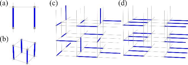
Figure 1. Two types of interactions and two types of initial states in the dimer model. (a) Two parallel dimers on the plane contribute energy v2. (b) Four parallel dimers on a unit cube contribute energy v4. In this study, we fixed v2 = − 1 and v4 = 10. (c) The disordered initial state with Nx = 0, typical of a Coulomb phase. (d) The completely ordered initial state with Nx = 1, representing a columnar phase. |
In this study, we restrict ourselves to the case of attractive plaquette interactions v2 while the cubic interaction v4 is repulsive. We focus on the strongly frustrated condition to avoid any crossover effects [34]. In the remainder of this study, we set v2 = − 1 and v4 = 10 which are the same as a set of parameters in [34]. Therefore, the results obtained in the following contents will also be compared with those in [34].
The system undergoes a continuous transition from the disordered Coulomb phase to the ordered phase [34]. At the critical point, an emergent SO(5) symmetry appears and the order parameter has five equivalent components [35]. In this work, we focus on a single component Nx of the order parameter. Here Nx denotes the thermal-averaged x-component of the order parameter, defined as
$\begin{eqnarray}{N}_{x}\equiv \frac{2}{{L}^{d}}\left\langle \displaystyle \sum _{\overrightarrow{r}}{(-1)}^{{r}_{x}}{d}_{x}(\overrightarrow{r})\right\rangle ,\end{eqnarray}$
where rx is the x-component of $\overrightarrow{r}$ and ⟨ ⋯ ⟩ represents the thermal average. In the thermodynamic limit, Nx is zero in the disordered Coulomb phase and nonzero in the columnar ordered phase.Since the order parameter Nx averages to zero in finite-size systems, critical properties cannot be directly extracted from Nx. It is therefore convenient to consider the square of the order parameter, defined as
$\begin{eqnarray}{N}_{x}^{2}\equiv \frac{4}{{L}^{2d}}\left\langle {\left(\displaystyle \sum _{\overrightarrow{r}}{(-1)}^{{r}_{x}}{d}_{x}(\overrightarrow{r})\right)}^{2}\right\rangle .\end{eqnarray}$
By analyzing the short-time scaling behavior of ${N}_{x}^{2}$, one can obtain both static critical exponent β/ν and dynamic critical exponent z [45, 46].Moreover, the short-time critical dynamics shows that the time-correlation function contains additional information about the universal critical initial slip in the early-time stage [40]. The critical initial slip behavior is characterized by the critical initial exponent θ, which can be readily obtained via the total time-correlation of the order parameter, Q(t), proposed in [49]. Specifically, here Q(t) reads
$\begin{eqnarray}Q(t)\equiv \frac{2}{{L}^{d}}\left\langle \left(\displaystyle \sum _{\overrightarrow{r}}\displaystyle \sum _{\overrightarrow{r}^{\prime} }{(-1)}^{{r}_{x}+{r}_{x}^{{\prime} }}{d}_{x}(\overrightarrow{r},t){d}_{x}(\overrightarrow{r}^{\prime} ,0)\right)\right\rangle .\end{eqnarray}$
We employ the standard Metropolis algorithm [66, 67] with local updates to simulate the nonequilibrium dynamics. It has been established that the Metropolis Monte Carlo dynamics falls within the Model A universality class, and is straightforward to implement in experiments [53, 54]. Specifically, we randomly select a plaquette containing two parallel dimers, as illustrated in figure 1(a), and update the configuration by flipping these dimers to the two adjacent links that are initially unoccupied. The time unit is defined as a Monte Carlo sweep through the lattice.
We study the nonequilibrium short-time dynamics from both the disordered initial state and the completely ordered initial state. Both initial states are illustrated in figures 1(c)–(d). The ordered state is prepared straightforwardly by placing the dimers on alternating links along the x axis, as shown in figure 1(d). The disordered initial states are obtained by evolving this ordered configuration at a sufficiently high temperature until the order parameter vanishes and becomes stationary. In this way, both initial states belong to the same topological sector [26].
3. Scaling for the short-time dynamics
In addition to the universal behavior in the long-time regime [53, 68], systems near criticality can exhibit universal relaxation dynamics in the macroscopic short-time stage, which sets in immediately after a microscopic timescale tmic [40]. It was shown that starting from an uncorrelated state with initial order parameter m0, the scale transformation of a macroscopic observable O is given by [40, 47],
$\begin{eqnarray}O(t,\tau ,L,{N}_{x0})={b}^{-x}O({b}^{-z}t,\ {b}^{1/\nu }\tau ,\ {b}^{-1}L,\ {b}^{{x}_{0}}{N}_{x0}),\end{eqnarray}$
in which b is the rescaling factor, t denotes the relaxation time, τ is the reduced temperature, L is the linear system size, x is the scaling dimension of O, ν is the correlation length exponent, z is the dynamic critical exponent, and x0 is the dimension of the initial order parameter Nx0 and satisfies x0 = θz + β/ν. For instance, the square of the order parameter ${N}_{x}^{2}$ changes as [40, 47], $\begin{eqnarray}{N}_{x}^{2}(t,\tau ,L,{m}_{0})={b}^{-2\beta /\nu }{N}_{x}^{2}({b}^{-z}t,\ {b}^{1/\nu }\tau ,\ {b}^{-1}L,\ {b}^{{x}_{0}}{N}_{x0}),\end{eqnarray}$
under scale transformation with the rescaling factor b.For the uncorrelated disordered initial state, Nx0 = 0, which corresponds to the disordered fixed point of Nx0, the dynamic scaling form of ${N}_{x}^{2}$ at the critical point follows by setting the rescaling factor b = L in equation (6 ) [40, 47],
$\begin{eqnarray}{N}_{x}^{2}(t,L)={L}^{-2\beta /\nu }{f}_{{N}_{x}}\left(t{L}^{-z}\right),\end{eqnarray}$
in which ${f}_{{N}_{x}}$ is the scaling function.In the short-time regime, the correlation length is smaller than the system size. Accordingly, the definition of ${N}_{x}^{2}$ in equation (3 ) indicates that ${N}_{x}^{2}\propto {L}^{-d}$. In this situation, the scaling function ${f}_{{N}_{x}}$ should satisfy [69], 8 ) and (7 ), the fact that ${N}_{x}^{2}\propto {L}^{-d}$ requires that,
$\begin{eqnarray}{f}_{{N}_{x}}(t{L}^{-z})\propto {(t{L}^{-z})}^{\kappa }.\end{eqnarray}$
Combining equations ( $\begin{eqnarray}\kappa =(d-2\beta /\nu )/z,\end{eqnarray}$
leading to the short-time power-law scaling behavior [41, 46, 69], $\begin{eqnarray}{N}_{x}^{2}(t,L)\propto {L}^{-d}\,{t}^{(d-2\beta /\nu )/z}.\end{eqnarray}$
In addition, for the disordered initial state with Nx0 = 0, at the critical point τ = 0, the time-correlation function Q obeys the dynamic finite-size scaling form [49], 11 ) reduces to a power-law scaling relation [49],
$\begin{eqnarray}Q(t,L)={L}^{\theta z}\,{f}_{Q}\left(t{L}^{-z}\right),\end{eqnarray}$
in which fQ is also the scaling function. In the short-time stage t ≪ Lz, the correlation length is far smaller than the system size; accordingly, Q(t) is expected to be size-independent. In this way, equation ( $\begin{eqnarray}Q(t)\propto {t}^{\theta }.\end{eqnarray}$
For the completely ordered initial state, in which Nx0 = 1, corresponding to the ordered fixed point of Nx0, in the short-time regime and for sufficiently large system sizes, ${N}_{x}^{2}$ exhibits a power-law decay [40, 47, 50],
$\begin{eqnarray}{N}_{x}^{2}(t)\propto {t}^{-2\beta /\nu z},\end{eqnarray}$
which is independent of L since the correlation length is much smaller than L.For notational convenience, in the following discussion we denote the order parameter ${N}_{x}^{2}$ by ${N}_{d}^{2}$ for disordered initial conditions and by ${N}_{o}^{2}$ for ordered initial conditions.
4. Short-time dynamics in the classical dimer model
First, we locate the critical temperature Tc via the short-time dynamics. From the scaling relation (10 ), at Tc, ${N}_{d}^{2}(t)$ should evolve obeying a power function of the time [43, 52]; while away from the critical point, ${N}_{d}^{2}(t)$ will deviate from the power function. This demonstrates the feasibility of determining the critical point from the short-time dynamics of ${N}_{d}^{2}(t)$.
In practice, the critical point is determined by searching for the minimum squared deviation of the slope of the curves of ${N}_{x}^{2}$ versus t in log-log coordinates for different temperatures. Here, the system size is chosen as L = 100, for which we have confirmed the effect of finite size on the position of the critical point can be ignored. The simulations are carried out with five temperatures T = 0.660, 0.666, 0.672, 0.678 and 0.684 as shown in figure 2. Data within the microscopic timescale tmic, which are dependent on microscopic details, are not included. The values of ${N}_{d}^{2}(t)$ at temperatures between T = 0.660 and 0.684 are obtained by quadratic interpolation. Based on these interpolated data, the slopes of ${N}_{d}^{2}$ as a function of time t are fitted for different temperatures. Specifically, for each temperature, data for ${N}_{d}^{2}$ in the time interval between 2 × 10⁴ and 2 × 10⁵ are partitioned into four subintervals, from which local slopes are extracted. The squared deviation of these slopes in subintervals from their averaged value is then calculated to quantify the deviation from a power-law behavior. In the inset of figure 2, the squared deviation is shown for different temperatures. The minimum position in this plot yields that the critical point is near T = 0.672. To estimate the statistical error of the critical temperature Tc, we first fit the curve of ${N}_{d}^{2}$ versus t in the range t ∈ [2 × 10⁴, 2 × 10⁵] at T = 0.672, i.e., the solid line in the main plot of figure 2. Then we perform fitting on the interpolated data for different temperatures around T = 0.672 over the same time range and the minimum deviation of the temperature at which the fitted slope falls outside the error range of the slope for T = 0.672 provides an estimate of the error. Accordingly, we obtain Tc = 0.672(1). This value is consistent with those reported in previous studies, Tc = 0.6718(2) [35] and 0.672(1) [34], wherein the usual equilibrium finite-size scaling methods were employed.
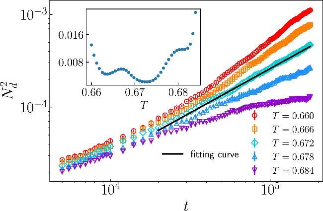
Figure 2. Estimation of the critical point of the 3D dimer model. The time evolution of ${N}_{d}^{2}(t)$ starting from the disordered state for different temperatures. The solid line shows the power-law fit of ${N}_{d}^{2}(t)$ versus t in the time range t ∈ [2 × 10⁴, 2 × 10⁵] at Tc = 0.672. The inset displays the squared deviation of ${N}_{d}^{2}(t)$ from the power-law behavior. The system size is chosen as L = 100. Log-log coordinates are used for the main figure. |
Then we determine the dynamic exponent z. We consider the evolution of the ratio ${N}_{d}^{2}/{N}_{o}^{2}$ [70, 71]. According to the scaling relations (10 ) and (13 ) for ${N}_{d}^{2}$ and ${N}_{o}^{2}$, respectively, in the short-time scaling range, ${N}_{d}^{2}/{N}_{o}^{2}$ should satisfy ${N}_{d}^{2}/{N}_{o}^{2}\propto {t}^{d/z}$ [70, 71]. Figure 3 shows the numerical results of ${N}_{d}^{2}/{N}_{o}^{2}$ in the time range t ∈ [2 × 10⁴, 2 × 10⁵] at Tc = 0.672. The power fit gives d/z = 1.56(1). Substituting d = 3, we obtain the dynamic critical exponent as z = 1.92(1). For comparison, in the 3D Ising model with Model A dynamics the dynamic exponent is typically reported as z = 2.04(3) [72]. The smaller value obtained here may be related to the local constraint in the dimer model.
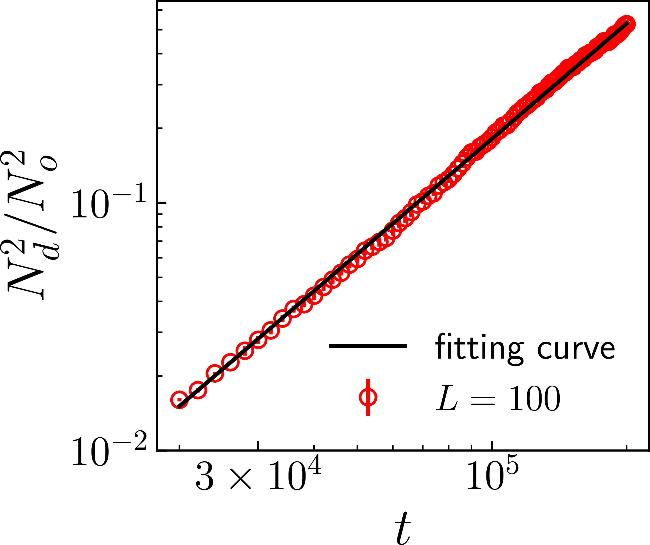
Figure 3. Short-time dynamics of the ratio ${N}_{d}^{2}/{N}_{o}^{2}$ at the critical point Tc = 0.672 for system size L = 100. The dotted curve represents the Monte Carlo results, while the solid line corresponds to the fitted curve with a power function. Log-log coordinates are used. |
With the dynamic critical exponent z determined, the static critical exponent β/ν can be extracted from the scaling behaviors of ${N}_{d}^{2}$ and ${N}_{o}^{2}$ using the scaling relations (10 ) and (13 ) [45]. For the disordered initial state, the inset of figure 4(a) shows ${N}_{d}^{2}$ as a function of the system size L at a fixed time t = 104. A power-law fit yields ${N}_{d}^{2}\propto {L}^{-3.12}$ with the exponent close to d = 3, thereby verifying ${N}_{d}^{2}\propto {L}^{-d}$, as shown in equation (10 ). Then, in the main plot of figure 4(a), by fitting the slope of the curve of ${N}_{d}^{2}$ versus t for L = 100 in log-log coordinates, we find that (d − 2β/ν)/z = 0.957(2), leading to β/ν = 0.581(5) with z = 1.92(1) and d = 3. Figure 4(b) shows the short-time dynamics of ${N}_{d}^{2}$ for different system sizes. In particular, in the time range t ∈ [2 × 10⁴, 2 × 10⁵], the curves in log-log coordinates for L = 100 and L = 80 are almost parallel, demonstrating that the exponent estimated above is almost independent of size. Additionally, by rescaling ${N}_{d}^{2}$ and t as ${N}_{d}^{2}{L}^{2\beta /\nu z}$ and tL−z, the rescaled curves collapse well, as shown in figure 4(c). This collapse indicates that the short-time dynamics of ${N}_{d}^{2}$ obeys the scaling form given in equation (7 ), and supports the estimated critical exponents β/ν and z.
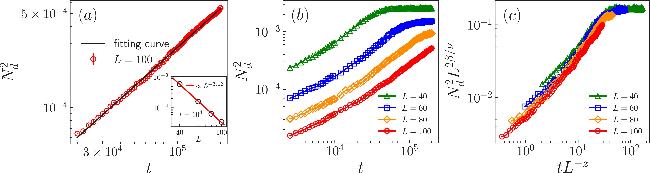
Figure 4. Short-time dynamics of the classical dimer model quenched from a disordered state to the critical point for various system sizes. (a) ${N}_{d}^{2}$ plotted versus time in log-log scale for system size L = 100. The symbols represent the Monte Carlo results, while the solid line corresponds to the fitted result. The inset shows a log-log plot of ${N}_{d}^{2}$ as a function of system size L = 40, 60, 80, 100 at a fixed time t = 104, where the solid line represents a power-law fit yielding ${N}_{d}^{2}\propto {L}^{-3.12}$, consistent with the expected L−d scaling with d = 3. (b) Time dependence of ${N}_{d}^{2}$ for L = 40 to 100. (c) After rescaling ${N}_{d}^{2}$ and t as ${N}_{d}^{2}{L}^{2\beta /\nu z}$ and tL−z, all rescaled curves collapse well. Log-log coordinates are used. |
Similarly, for the ordered initial state, the slope of the curve of ${N}_{o}^{2}$ versus t in log-log coordinates for L = 100 yields −2β/νz = − 0.601(3), leading to β/ν = 0.577(4), as shown in figure 5(a). This value is close to the one obtained from the disordered case. In addition, figure 5(b) shows that the evolution of ${N}_{o}^{2}$ is almost independent of the system size in the short-time stage. By performing the rescaling for ${N}_{o}^{2}$ and t as ${N}_{o}^{2}{L}^{2\beta /\nu z}$ and tL−z, respectively, the curves collapse well, as illustrated in figure 5(c), which not only supports the estimated exponent β/ν and z but also verifies the dynamic scaling form equation (7 ).
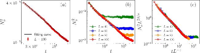
Figure 5. Short-time dynamics of the classical dimer model quenched from an ordered state to the critical point for various system sizes. (a) ${N}_{o}^{2}$ plotted versus time in log-log scale for system size L = 100. (b) Time dependence of ${N}_{o}^{2}$ for L = 40 to 100. (c) After rescaling ${N}_{o}^{2}$ and t as ${N}_{o}^{2}{L}^{2\beta /\nu z}$ and tL−z, all curves collapse well. Log-log coordinates are used. |
Moreover, the values of β/ν obtained via the short-time dynamics from both the ordered and disordered initial states are consistent with previous results. In particular, combining the results η = 0.25(3) and ν = 0.63(4) presented in [34] and the scaling laws, one obtains β = 0.40(7), leading to β/ν = 0.6(1), which is consistent with our present results within the error bar.
Besides these usual long-time critical exponents, the short-time critical dynamics has an additional critical initial slip exponent θ, which can be extracted from the scaling behavior of the time-correlation function, as shown in equation (12 ). Figure 6(a) shows the evolution of Q for L = 80 in the time range t ∈ [2.2 × 10², 2.2 × 10³]. Power fit of the data yields the exponent θ = − 1.052(5). In addition, by rescaling Q and t as QL−θz and tL−z with the exponents θ and z obtained, the rescaled curves collapse well after a transient time, as shown in figure 6(b), which not only confirms the value of θ but also verifies the scaling form equation (11 ).
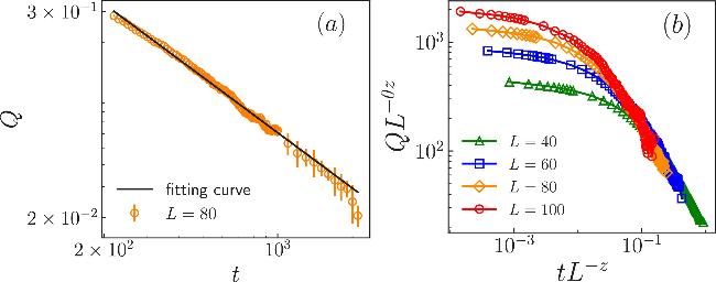


Figure 6. The time correlation of the total order parameter Q starting from a disordered state at the critical point. (a) Time dependence of Q for system size L = 80. Since the statistical fluctuations for L = 100 are too large to allow for a reliable fit, we therefore use L = 80 in our analysis. (b) After rescaling Q and t as QL−θz and tL−z, all curves collapse well. Log-log coordinates are used. |
A striking observation is that θ takes on a negative value here, which stands in contrast to the usual cases in the LGW transitions. When initial states are random and possess a small residual initial order parameter m0, the order parameters' evolution is regulated by two competing effects: critical fluctuations induce its decay, while domain formation arises because the residual m0 tends to orient the neighboring order parameter toward the ordered state. In usual cases, the positive θ indicates that the latter element dominates and the order parameter, say m, will increase as m ∼ m0tθ [40]. The reason is that in the initial stage, there are no long-range correlations, so the system can be described by mean-field theory. In a typical LGW phase transition, critical fluctuations cause the actual critical temperature to be lower than its mean-field counterpart. Thus, in the short-time stage, the system behaves as if it were in an ordered phase, making domain formation the dominant factor in early evolution.
In contrast, in the present case, the critical point has emergent SO(5) symmetry, which describes the rotation symmetry between five components of critical modes in both sides of the critical point. These modes include not only the three components of the order parameter—whose fluctuations tend to drive the critical point below its mean-field value—but also the two additional components that emerge in the disordered phase and drive the critical point in the opposite direction. The emergent SO(5) demonstrates that the strength of fluctuations on both sides of the critical point is essentially the same. Therefore, critical fluctuations cannot cause a qualitative change in the real critical point compared to the mean-field critical point. Accordingly, the domain formation cannot govern the short-time dynamics, resulting in a negative θ.
The behavior that the critical point does not shift to values smaller than its mean-field value due to such additional degrees of freedom is analogous to that observed at Dirac criticality, wherein the order parameter fluctuations drive the critical point below its mean-field value, but the fermion fluctuations play opposite roles. It was shown that when the fermion fluctuations dominate, a negative θ also appears [57, 60].
Another possible reason for the reduction of θ is the presence of the Gauss law in the dimer model [17–21]. This constraint is equivalent to a local conservation law for the gauge charge, which can fundamentally alter the dynamics of the system. Such a constraint can hinder the local rearrangements required for the growth of ordered domains in the early-time regime. Consequently, the amplification of a small initial order parameter is suppressed. As reported in previous literature [73], which shows that a globally conserved order parameter suppresses critical initial slip, we thus speculate that local constraints may do the same, resulting in a negative θ.
It should be noted that these two factors are independent, and we cannot rule out either. We expect to further verify our conclusions in similar models without emergent symmetries or local constraints in future work.
5. Summary
In conclusion, we have systematically investigated the short-time critical dynamics of the 3D classical cubic dimer model using Monte Carlo simulations. By employing the short-time scaling method, we have obtained a comprehensive set of critical parameters without requiring full equilibration of the system, thereby offering an efficient alternative to conventional equilibrium studies.
We have accurately determined the critical temperature Tc = 0.672(1), which is in excellent agreement with values previously reported in the literature. The static critical exponent ratio β/ν = 0.581(5), extracted from the short-time power-law scaling of the order parameter, is also consistent with equilibrium results, validating the reliability of the dynamical approach. Furthermore, we have computed the dynamic critical exponent z = 1.92(1), which governs the temporal scaling of correlation lengths and is in accord with theoretical expectations for a diffusive conserved order parameter [74].
The most striking outcome of our work is the determination of the critical initial slip exponent θ = − 1.052(5). This negative value stands in sharp contrast to the positive θ commonly found in conventional phase transitions described by the LGW paradigm. We attribute this anomalous behavior to two fundamental features of the dimer model at criticality: (i) the emergent SO(5) symmetry, which enhances fluctuation channels and suppresses early ordering, and (ii) the local U(1) gauge constraint (Gauss law), which imposes a conserved diffusive dynamics and slows down the early growth of the order parameter. The negative θ indicates that the order parameter undergoes an initial decay or remains suppressed before the onset of growth, a distinctive signature of the unconventional criticality present in this system.
Our study not only provides the first complete characterization of nonequilibrium short-time criticality in the 3D classical dimer model but also establishes a direct link between its exotic equilibrium universality class and distinctive dynamical scaling laws. The successful application of short-time dynamics in this context demonstrates its power as a robust numerical tool for probing critical phenomena in systems with complex constraints and emergent symmetries. In particular, these results may offer useful hints for understanding nonequilibrium dynamics near deconfined quantum critical points in related quantum systems, where emergent symmetries and gauge constraints also play an important role. For example, studying quantum matter using quantum computers has recently represented an emerging direction, wherein ground-state search relies on imaginary-time evolution. It was shown that imaginary-time evolution near the critical point obeys scaling similar to that of classical relaxation dynamics [55, 61]. The work thus not only motivates us to further investigate the imaginary-time relaxation dynamics at the deconfined critical point, but also bears important implications for the experimental realization of novel quantum devices hosting similar deconfined critical points.