

1. Introduction
Majorana bound states (MBSs), as non-Abelian anyons governed by non-Abelian statistics, have become a core building block for topological quantum computing in recent years [1–4]. Quantum dot (QD) systems coupled with superconductors serve as a highly flexible platform for engineering and manipulating MBS. Experimental advances—including observations of zero-bias conductance peaks in QD-superconductor hybrids—have yielded indirect but compelling evidence for MBS existence [5–7]. It is well established that MBS detection can be achieved by measuring transport current through QDs. This lays a solid foundation for developing complex hybrid Majorana-QD systems [8, 9]. Theoretically, multi-band models and strong correlation frameworks have refined descriptions of MBS localization at QD-superconductor interfaces, showing that gate voltage, magnetic field, and superconducting pairing potential can be tuned to control MBS binding and coherence [10–13]. For instance, QDs hybridized with topological quantum wires enable investigations into the intrinsic physical properties. Further refining theoretical models and clarifying the underlying physics of these systems is therefore essential, given that strong repulsive Coulomb interactions in QDs coupled to ferromagnetic (FM) leads trigger the Kondo effect at low temperatures [14–16]. When integrated with MBS, the Majorana–Kondo (M–K) effect generates unique quantum coherence and transport behaviors. Recent theoretical predictions indicate that the M–K interaction can modulate MBS coherence, induce topological phase transitions, and produce novel spin-dependent transport signatures [17–20]. However, the mechanism sustaining Kondo screening in the presence of Majorana fermions remains incompletely understood. Given that the interplay between QD Kondo physics and Majorana physics dominates topological superconductor behaviors [21–23], it is essential to investigate the Kondo resonance within QDs can be suppressed by an exchange field induced by lead spin polarization.
Meanwhile, coupling between QDs and phonons is another key factor governing charge transport, energy relaxation, and coherence dynamics in low-dimensional systems [24–26]. In conventional semiconductor QDs, electron–phonon (e-ph) interactions induce phenomena like phonon-assisted tunneling, spectral linewidth broadening, and electronic state decoherence. Phonon modes exert distinct effects depending on QD size, material properties, and temperature [27, 28]. Acoustic phonons dominate energy relaxation in small QDs via deformation potential coupling, while optical phonons contribute significantly to inelastic scattering in polar semiconductor QDs. Recent progress in nanomechanics has enabled tuning e-ph interaction strength through strain engineering or piezoelectric effects, opening new pathways to modulate QD electronic properties [29–31]. Additionally, spin-polarized transport in MBS-QD systems is vital for quantum information science, enabling spin-charge interconversion essential to spintronic and spin-based quantum computing [32–36]. Yet, integrating e-ph interactions with the M–K interplay in MBS-QD systems has not been extensively studied. Can the M–K interplay mitigate phonon-induced MBS dephasing, or the reverse occur? These questions create a critical gap between fundamental MBS physics and practical device development.
Against this backdrop, this study develops a unified theoretical framework for MBS-QD hybrid systems, explicitly incorporating the M–K interaction, e-ph interaction, and spin polarization—under the realistic condition of infinite Coulomb repulsion (which suppresses QD double occupancy, a key prerequisite for the M–K effect). We systematically investigate how these three factors synergistically regulate spin-dependent transport properties, focusing on the M–K interpaly modulation of e-ph-induced transport behaviors under the combined constraints of strong Coulomb correlation. Our findings aim to provide specific theoretical guidance for experimental MBS detection via Kondo-enhanced transport.
2. Model and method
In this paper, we consider the e-ph interaction process in a coupled Majorana-QD system with two FM leads (see figure 1). The e-ph interaction takes place in the QD region with an optical phonon mode of frequency ω0. Then the studied system can be described by the following Hamiltonian1 ) describes the phonon mode
$\begin{eqnarray}H={H}_{{\rm{L}}{\rm{e}}{\rm{a}}{\rm{d}}}+{H}_{{\rm{p}}{\rm{h}}}+{H}_{{\rm{D}}}+{H}_{{\rm{M}}{\rm{B}}}+{H}_{{\rm{T}}}.\end{eqnarray}$
$\begin{eqnarray}{H}_{{\rm{L}}{\rm{e}}{\rm{a}}{\rm{d}}}=\displaystyle \displaystyle \sum _{{k}_{\alpha },\sigma }{\varepsilon }_{{k}_{\alpha }\sigma }{c}_{{k}_{\alpha }\sigma }^{+}{c}_{{k}_{\alpha }\sigma }.\end{eqnarray}$
${c}_{{k}_{\alpha }\sigma }^{+}({c}_{{k}_{\alpha }\sigma })$ is the creation (annihilation) operator for an electron with spin σ, momentum k and energy ${\varepsilon }_{{k}_{\alpha }\sigma }$ in the lead [α = left (L) or right (R)]. The second term in equation ( $\begin{eqnarray}{H}_{{\rm{p}}{\rm{h}}}=\hslash {\omega }_{0}\left({b}^{+}b\right)+\lambda \displaystyle {\sum }_{\sigma }\left({b}^{+}+b\right){d}_{\sigma }^{+}{d}_{\sigma },\end{eqnarray}$
where ${b}^{+}(b)$ is the creation (annihilation) operator of the phonon mode. Physically, ${\omega }_{0}$ corresponds to the frequency of a long-wavelength optical phonon mode. λ is the e-ph interaction strength between the QD electron and the phonon mode. This parameter range allows us to systematically explore the competition between phonon-assisted resonant tunneling and phonon-induced decoherence. $\begin{eqnarray}{H}_{{\rm{D}}}=\displaystyle \displaystyle \sum _{\sigma }{\varepsilon }_{d\sigma }{d}_{\sigma }^{+}{d}_{\sigma }+U{{n}}_{\uparrow }{{n}}_{\downarrow },\end{eqnarray}$
where ${d}_{\sigma }^{+}({d}_{\sigma })$ is the creation (annihilation) operator for the QD with energy ${\varepsilon }_{d\sigma }$. U is chosen to be sufficiently large to suppresses double occupancy of the QD (i.e. only one electron can occupy the QD at a time). Such a choice simplifies the theoretical treatment while retaining the essential correlation effects of QD electrons. Under ideal conditions (no impurity scattering, low temperature), the spin polarization of FM electrodes and the non-Abelian properties of Majorana fermions jointly suppress charge transport, making the lead current approach zero. Furthermore, the phonon-assisted tunneling of quasiparticles is induced. The interface coupling between the QD and the FM electrode may generate a weak current. In the present model, we assume that the superconducting wire remains in thermodynamic equilibrium with a fixed chemical potential. Under this approximation, the current distribution inside the Majorana wire does not affect the transport calculations in the QD region. $\begin{eqnarray}{H}_{{\rm{M}}{\rm{B}}}={\rm{i}}{\varepsilon }_{{\rm{M}}}{\gamma }_{1}{\gamma }_{2},\end{eqnarray}$
is the Majorana wire Hamiltonian. γ1 and γ2 are the Majorana operator at the two ends of the superconducting nanowire. ${\varepsilon }_{{\rm{M}}}$ is the overlap energy corresponding to ${\varepsilon }_{{\rm{M}}}\propto \exp [-L/\xi ]$, with L the topological superconducting nanowire length and ξ is the superconducting coherence length.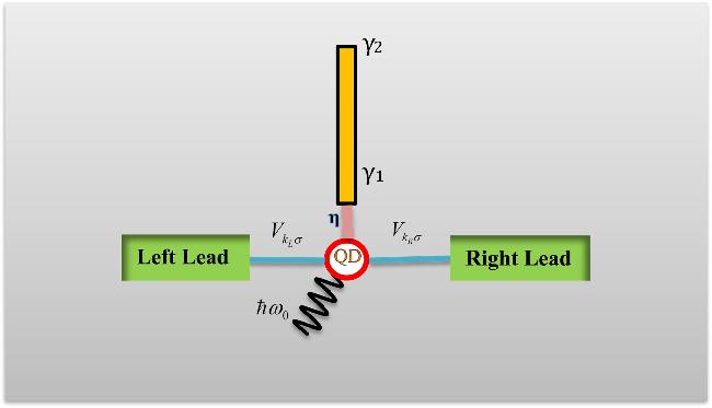
Figure 1. Schematic representation of the phonon-assisted Majorana-QD system, which is coupled to MBS located at the ends of a one dimensional topological superconductor nanowire with the coupling strength η. The electron–phonon interaction takes place in QD region with a single long-wave optical phonon mode of frequency ${\omega }_{0}$. The QD is also connected with the ferromagnetic (FM) leads through the tunnel matrix elements ${V}_{{k}_{\alpha }\sigma }(\alpha =L,R)$. |
The last term in equation (1 ) describes the MBS-QD couplings and the QD-leads couplings.
$\begin{eqnarray}{H}_{{\rm{T}}}={\sum }_{\sigma }\left(\eta {d}_{\sigma }-{\eta }^{\ast }{d}_{\sigma }^{+}\right){\gamma }_{1}+\displaystyle \sum _{{k}_{\alpha }\sigma }\left({V}_{{k}_{\alpha }\sigma }{c}_{k\alpha \sigma }^{+}{d}_{\sigma }+{\rm{h}}.{\rm{c}}.\right),\end{eqnarray}$
where $\eta $ represent the MBS-QD coupling strength. ${V}_{{{k}}_{\alpha }\sigma }$ denotes the tunnel elements between the QD and the lead α. It also leads to an energy independent function ${{\rm{\Gamma }}}_{\sigma }^{\alpha }=\pi \displaystyle \displaystyle \sum _{{{k}}_{\alpha }\sigma }{\left|{V}_{{{k}}_{\alpha }\sigma }\right|}^{2}\delta \left(\varepsilon -{\varepsilon }_{{k}\alpha \sigma }\right)$ in the spin dependent calculation. ‘h.c.' stands for Hermitian conjugate to ensure the Hamiltonian is Hermitian. We then define the spin-up and spin-down dependent coupling strength for the electrode as ${{\rm{\Gamma }}}_{\uparrow \downarrow }^{\alpha }=\left(1\pm p\right){{\rm{\Gamma }}}_{0}$($\uparrow \downarrow $ represents the spin-up and spin down coupling), where p represents the strength of spin polarization. ${{\rm{\Gamma }}}_{0}$ is the value at p = 0 and set to be the unit in our numerical results.We use the equivalent regular Majorana representation to represent the Majorana fermion. Namely, ${\gamma }_{1}$ and ${\gamma }_{2}$ can be replaced by ${\gamma }_{1}=\left({f}_{{\rm{M}}}+{f}_{{\rm{M}}}^{+}\right)/\sqrt{2}\,$ and ${\gamma }_{2}=-{\rm{i}}({f}_{{\rm{M}}}-{f}_{{\rm{M}}}^{+})/\sqrt{2}$, which transforms HMB and HT as
$\begin{eqnarray}{H}_{{\rm{M}}{\rm{B}}}={\varepsilon }_{{\rm{M}}}\left({f}_{{\rm{M}}}^{+}{f}_{{\rm{M}}}-\displaystyle \frac{1}{2}\right),\end{eqnarray}$
$\begin{eqnarray}\begin{array}{rcl}{H}_{{\rm{T}}} & = & \displaystyle \frac{1}{\sqrt{2}}{\sum }_{\sigma }\left(\eta {d}_{\sigma }-{\eta }^{\ast }{d}_{\sigma }^{+}\right)\left({f}_{{\rm{M}}}+{f}_{{\rm{M}}}^{+}\right)\\ & & +\,\displaystyle \sum _{{k}_{\alpha }\sigma }\left({V}_{{k}_{\alpha }\sigma }{c}_{k\alpha \sigma }^{+}{d}_{\sigma }+{\rm{h}}.{\rm{c}}.\right).\end{array}\end{eqnarray}$
By mapping the e-ph interaction effects onto renormalized parameters, the transformation reduces the problem to a more tractable electronic Hamiltonian, enabling systematic derivation of key transport quantities while retaining the essential physics of e-ph interaction. Thus, we apply a canonical transformation $\tilde{H}={{\rm{e}}}^{S}H{{\rm{e}}}^{-S}$ with $S=\displaystyle \frac{\gamma }{{\omega }_{0}}{d}_{\sigma }^{+}{d}_{\sigma }\left({b}^{+}-b\right)$, which has been used to manage the effects of e-ph interaction on the localized states [37, 38]. Specifically, by unitarily transforming the original Hamiltonian, the transformation eliminates the explicit cross term between electronic operators (${d}_{\sigma }^{+},{d}_{\sigma }$) and phonon operators (${b}^{+},b$) that characterizes direct e-ph interaction. Instead, it incorporates the influence of e-ph interaction into two key aspects of the effective Hamiltonian: the QD energy level (which acquires a phonon-induced shift) and the coupling strengths between the QD and external subsystems (i.e. the MBS-QD coupling and QD-FM lead tunneling elements, both renormalized by a factor related to phonon occupation). This crucial simplification avoids the need to directly solve the many-body problem involving coupled electron and phonon degrees of freedom. The transformed Hamiltonian becomes $\tilde{H}={\tilde{H}}_{{\rm{e}}}+{H}_{{\rm{p}}{\rm{h}}}$, while the phonon part remains unchanged. The electron term can be written as follows,
$\begin{eqnarray}{\tilde{H}}_{{\rm{e}}}={H}_{{\rm{l}}{\rm{e}}{\rm{a}}{\rm{d}}}+{H}_{{\rm{M}}{\rm{B}}}+{\tilde{H}}_{{\rm{D}}}+{\tilde{H}}_{{\rm{T}}},\end{eqnarray}$
where ${\tilde{H}}_{{\rm{D}}}={\tilde{\varepsilon }}_{d\sigma }{d}_{\sigma }^{+}{d}_{\sigma }+\tilde{U}{n}_{\uparrow }{n}_{\downarrow }$ with ${\tilde{\varepsilon }}_{d\sigma }={\varepsilon }_{d\sigma }-g{\omega }_{0},$ and $\tilde{U}=U-2g{\omega }_{0},g=\displaystyle \frac{{\lambda }^{2}}{{\omega }_{0}^{2}}$. $\begin{eqnarray}{\tilde{H}}_{{\rm{T}}}=\displaystyle \frac{1}{\sqrt{2}}\left(\tilde{\eta }{d}_{\sigma }-{\tilde{\eta }}^{\ast }{d}_{\sigma }^{+}\right)\left({f}_{{\rm{M}}}+{f}_{{\rm{M}}}^{+}\right)+\displaystyle \sum _{{k}_{\alpha }\sigma }\left({\tilde{V}}_{{k}_{\alpha }\sigma }{c}_{k\alpha \sigma }^{+}{d}_{\sigma }+{\rm{h}}.{\rm{c}}.\right).\end{eqnarray}$
In cases of canonical transformation, the QD-lead and MBS-QD coupling elements will be renormalized by introducing a corresponding factor X, which arises from the canonical transformation of the particle operator ${{\rm{e}}}^{-S}d{{\rm{e}}}^{S}=\tilde{d}X$. Namely ${\tilde{V}}_{{k}_{\alpha }\sigma }$ and $\tilde{\eta }\left({\tilde{\eta }}^{\ast }\right)$ will be replaced as ${\tilde{V}}_{{k}_{\alpha }\sigma }={V}_{{k}_{\alpha }\sigma }X$ and $\tilde{\eta }\left({\tilde{\eta }}^{\ast }\right)=\eta \left({\eta }^{\ast }\right)X$ with $X=\exp \left[-\tfrac{\gamma }{{\omega }_{0}}\left({b}^{+}-b\right)\right]$. This means that the interaction between the QD electrons and phonon modes leads to the shift of QD levels and the MBS-QD (lead) couplings. Here, the band narrowing induced by the e-ph interaction will be avoided for unnecessary complications. One reasonable method is to replace the operator X by its expectation value $\left\langle X\right\rangle ={{\rm{e}}}^{-g({N}_{{\rm{p}}{\rm{h}}}+0.5)}$ since $\left\langle X\right\rangle $ only results in a trivial quantitative shift of the tunneling process. Nph is the phonon population expressed as ${N}_{{\rm{p}}{\rm{h}}}={\left({{\rm{e}}}^{{\omega }_{0}/{k}_{{\rm{B}}}T}-1\right)}^{-1}$. Then the QD electron Green's function can be decoupled as
$\begin{eqnarray}\begin{array}{lll}{G}_{d\sigma }^{r}\left(t\right) & = & -{\rm{i}}\theta \left(t\right)\left\langle \left\{{d}_{\sigma }\left(t\right),{d}_{\sigma }^{t}\left(0\right)\right\}\right\rangle \\ & = & -{\rm{i}}\theta \left(t\right)\left\langle \left\{{{\rm{e}}}^{{\rm{i}}{\tilde{H}}_{{\rm{e}}}t}{d}_{\sigma }\left(t\right){{\rm{e}}}^{-{\rm{i}}{\tilde{H}}_{{\rm{e}}}t},{d}_{\sigma }^{t}\left(0\right)\right\}\right\rangle \\ & = & -{\rm{i}}\theta \left(t\right)\left(\left\langle \left\{{\tilde{d}}_{\sigma }\left(t\right),{\tilde{d}}_{\sigma }^{t}\left(0\right)\right\}\right\rangle {\left\langle \left\{X\left(t\right){X}^{+}\left(0\right)\right\}\right\rangle }_{{\rm{p}}{\rm{h}}}\right.\\ & & \left.+\,\left\langle \left\{{\tilde{d}}_{\sigma }^{t}\left(0\right){\tilde{d}}_{\sigma }\left(t\right),\right\}\right\rangle {\left\langle \left\{{X}^{+}\left(0\right)X\left(t\right)\right\}\right\rangle }_{{\rm{p}}{\rm{h}}}\right),\end{array}\end{eqnarray}$
where ${\left\langle X\left(t\right){X}^{+}\left(0\right)\right\rangle }_{{\rm{p}}{\rm{h}}}={{\rm{e}}}^{-\theta \left(t\right)}$, ${\left\langle {X}^{+}\left(0\right)X\left(t\right)\right\rangle }_{{\rm{p}}{\rm{h}}}={{\rm{e}}}^{\theta \left(-t\right)}$ represents the renormalized e-ph interaction induced factor as phonon parts and $\theta \left(t\right)=g\left[{N}_{{\rm{p}}{\rm{h}}}\left(1-{{\rm{e}}}^{{\rm{i}}{\omega }_{0}t}\right)\right.$ + $\left.\left({N}_{{\rm{p}}{\rm{h}}}+1\right)\left(1-{{\rm{e}}}^{-{\rm{i}}{\omega }_{0}t}\right)\right]$.The Fourier transform of the retarded Green's function ${G}_{d\sigma }^{r}(t)$ is given by
$\begin{eqnarray}\begin{array}{lll}{G}_{d\sigma }^{r}\left(\varepsilon \right) & = & \displaystyle \sum _{n=-\infty }^{\infty }{L}_{n}\left[\left(1-\left\langle {n}_{d\sigma }\right\rangle {\tilde{G}}_{d\sigma }^{r}\left(\varepsilon -n{\omega }_{0}\right)\right.\right.\\ & & \left.\left.+\,\left\langle {n}_{d\sigma }\right\rangle {\tilde{G}}_{d\sigma }^{r}\left(\varepsilon +n{\omega }_{0}\right)\right)\right],\end{array}\end{eqnarray}$
where Ln represents the coefficients depending on temperature and the strength of e-ph interaction. At finite temperature, ${L}_{n}=\exp \left[-g\left(2{N}_{{\rm{p}}{\rm{h}}}+1\right)\right]$ × $\exp \left[n{\omega }_{0}/\left(2T\right)\right]\times {J}_{n}\left(2g\sqrt{{N}_{{\rm{p}}{\rm{h}}}\left({N}_{{\rm{p}}{\rm{h}}}+1\right)}\right)$, where ${J}_{n}\left(z\right)$ is the modified complex nth Bessel function with the index n indicating the number of phonons involved. Additionally, ${n}_{d\sigma }$ the average occupation number of the QD—is determined self-consistently via the Fermi distribution function $f\left(\varepsilon \right)=\displaystyle \frac{1}{{{\rm{e}}}^{\left(\varepsilon -{E}_{{\rm{F}}}\right)/T}+1}$, where ${E}_{{\rm{F}}}$ is the Fermi energy (set to 0 in our calculations) and T is the temperature(set to 0.001 in our calculations). We use the equation of motion (EOM) procedure [39–41] to obtain the retarded Green's function $\left({\tilde{G}}_{d\sigma }^{r}\left(\varepsilon \right)=\ll {d}_{\sigma },{d}_{\sigma }^{+}\gg \right)$ of the QD in energy space, which can be written as follows: (see the appendix for explicit derivation process): $\begin{eqnarray}\begin{array}{c}\ll {d}_{\sigma s},{d}_{\sigma }^{+}\gg \\ =\,\displaystyle \frac{1-\left\langle {n}_{d\bar{\sigma }}\right\rangle }{\left[\varepsilon -{\tilde{\varepsilon }}_{d\sigma }-\displaystyle {\sum }_{0}^{r}\left(\varepsilon \right)-\displaystyle {\sum }_{1\sigma }^{r}\left(\varepsilon \right)-{\rm{\Lambda }}\left(\varepsilon \right)-{\tilde{\eta }}^{2}\kappa +{{\rm{\Omega }}}_{1}\left(\varepsilon \right)-{\rm{\Xi }}\left(\varepsilon \right)\right]}\\ \times \,\left(U\to \infty \right),\end{array}\end{eqnarray}$
where $\displaystyle {\sum }_{1\left(2\right)\sigma }^{r}\left(\varepsilon \right)$ and ${\rm{\Xi }}\left(\varepsilon \right)$ are defined as $\displaystyle {\sum }_{1\left(2\right)\sigma }^{r}\left(\varepsilon \right)\,=\displaystyle \displaystyle \sum _{k\alpha \sigma }\displaystyle \frac{{\left|{\tilde{V}}_{k\alpha \sigma }\right|}^{2}f\left({\varepsilon }_{k\alpha \bar{\sigma }}\right)}{\left(\varepsilon \mp {\tilde{\varepsilon }}_{d\sigma }\pm {\tilde{\varepsilon }}_{d\bar{\sigma }}-{\varepsilon }_{k\alpha \bar{\sigma }}\right)}$ $\begin{eqnarray*}{\rm{\Xi }}\left(\varepsilon \right)=\displaystyle \frac{\left({\tilde{\eta }}^{2}\kappa -{{\rm{\Omega }}}_{1}\left(\varepsilon \right)\right)\left({\tilde{\eta }}^{2}\kappa -{{\rm{\Omega }}}_{2}\left(\varepsilon \right)\right)}{\varepsilon +{\tilde{\varepsilon }}_{d\sigma }-\displaystyle {\sum }_{0}^{r}\left(\varepsilon \right)-\displaystyle {\sum }_{2\sigma }^{r}\left(\varepsilon \right)-{\rm{\Lambda }}\left(\varepsilon \right)-{\tilde{\eta }}^{2}\kappa +{{\rm{\Omega }}}_{2}\left(\varepsilon \right)}.\end{eqnarray*}$
The explicit relation for the occupation number can be described by: $\begin{eqnarray*}\lt {n}_{d\sigma }\gt =-\displaystyle \frac{1}{\pi }\displaystyle \int \displaystyle \frac{{{\rm{\Gamma }}}_{\sigma }^{L}{f}_{L}(\varepsilon )+{{\rm{\Gamma }}}_{\sigma }^{R}{f}_{R}(\varepsilon )}{{{\rm{\Gamma }}}_{\sigma }^{L}+{{\rm{\Gamma }}}_{\sigma }^{R}}\rm{Im}\left[{\tilde{G}}_{d\sigma }^{r}\left(\varepsilon \right)\right]{\rm{d}}\varepsilon ,\end{eqnarray*}$
where the Fermi distribution function weights the contribution of each energy level to the average occupation number.3. Results and discussions
This section focuses on unraveling the synergistic regulatory mechanisms of the M–K interaction, e-ph interaction, and spin polarization strength in shaping conductance and density of states (DOS) behaviors.
3.1. Linear conductance regulation by ϵM without e-ph interaction
First, we investigated the linear conductance $\left({G}_{\sigma }=\displaystyle \displaystyle {\sum }_{\sigma }\tfrac{{{\rm{\Gamma }}}_{\sigma }^{L}\cdot {{\rm{\Gamma }}}_{\sigma }^{R}}{{{\rm{\Gamma }}}_{\sigma }^{L}+{{\rm{\Gamma }}}_{\sigma }^{R}}{\left.\rm{Im}\left[{G}_{d\sigma }^{r}\left(\varepsilon \right)\right]\right|}_{\varepsilon =0}\right)$ as a function of the Majorana overlap energy for different ${\varepsilon }_{d}$ without e-ph interaction in figure 2. When ${\epsilon }_{{\rm{M}}}=0$ (corresponding to an infinite long Majorana topological superconducting wire), the two Majorana fermions form a Majorana zero mode with particle-hole symmetry. The QD acts as a resonant cavity, the self-energy term diverges as $\varepsilon \to 0$. Consequently, the QD couples to the Majorana zero mode to form a fully localized bound state. Because the QD is decoupled from the external leads, the transmission vanishes and the conductance becomes zero. For finite-length Majorana-coupled leads (${\epsilon }_{{\rm{M}}}\ne 0$), the Majorana bound-state degeneracy is lifted, the conductance recovers to a finite value that varies with the QD level and the tunneling coupling strengths. The zero conductance phenomenon can serve as an important criterion to distinguish a genuine Majorana zero mode from trivial Andreev bound states. Figures 2(a)–(d) shows that linear conductance G first increases with ${\,\varepsilon }_{{\rm{M}}}$, reaches a peak, then decreases, and finally stabilizes. As ${\,\varepsilon }_{d}$ increases, the conductance peak becomes higher and broader, and its position shifts to the left (from ${\varepsilon }_{{\rm{M}}}\approx 2.0$ to ${\varepsilon }_{{\rm{M}}}\approx 1.0$). Increasing ${\varepsilon }_{{\rm{M}}}$ screens the local spin moments induced by MBS-QD coupling. This also reduces the dephasing of hybrid states. As ${\varepsilon }_{d}$ increases, the M–K interaction increases, further amplifying the resonance effect, leading to a higher tunneling probability and thus a more prominent conductance peak. When ${\varepsilon }_{{\rm{M}}}\,$ is far from the resonance interval, the degree of energy level matching between the QD and MBS decreases, but the M–K interaction still maintains a certain level of resonant channel connectivity, resulting in slower decrease in conductance.
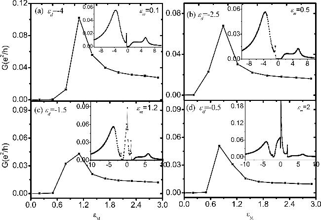
Figure 2. Linear conductance as a function of ${\varepsilon }_{{\rm{M}}}$ under different ${\varepsilon }_{d}$ without e-ph interaction. The parameters are chosen as $p=0.0;\,\eta =3{;}\,T=0.001$. Each subpanel shows the DOS under different majorana energy level ${\varepsilon }_{{\rm{M}}}$ for the corresponding electron–phonon coupling strength $\lambda =0.0;\,{\varepsilon }_{d}=-4$. |
We added subgraphs to each figure in figure 2 to discuss the DOS $\left({\rm{DOS}}=-\displaystyle \frac{1}{\pi }\rm{Im}\left[{G}_{d\sigma }^{r}\right]\right)$ after introducing different ${\varepsilon }_{{\rm{M}}}$. It can be observed that with the increase of Majorana overlap energy, an obvious resonant peak is formed near the Fermi level. Compared with the ‘no-Majorana' case, the resonance is strongly enhanced because the QD level now lies inside the Kondo region. Hence the side peaks are interpreted as the ordinary Kondo side-bands that are pushed away from the Fermi level by the coupling to the Majorana mode, whereas the peak at $\varepsilon =0$ is the induced zero-mode resonance characteristic.
3.2. Modulation of e-ph interaction on conductance and DOS
To further demonstrate the correlation effect between the MBS and QD, we introduced the linear conductance under the condition of e-ph interaction (different e-ph interaction λ) in figure 3. For different ${\varepsilon }_{{\rm{M}}}$ (0.1, 0.5, 1.0, 2.0), the conductance first rises to a peak then decreases to a stable value as λ increases. Compared to systems without e-ph interaction (figure 2), the peak position shifts to the right from λ = 0.3 to λ = 0.6, and the decay rate of conductance in the strong e-ph regime is significantly reduced. The peak of G increases with ${\varepsilon }_{{\rm{M}}}$ (e.g. G = 0.008 for ${\varepsilon }_{{\rm{M}}}$ = 0.1, G = 0.07 for ϵM = 2.0), which is attributed to the combined effects of enhanced MBS-QD interaction. Larger ${\varepsilon }_{{\rm{M}}}$ increases the overlap between MBS and QD states, which in turn cooperates with phonon-assisted tunneling to enhance conductance. In the weak e-ph regime (λ < 0.3). The e-ph interaction adjusts the energy level matching between MBS and QD, leading to an increase of conductance with λ. Moderate λ (0.3–0.7) optimizes this synergy, yielding the maximum conductance. When λ exceeds a certain value, phonon-induced decoherence becomes dominant. A larger ${\varepsilon }_{{\rm{M}}}$ requires a stronger λ to compensate for energy level mismatch, explaining the peak shift and higher peak conductance. Additionally, a small ${\varepsilon }_{{\rm{M}}}$ leads to a narrow resonance window between QD and MBS. The M–K interaction partially suppresses the deleterious effects of e-ph interaction on the conductance resonance, resulting in a more sensitive dependence on λ.
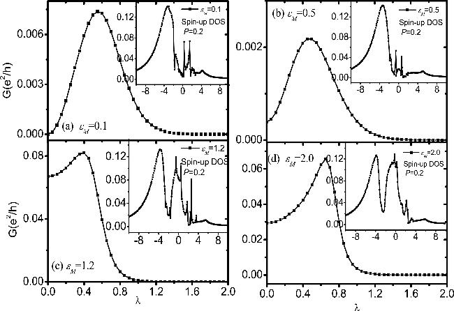
Figure 3. Linear conductance as a function of electron–phonon interaction strength $\lambda $ under different ${\varepsilon }_{{\rm{M}}}$. The parameters are chosen as $p=0.0;\,\eta =0.5;\,{\varepsilon }_{d}=-3.5{;}\,T=0.001$. Each subpanel shows the DOS under different majorana energy level ${\varepsilon }_{{\rm{M}}}\,$ for the corresponding electron–phonon coupling strength $\lambda =1.0;\,\eta =2.5;\,{\varepsilon }_{d}=-4$. |
We also analyze the evolution of spin-up DOS with different ${\varepsilon }_{{\rm{M}}}$ under the influence of e-ph interaction from each sub-figure in figure 3. In the low-energy region (${\varepsilon \unicode{x0007E}\varepsilon }_{d}$), there is a prominent peak, which originates from the M–K interaction of the QD. The DOS around the zero-energy becomes distinct and intense, reducing the dephasing of hybrid states and enhancing coherence. When $\,{\varepsilon }_{{\rm{M}}}$ further increases (${\varepsilon }_{{\rm{M}}}=1.2\,\mathrm{or}\,2.0$), the DOS evolves from ‘sharp coherent structures' to ‘dispersed multi-peak structures'. The multi-peak DOS aligns with the phonon-assisted tunneling from the e-ph interaction, which enables electrons to transition between different energies via phonon emission/absorption.
3.3. Conductance and DOS dependence on ${\varepsilon }_{{d}\,}$ under the e-ph interaction
We then investigated the variation of conductance with ${\varepsilon }_{d}$ for different e-ph interaction strengths λ (figure 4). Figure 4(a) shows that G decreases with ${\varepsilon }_{d}$ when λ = 0. When the e-ph interaction is introduced [λ = 0.5, figure 4(b)], the conductance exhibits a more pronounced peak. This broadens the phonon-assisted tunneling channels, and the M–K interaction amplifies the resonance gain, resulting a peak in the conductance. For larger λ [figure 4(c)], we found that the linear conductance decreases. However, the conductance shows a monotonic increasing trend as $\,{\varepsilon }_{d}$ increase. When λ is further increased to λ = 1.5 [figure 4(d)], high-order multi-phonon processes govern the tunneling. The M–K mechanism is no longer able to counter the strong decoherence, the conductance drops sharply.
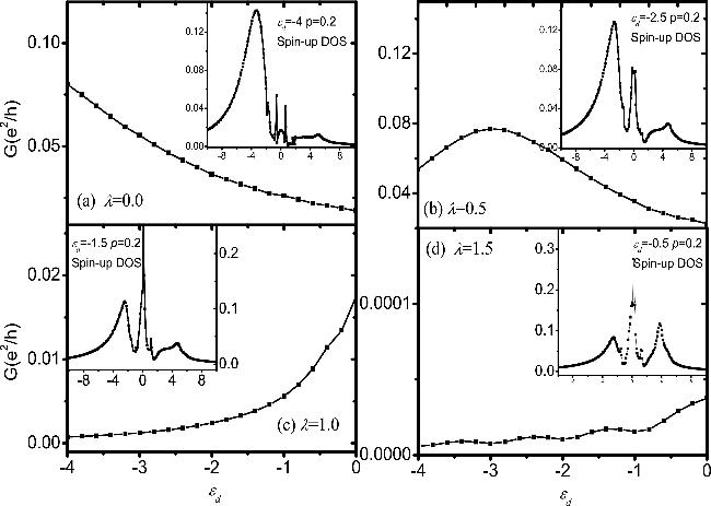
Figure 4. Linear conductance as a function of ${\varepsilon }_{d}$ under different $\,\lambda $. The parameters are chosen as $p=0.0;\,\eta =0.5;\,{\varepsilon }_{{\rm{M}}}=1.2{;}\,T=0.001$. Each subpanel shows the DOS under different majorana energy level ${\varepsilon }_{d}$ for the corresponding electron–phonon coupling strength $\lambda =0.5;\,\eta =2.5;\,{\varepsilon }_{{\rm{M}}}=1.2$. |
We also illustrate how the spin-up DOS shifts as$\,{\varepsilon }_{d}$ changes in the sub-panels of figures 4(a)–(d). In addition to the resonance peak structure in the region where $\varepsilon ={\varepsilon }_{{d}}$ (related to the energy levels of QD), we also found that another peak structure appears near the Fermi energy. This peak structure increases as ${\varepsilon }_{d}$ increases. This reflects the resonant interaction between Majorana fermions and the QD occulting. When ${\varepsilon }_{d}\,$is far from the Fermi energy (${\varepsilon }_{d}=-4$), the low electron occupation of QD leads to a narrow single peak in DOS with weak e-ph-induced broadening. As ${\varepsilon }_{d}$ increases (${\varepsilon }_{d}=-2.5$), the spin-up electron occupation of QD increases (${n}_{d\uparrow }\,\uparrow $), and the probability of electron–phonon scattering increases, leading to moderate peak broadening. When ${\varepsilon }_{d}$ further increases to −1.5, the M–K interaction is significantly enhanced, resulting in a prominent zero-energy resonance peak and a secondary peak in the positive energy region. When ${\varepsilon }_{d}$ is close to the Fermi energy (${\varepsilon }_{d}=-0.5$), the interaction reaches its maximum, and the DOS exhibits a strong zero-energy resonance peak and distinct high-energy phonon side peaks.
3.4. Spin-dependent DOS: amplification of asymmetry by M–K interplay
Finally, we examine the spin-dependent DOS under different spin polarization strengths (p) of FM electrodes taking full account of the M–K interaction (figure 5). When the electrode is non-spin-polarized [p = 0, figure 5(a)], the DOS exhibits a single broad peak, dominated by the M–K-enhanced MBS-QD hybrid state. In the case of weak spin polarization [p = 0.2, figure 5(b)], the peak intensity of spin-up DOS increases, while spin-down DOS decreases [sub-figure in figure 5(b)]. This asymmetry arises from the spin-dependent screening of local moments. Despite the decrease in overall peak intensity, the single broad peak profile is retained because weak spin polarization marginally perturbs the M–K-induced resonance. When spin polarization increases to p = 0.6 [figure 5(c)], the spin-up DOS peak becomes more intense and sharper, while the spin-down DOS peak is suppressed and broadened. The M–K interaction strengthens the spin selectivity of MBS-QD coupling—spin-up electrons, which have the same magnetization direction as the FM leads, experience enhanced M–K screening, reducing dephasing and promoting resonant tunneling, while spin-down electrons face a higher tunneling barrier, leading to suppressed DOS. As the spin polarization strength increases further [p = 0.8, figure 5(d)], in addition to the resonance peak near $\varepsilon ={\varepsilon }_{{d}}$, numerous satellite peaks also emerge near the Fermi energy. As shown in figures 5(c) and (d), spin polarization splits the DOS near zero energy into distinct satellite peaks. For spin-polarized lead (p ≠ 0), the electron-lead interactions can induce an asymmetric occupation number (${n}_{d\uparrow }\ne {n}_{d\downarrow }$), which gives rise to the exchange interaction in the FM lead [42]. When MBSs are introduced and coupled to the QD, they rescale the effective energy level positions of the QD, resulting in a strong spin asymmetry in its response to the FM exchange field. If the hybridization between the MBS and the spin-up state of the QD is strong, the energy shift induced by this hybridization cancels part of the splitting effect of the FM exchange field on the spin-up state, rendering the spin-up channel Kondo-active. Specifically, the spin-dependent hybridization causes the spin occupancy number to decrease, thus, the DOS inevitably splits with the increase of p, leading to multiple-peak splitting. Notably, the amplitude of spin-up DOS is consistently higher than that of spin-down DOS in the inset of figure 5(d), which is consistent with the ‘spin filtering' effect of FM polarization—the M–K interaction further enhances this filtering efficiency by enhancing the transport efficiency of spin-up electrons. In contrast, the weaker hybridization with the spin-down state suppresses the Kondo resonance of the spin-down channel, confining it to a Kondo-inactive state. As spin polarization increases, the modification of the DOS near zero energy significantly shapes the spin-asymmetric DOS structure. This finding offers a theoretical basis for developing high-efficiency MBS-based spin filters.
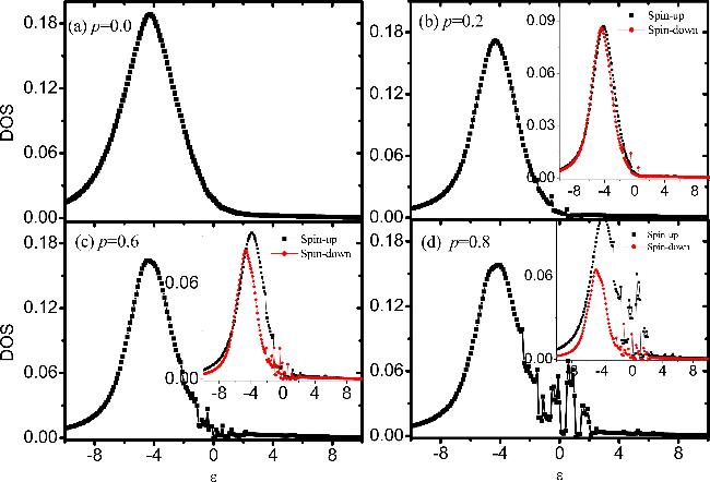


Figure 5. The DOS under different p. The parameters are chosen as $\lambda =1.0;\,\eta =2.5;\,{\varepsilon }_{{\rm{M}}}=0.1;\,{\varepsilon }_{d}=-4{;}\,T=0.001.\,$ Each subpanel shows the spin-up (black) and spin-down (red) DOS. |
4. Conclusion
In conclusion, we have established a unified theoretical framework for M–K interplay in a MBS-QD hybrid system, explicitly integrating the e-ph interaction and spin polarization. Using the EOM method and canonical transformation for e-ph interactions, we have clarified their synergistic regulatory mechanisms. The M–K interaction modulates conductance in the presence of e-ph interaction. In the weak e-ph interaction, it acts synergistically with phonon-assisted tunneling to enhance resonant transport. In the moderate-to-strong regimes, it counteracts phonon-induced decoherence, slowing conductance decay. For DOS, the M–K interaction strengthens zero-energy resonance (an MBS signature), sharpening and intensifying the peak. It also amplifies e-ph-induced multiple-peak splitting near zero energy via spin screening and level renormalization. Spin polarization-induced transport asymmetry is boosted by the M–K interaction, which enhances the spin selectivity of MBS-QD coupling—strengthening spin-up DOS and suppressing spin-down DOS. These findings advance the understanding of correlated MBS-QD systems, laying the groundwork for optimized topological spintronic devices and MBS detection strategies.
Appendix
In this appendix, we present an explicit derivation of the retarded Green's function $\ll {d}_{\sigma },{d}_{\sigma }^{+}\gg $ in equation (8 ).
We start from the EOM method in energy space.1 ) and ${0}^{+}$ is an infinitesimal number. In what follows, we will not write either the superscript i or the infinitesimal number ${0}^{+}$ for simplicity. For the QD, it is straightforward to write down the corresponding retarded Green's function $\ll {d}_{\sigma },{d}_{\sigma }^{+}\gg $ as
$\begin{eqnarray}\left(\varepsilon +{\rm{i}}{0}^{+}\right)\ll {d}_{\sigma },{d}_{\sigma }^{+}\gg =\left\langle \left\{\left.{d}_{\sigma },{d}_{\sigma }^{+}\right\}\right.\right\rangle +\ll \left[{d}_{\sigma },H\right],{d}_{\sigma }^{+}\gg ,\end{eqnarray}$
where H is the Hamiltonian given in equation ( $\begin{eqnarray}\begin{array}{lll}\left(\varepsilon -{\tilde{\varepsilon }}_{d\sigma }\right)\ll {d}_{\sigma },{d}_{\sigma }^{+}\gg & = & 1+\tilde{U}\ll {d}_{\sigma }{n}_{d\bar{\sigma }},{d}_{\sigma }^{+}\gg \\ & & +\,\displaystyle \displaystyle \sum _{{k}_{\alpha }\sigma }{\tilde{V}}_{{k}_{\alpha }\sigma }\ll {c}_{{k}_{\alpha }\sigma },{d}_{\sigma }^{+}\gg \\ & & -\,\displaystyle \frac{1}{\sqrt{2}}{\tilde{\eta }}^{* }\left(\ll {f}_{{\rm{M}}}^{+},{d}_{\sigma }^{+}\gg +\lt \lt {f}_{{\rm{M}}},{d}_{\sigma }^{+}\gg \right).\end{array}\end{eqnarray}$
The term in equation (14) for $\ll {c}_{{k}_{\alpha }\sigma },{d}_{\sigma }^{+}\gg $ can be simplified to be
$\begin{eqnarray}\ll {c}_{{k}_{\alpha }\sigma },{d}_{\sigma }^{+}\gg =\displaystyle \frac{{\tilde{V}}_{{k}_{\alpha }\sigma }}{\varepsilon -{\varepsilon }_{{k}_{\alpha }\sigma }}\ll {d}_{\sigma },{d}_{\sigma }^{+}\gg .\end{eqnarray}$
Inserting equaton (15) into (14) we obtain the form $\begin{eqnarray}\begin{array}{c}\left(\varepsilon -{\tilde{\varepsilon }}_{d\sigma }-\displaystyle {\sum }_{0\sigma }^{r}\left(\varepsilon \right)\right)\ll {d}_{\sigma },{d}_{\sigma }^{+}\gg \\ \,=\,1+\tilde{U}\ll {d}_{\sigma }{n}_{d\bar{\sigma }},{d}_{\sigma }^{+}\gg \\ \,-\,\displaystyle \frac{1}{\sqrt{2}}{\tilde{\eta }}^{* }\left(\ll {f}_{{\rm{M}}}^{+},{d}_{\sigma }^{+}\gg +\ll {f}_{{\rm{M}}},{d}_{\sigma }^{+}\gg \right),\end{array}\end{eqnarray}$
where we set $\displaystyle {\sum }_{0\sigma }^{r}\left(\varepsilon \right)=\displaystyle \displaystyle \sum _{{k}_{\alpha }\sigma }\displaystyle \frac{{\left|{\tilde{V}}_{{k}_{\alpha }\sigma }\right|}^{2}}{\varepsilon -{\varepsilon }_{{k}_{\alpha }\sigma }}$.Now the new part in equation (16) for $\ll {f}_{{\rm{M}}}^{+},{d}_{\sigma }^{+}\gg \left(\ll {f}_{{\rm{M}}},{d}_{\sigma }^{+}\gg \right)$ can be simplified by their EOM as follows:A5 ).A4 ) and (A6 ). They can be approximated by their EOM.
$\begin{eqnarray}\begin{array}{lll}\left(\varepsilon +{\varepsilon }_{{\rm{M}}}\right)\ll {f}_{{\rm{M}}}^{+},{d}_{\sigma }^{+}\gg & = & -\displaystyle \frac{1}{\sqrt{2}}\left(\tilde{\eta }\ll {d}_{\sigma },{d}_{\sigma }^{+}\gg -{\tilde{\eta }}^{\ast }\ll {d}_{\sigma }^{+},{d}_{\sigma }^{+}\gg \right)\\ \left(\varepsilon -{\varepsilon }_{{\rm{M}}}\right)\ll {f}_{{\rm{M}}},{d}_{\sigma }^{+}\gg & = & -\displaystyle \frac{1}{\sqrt{2}}\left(\tilde{\eta }\ll {d}_{\sigma },{d}_{\sigma }^{+}\gg -{\tilde{\eta }}^{\ast }\ll {d}_{\sigma }^{+},{d}_{\sigma }^{+}\gg \right)\end{array}.\end{eqnarray}$
We continue to give the higher part of $\ll {d}_{\sigma }^{+},{d}_{\sigma }^{+}\gg $ in equation ( $\begin{eqnarray}\left(\varepsilon +{\tilde{\varepsilon }}_{d\sigma }-\displaystyle \displaystyle \sum _{k\alpha \sigma }\displaystyle \frac{{\left|{V}_{\alpha \sigma }\right|}^{2}}{\varepsilon -{\varepsilon }_{k\alpha \sigma }}\right)\ll {d}_{\sigma }^{+},{d}_{\sigma }^{+}\gg =-\tilde{U}\ll {d}_{\sigma }^{+}{n}_{d\bar{\sigma }},{d}_{\sigma }^{+}\gg +\displaystyle \frac{1}{\sqrt{2}}\tilde{\eta }\left(\ll {f}_{{\rm{M}}},{d}_{\sigma }^{+}\gg +\ll {f}_{{\rm{M}}}^{+},{d}_{\sigma }^{+}\gg \right).\end{eqnarray}$
Note that there are new higher parts $\ll {d}_{\sigma }{n}_{d\bar{\sigma }},{d}_{\sigma }^{+}\gg $ and $\ll {d}_{\sigma }^{+}{n}_{d\bar{\sigma }},{d}_{\sigma }^{+}\gg $ in equations ( $\begin{eqnarray}\begin{array}{c}\left(\varepsilon -{\tilde{\varepsilon }}_{d\sigma }-\displaystyle \sum _{0\sigma }^{r}\left(\varepsilon \right)-\tilde{U}\right)\ll {d}_{\sigma }{n}_{d\bar{\sigma }},{d}_{\sigma }^{+}\gg \\ \,=\,\left\langle {n}_{d\bar{\sigma }}\right\rangle -\displaystyle \frac{1}{\sqrt{2}}{\tilde{\eta }}^{* }\left(\ll {f}_{{\rm{M}}}^{+}{n}_{d\bar{\sigma }},{d}_{\sigma }^{+}\gg \right.\\ \left.\,+\,\ll {f}_{{\rm{M}}}{n}_{d\bar{\sigma }},{d}_{\sigma }^{+}\gg \right)+\,{\tilde{V}}_{\alpha \sigma }\ll {d}_{\sigma }{d}_{\bar{\sigma }}^{+}{c}_{k\alpha \bar{\sigma }},{d}_{\sigma }^{+}\gg \\ \,-\,\displaystyle \frac{1}{\sqrt{2}}{\tilde{\eta }}^{* }\left(\ll {d}_{\sigma }{d}_{\bar{\sigma }}^{+}{f}_{{\rm{M}}}^{+},{d}_{\sigma }^{+}\gg +\ll {d}_{\sigma }{d}_{\bar{\sigma }}^{+}{f}_{{\rm{M}}},{d}_{\sigma }^{+}\gg \right).\end{array}\end{eqnarray}$
We have omitted some items such as $\ll {d}_{\sigma }{c}_{k\alpha \bar{\sigma }}^{+}{d}_{\bar{\sigma }},{d}_{\sigma }^{+}\gg $, $\ll {d}_{\sigma }{f}_{{\rm{M}}}{d}_{\bar{\sigma }},{d}_{\sigma }^{+}\gg $, $\ll {d}_{\sigma }{f}_{{\rm{M}}}^{+}{d}_{\bar{\sigma }},{d}_{\sigma }^{+}\gg $. Under the same approximation treated in the previous case (leaving out the higher-correlation terms), the Green's function $\ll {d}_{\sigma }{d}_{\bar{\sigma }}^{+}{f}_{{\rm{M}}}^{+},{d}_{\sigma }^{+}\gg $, $\ll {d}_{\sigma }{d}_{\bar{\sigma }}^{+}{f}_{{\rm{M}}},{d}_{\sigma }^{+}\gg $, $\ll {d}_{\sigma }^{+}{d}_{\bar{\sigma }}{f}_{{\rm{M}}},{d}_{\sigma }^{+}\gg $, $\ll {d}_{\sigma }^{+}{d}_{\bar{\sigma }}{f}_{{\rm{M}}}^{+},{d}_{\sigma }^{+}\gg $ can also be derived. $\begin{eqnarray}\ll {d}_{\sigma }{d}_{\bar{\sigma }}^{+}{f}_{{\rm{M}}}^{+},{d}_{\sigma }^{+}\gg =\displaystyle \frac{\displaystyle \frac{1}{\sqrt{2}}\tilde{\eta }f\left({\varepsilon }_{{\rm{M}}}\right)}{\left(\varepsilon -{\tilde{\varepsilon }}_{d\sigma }+{\tilde{\varepsilon }}_{d\bar{\sigma }}+{\varepsilon }_{{\rm{M}}}\right)}\ll {d}_{\sigma },{d}_{\sigma }^{+}\gg ,\end{eqnarray}$
$\begin{eqnarray}\ll {d}_{\sigma }{d}_{\bar{\sigma }}^{+}{f}_{{\rm{M}}},{d}_{\sigma }^{+}\gg =\displaystyle \frac{1}{\sqrt{2}}\eta \displaystyle \frac{f\left({\varepsilon }_{{\rm{M}}}\right)}{\left(\varepsilon -{\tilde{\varepsilon }}_{d\sigma }+{\tilde{\varepsilon }}_{d\bar{\sigma }}-{\varepsilon }_{{\rm{M}}}\right)}\ll {d}_{\sigma },{d}_{\sigma }^{+}\gg ,\end{eqnarray}$
$\begin{eqnarray}\ll {d}_{\sigma }^{+}{d}_{\bar{\sigma }}{f}_{{\rm{M}}},{d}_{\sigma }^{+}\gg =-\displaystyle \frac{1}{\sqrt{2}}{\eta }^{\ast }\displaystyle \frac{f\left({\varepsilon }_{{\rm{M}}}\right)}{\left(\varepsilon +{\tilde{\varepsilon }}_{d\sigma }-{\tilde{\varepsilon }}_{d\bar{\sigma }}-{\varepsilon }_{{\rm{M}}}\right)}\ll {d}_{\sigma }^{+},{d}_{\sigma }^{+}\gg ,\end{eqnarray}$
$\begin{eqnarray}\ll {d}_{\sigma }^{+}{d}_{\bar{\sigma }}{f}_{{\rm{M}}}^{+},{d}_{\sigma }^{+}\gg =-\displaystyle \frac{1}{\sqrt{2}}{\eta }^{\ast }\displaystyle \frac{f\left({\varepsilon }_{{\rm{M}}}\right)}{\left(\varepsilon +{\tilde{\varepsilon }}_{d\sigma }-{\tilde{\varepsilon }}_{d\bar{\sigma }}+{\varepsilon }_{{\rm{M}}}\right)}\ll {d}_{\sigma }^{+},{d}_{\sigma }^{+}\gg .\end{eqnarray}$
Furthermore $\ll {f}_{{\rm{M}}}^{+}{n}_{d\bar{\sigma }},{d}_{\sigma }^{+}\gg ,\ll {f}_{{\rm{M}}}{n}_{d\bar{\sigma }},{d}_{\sigma }^{+}\gg $ in equation (A7 ) can also be solved using their own EOM method for Green's functions, thus we can achieved the complete set of equations by the matrix form as follows:
$\begin{eqnarray}\begin{array}{c}\left(\begin{array}{cccc}\varepsilon -{\tilde{\varepsilon }}_{d\sigma }-\displaystyle {\sum }_{0\sigma }^{r}\left(\varepsilon \right)-{\tilde{\eta }}^{2}\kappa & {\tilde{\eta }}^{2}\kappa & -\tilde{U} & 0\\ {\tilde{\eta }}^{2}\kappa & \varepsilon +{\tilde{\varepsilon }}_{d\sigma }-\displaystyle {\sum }_{0\sigma }^{r}\left(\varepsilon \right)-{\tilde{\eta }}^{2}\kappa & 0 & \tilde{U}\\ -{{\rm{\Omega }}}_{1}+{{\rm{\Theta }}}_{1}+{\rm{\Lambda }} & {{\rm{\Omega }}}_{2} & \varepsilon -{\tilde{\varepsilon }}_{d\sigma }-\displaystyle {\sum }_{0\sigma }^{r}\left(\varepsilon \right)-{\tilde{\eta }}^{2}\kappa -\tilde{U} & {\tilde{\eta }}^{2}\kappa \\ -{{\rm{\Omega }}}_{1} & -{{\rm{\Omega }}}_{2}+{{\rm{\Theta }}}_{2}+{\rm{\Lambda }} & {\tilde{\eta }}^{2}\kappa & \varepsilon +{\tilde{\varepsilon }}_{d\sigma }-\displaystyle {\sum }_{0\sigma }^{r}\left(\varepsilon \right)-{\tilde{\eta }}^{2}\kappa +\tilde{U}\end{array}\right)\\ \times \,\left(\begin{array}{c}\ll {d}_{\sigma },{d}_{\sigma }^{+}\gg \\ \ll {d}_{\sigma }^{+},{d}_{\sigma }^{+}\gg \\ \ll {d}_{\sigma }{n}_{d\bar{\sigma }},{d}_{\sigma }^{+}\gg \\ \ll {d}_{\sigma }^{+}{n}_{d\bar{\sigma }},{d}_{\sigma }^{+}\gg \end{array}\right)=\left(\begin{array}{c}1\\ 0\\ \left\langle {n}_{d\bar{\sigma }}\right\rangle \\ 0\end{array}\right)\end{array},\end{eqnarray}$
where $\kappa =\displaystyle \frac{\varepsilon }{{\varepsilon }^{2}-{\varepsilon }_{{\rm{M}}}^{2}}$, ${\rm{\Lambda }}\left(\varepsilon \right)=\displaystyle \frac{\left(\varepsilon -{\tilde{\varepsilon }}_{d\sigma }+{\tilde{\varepsilon }}_{d\bar{\sigma }}\right){\left|\tilde{\eta }\right|}^{2}f\left({\varepsilon }_{{\rm{M}}}\right)}{{\left(\varepsilon -{\tilde{\varepsilon }}_{d\sigma }+{\tilde{\varepsilon }}_{d\bar{\sigma }}\right)}^{2}-{\varepsilon }_{{\rm{M}}}^{2}}$, ${{\rm{\Theta }}}_{1\left(2\right)}=\displaystyle \displaystyle \sum _{{k}_{\alpha }\bar{\sigma }}\displaystyle \frac{{\tilde{V}}_{\alpha \sigma }^{2}f\left({\varepsilon }_{k\alpha \bar{\sigma }}\right)}{\varepsilon \mp {\tilde{\varepsilon }}_{d\sigma }\pm {\tilde{\varepsilon }}_{d\bar{\sigma }}\mp {\varepsilon }_{k\alpha \bar{\sigma }}}$, ${{\rm{\Omega }}}_{1\left(2\right)}\left(\varepsilon \right)=\displaystyle \frac{\left[2\left({\varepsilon }^{2}+{\varepsilon }_{{\rm{M}}}^{2}\right)-4\varepsilon \left(\varepsilon \mp {\tilde{\varepsilon }}_{d\sigma }\pm {\tilde{\varepsilon }}_{d\bar{\sigma }}\right)\right]{\varepsilon }_{{\rm{M}}}}{{\left({\varepsilon }^{2}-{\varepsilon }_{{\rm{M}}}^{2}\right)}^{2}\left[{\left(\varepsilon \mp {\tilde{\varepsilon }}_{d\sigma }\pm {\tilde{\varepsilon }}_{d\bar{\sigma }}\right)}^{2}-{\varepsilon }_{{\rm{M}}}^{2}\right]}$. The explicit form under infinite Coulomb repulsion is as follows: $\begin{eqnarray}\lt \lt {d}_{\sigma },{d}_{\sigma }^{+}\gt \gt =\displaystyle \frac{1-\left\langle {n}_{d\bar{\sigma }}\right\rangle }{\left[\varepsilon -{\tilde{\varepsilon }}_{d\sigma }-\displaystyle {\sum }_{0}^{r}\left(\varepsilon \right)-\displaystyle {\sum }_{1\sigma }^{r}\left(\varepsilon \right)-{\rm{\Lambda }}\left(\varepsilon \right)-{\tilde{\eta }}^{2}\kappa +{{\rm{\Omega }}}_{1}\left(\varepsilon \right)-{\rm{\Xi }}\left(\varepsilon \right)\right]}\left(U\to \infty \right),\end{eqnarray}$
where $\displaystyle {\sum }_{1\left(2\right)\sigma }^{r}\left(\varepsilon \right)$ and ${\rm{\Xi }}\left(\varepsilon \right)$ are defined as $\displaystyle {\sum }_{1\left(2\right)\sigma }^{r}\left(\varepsilon \right)\,=\displaystyle \displaystyle \sum _{k\alpha \sigma }\displaystyle \frac{{\left|{\tilde{V}}_{k\alpha \sigma }\right|}^{2}f\left({\varepsilon }_{k\alpha \bar{\sigma }}\right)}{\left(\varepsilon \mp {\tilde{\varepsilon }}_{d\sigma }\pm {\tilde{\varepsilon }}_{d\bar{\sigma }}-{\varepsilon }_{k\alpha \bar{\sigma }}\right)}$, $\begin{eqnarray*}{\rm{\Xi }}\left(\varepsilon \right)=\displaystyle \frac{\left({\tilde{\eta }}^{2}\kappa -{{\rm{\Omega }}}_{1}\left(\varepsilon \right)\right)\left({\tilde{\eta }}^{2}\kappa -{{\rm{\Omega }}}_{2}\left(\varepsilon \right)\right)}{\varepsilon +{\tilde{\varepsilon }}_{d\sigma }-{\sum }_{0}^{r}\left(\varepsilon \right)-{\sum }_{2\sigma }^{r}\left(\varepsilon \right)-{\rm{\Lambda }}\left(\varepsilon \right)-{\tilde{\eta }}^{2}\kappa +{{\rm{\Omega }}}_{2}\left(\varepsilon \right)}.\end{eqnarray*}$