

1. Introduction
Nonlinear mathematical models play a fundamental role in describing complex phenomena across a wide range of scientific and engineering applications [1, 2]. In optical and photonic systems, nonlinear wave equations are essential for understanding signal propagation, pulse shaping, and laser-matter interactions. For instance, nonlinear modeling techniques have been employed in advanced remote sensing technologies such as bathymetric LiDAR systems, where adaptive laser energy control, high-speed echo data acquisition, and stray light suppression are crucial for improving measurement accuracy and signal reliability. Similarly, nonlinear wave dynamics are central to the design of acoustic metamaterials and metasurfaces, enabling phenomena such as ultrawide attenuation bands and acoustic moiré flat bands that allow precise manipulation of wave propagation in engineered structures. Beyond physical wave systems, nonlinear models also arise in modern communication and information networks, including industrial Internet-of-Things protocols, advanced coding and modulation techniques, and direct satellite-to-device connectivity management, where complex dynamical behaviors must be efficiently controlled and optimized [3, 4]. These diverse applications highlight the broad relevance of nonlinear dynamical models and motivate the continued development of analytical and computational tools for understanding nonlinear wave phenomena.
Optical solitons have attracted much attention in the broader context of solitary wave research. Wide varieties of solutions have been discussed for nonlinear Schrödinger-type equations, including various dispersion terms, low GVD, Kerr nonlinearities, self-steepening, and spatiotemporal dispersion. As a result, these wide varieties of solutions have resulted in several soliton structures including combined solitons, chirp-free and chirped solitons, and dark-combo solitons [5–7]. Among the many applications of such solitons, optical fiber communication has become a key area where the soliton lies at the heart of long-distance, high-fidelity data transmission through waveguides.
Essentially, the performance of the optical systems is critically dependent on a precise understanding of soliton dynamics. Also, the soliton dynamics depend on factors such as group velocity dispersion, nonlinearity, and polarization mode dispersion [8–10]. Particularly, the nonlinear phenomena, which are basically the Kerr effect, play an important role in pulse propagation and demand robust analytical and computational approaches for solution construction. In response, various methods have been developed to attain explicit and stable soliton solutions for nonlinear physical models. These include the new extended direct algebraic method [11], Kudryashov’s method [12], the extended hyperbolic function method [13, 14], Sardar sub-equation method [15], Bernoulli sub-ordinary differential equation (ODE) method [16, 17], mapping methods [18–21], and Jacobi elliptic function approach [22, 23]. These techniques have significantly enhanced the understanding of soliton dynamics and allowed a systematic design for an optimum performance of optical systems.
During the last years, a lot of mathematical models have been used in order to study optical solitons in fiber systems, such as the Fokas–Lenells equation, Chen–Lee–Liu model, and Klein–Gordon–Zakharov equations. These studies usually consider various types of optical fibers: single-mode, multi-mode, twin-core, and multi-core couplers that possess various kinds of nonlinearities such as Kerr, power-law, parabolic, and twin-power-law nonlinearities [24]. From these, the NLSE is considered one of the most important to understand the propagation of optical solitons due to the capability of describing the evolution of nonlinear and dispersive wave envelopes in the weakly nonlinear media. Spatial optical solitons are analyzed with NLSEs that capture the slow modulation of the wave envelope while traveling through such media.
Building on these, the present study focuses on the $(1+1)$-dimensional Schrödinger–Maxwell–Bloch (SMB). The more complete setting of the SMB model for optical solitons in resonant nonlinear media is the (1+1)-dimensional SMB. The $(1+1)$-dimensional SMB model with a power-law nonlinearity is given by [25, 26]
$\begin{align} & U_t - \mathrm{i} \left( \frac{1}{2} U_{xx} + |U|^2 U \right) - 2V = 0, \nonumber\\ & V_x - 2\mathrm{i} \alpha V - 2UY = 0, \nonumber\\ & Y_x + \left( UV^{*} + U^{*}V \right) = 0,\end{align}$
where $U = U(x,t)$ represents the normalized, slowly varying amplitude of the complex field envelope. The term $V(x,t) = \vartheta_1 \vartheta_2^*$ measures the polarization of the resonant medium, while $Y(x,t) = |\vartheta_1|^2 - |\vartheta_2|^2$ denotes the degree of population inversion. Here, $\vartheta_1$ and $\vartheta_2$ represent the wave functions of the two energy levels of the resonant atoms, and $\alpha$ specifies the fiber frequency.The SMB model is a fundamental nonlinear model that describes the interaction between an electromagnetic field and a resonant medium, particularly in systems such as erbium-doped optical fibers, laser amplifiers, and photonic devices. It captures essential physical mechanisms including dispersion, nonlinearity, polarization dynamics, and population inversion, which are crucial for understanding the propagation and stability of optical solitons in real optical communication systems. Therefore, studying the SMB model provides valuable insight into the control of pulse propagation, signal amplification, and stability in modern optical and photonic technologies.
We selected this model because it provides a realistic framework for investigating nonlinear wave dynamics in resonant media where both field evolution and medium response must be considered simultaneously. We use a very powerful technique for deducing the exact soliton solution of nonlinear differential equations known as the new Kudryashov’s method [27, 28]. We analyze and visualize the obtained solitons using 3D, 2D, contour, and polar plots along with temporal overlap graphs to understand both the spatial and temporal dynamics of the solitons. We have further applied some nonlinear dynamic characteristics, such as the analysis of bifurcation, chaos detection, multistability, sensitivity analysis, recurrence plots, and power spectrum analysis in order to give the full description of the soliton behavior within the SMB framework [29–31].
This paper offers several important contributions to the area of optical solitons in nonlinear systems. Firstly, it offers exact solutions for (1+1)-dimensional SMB model via the new Kudryashov’s method, allowing for analysis of bright, dark, and complex solitons. Second, the paper provides detailed graphical illustrations of the solutions, such as 3D, 2D, contour plots, as well as temporal overlap analysis, allowing for understanding of spatiotemporal characteristics of solitons. Third, it explores the nonlinear dynamic properties of the system, such as bifurcations, chaos, multistability, initial condition sensitivity, recurrences, power spectrum analysis, allowing for a broad analysis of solitons for various parameters. Finally, it focuses on applications of the study in optical communication systems, lasers, photonic devices, highlighting the importance of results for research purposes as well as for technological development.
The novelty of this work lies in combining exact analytical soliton construction and comprehensive nonlinear dynamical analysis within a unified framework for the (1+1)-dimensional SMB model. Unlike previous studies that focus either on solution construction or on qualitative dynamics separately, this work derives explicit soliton solutions using the new Kudryashov’s method and then systematically investigates bifurcation structures, chaos, multistability, sensitivity, recurrence behavior, and power spectra of the reduced system. Moreover, the direct linkage established between the exact amplitude equation and the dynamical phase-space structure provides deeper insight into stability regimes relevant to optical communication systems. This integrated analytical-dynamical approach constitutes the primary novelty of the study. The originality of this work lies in developing a unified analytical-dynamical framework for the $(1+1)$-dimensional SMB model. Unlike previous studies that primarily focus either on the construction of exact solutions or on qualitative dynamical investigations separately, this study integrates both aspects within a single systematic approach. First, explicit soliton solutions are derived using the new Kudryashov’s method in a direct and computationally efficient manner, yielding families of bright and dark-bright structures through flexible parameter selection. Second, the reduced amplitude equation is analyzed through bifurcation theory, phase-space structure, multistability investigation, sensitivity analysis, recurrence plots, power spectrum analysis, and quantitative Lyapunov exponent computation.
The simultaneous derivation of closed-form solutions and rigorous nonlinear dynamical characterization establishes a direct connection between analytical soliton structures and their stability regimes. This integrated treatment provides deeper insight into controllable soliton propagation in resonant optical media, thereby extending the current understanding of the SMB system beyond existing solution-based or purely numerical studies.
The paper is organized as follows. Section 2 explains the derivation of soliton solutions, the significance of the approach, along with the plots of solutions. Section 3 is allotted for dynamical analysis, bifurcation analysis, detection of chaos, multistability, or other properties of non-linear phenomena. Section 4 explains the applications of soliton solutions for optical systems. Finally, in Section 5 , the significant findings of the research with possible future research areas are discussed.
2. Derivation of soliton solution
In this section, the soliton solutions are derived by employing the new Kudryashov’s method. The advantage of employing the new Kudryashov’s method lies in its relative simplicity and computational efficiency compared to other existing techniques such as the extended hyperbolic function method, mapping methods, or Jacobi elliptic expansion approaches. The method reduces the nonlinear problem to a solvable algebraic system through a straightforward balancing procedure, avoiding lengthy symbolic manipulations or auxiliary transformations. Moreover, it allows flexibility in parameter selection, which generates a broader variety of exact solutions (e.g. bright, dark, and complex structures) by varying a small set of constants. This parametric adaptability makes the method less cumbersome while still producing rich families of soliton solutions within a unified framework.
2.1. Description of new Kudryashov’s method
Consider a general nonlinear fractional partial differential equation of the form 2 ) is reduced to the following ODE:
$\begin{align}P\left(U, U_{t},U_{xt},\ldots\right) = 0.\end{align}$
By applying the traveling wave transformation $\begin{align}U\left(x,t\right) = U\left(\zeta\right), \qquad \zeta = q x- k t.\end{align}$
Equation ( $\begin{align}Q\left(U, U^{{\prime}}, U^{{\prime\prime}}, U^{{\prime\prime}\!^{\prime}},\ldots\right) = 0.\end{align}$
The solution of equation (4 ) is assumed in the polynomial form
$\begin{align}U\left(\zeta\right) = \sum_{i = 1}^m \omega_{i}v\left(\zeta\right)^{i},\end{align}$
where $\omega_{i}$ $(i = 1,2,\ldots,m)$ are constants to be determined. The positive integer $m$ is obtained by using the homogeneous balancing principle. The auxiliary function $v(\zeta)$ satisfies the first-order ODE $\begin{align}v^{{\prime}}\left(\zeta\right) = \sqrt{s^2 v\left(\zeta\right)^2 \left(1-\chi v\left(\zeta\right)^2\right)},\end{align}$
whose solution is given by $\begin{align}v\left(\zeta\right) = \frac{4 L}{4 L^2 \exp \left(s \zeta\right)+\chi \exp \left(-s \zeta\right)}.\end{align}$
By substituting equations (5 ) and (6 ) into equation (4 ) and collecting coefficients of like powers of $v(\zeta)$, a system of algebraic equations is obtained. Solving this system yields the values of the unknown constants.
2.2. Application of the method
To reduce the SMB system to an ordinary differential equation, we introduce the traveling-wave transformation
$\begin{align}U\left(x,t\right) &= U\left(\zeta\right)\mathrm{e}^{\mathrm{i}\Omega\left(x,t\right)}, \quad V\left(x,t\right) = V\left(\zeta\right)\mathrm{e}^{\mathrm{i}\Omega\left(x,t\right)}, \nonumber\\Y\left(x,t\right) & = Y\left(\zeta\right), \quad \zeta = x+vt,\end{align}$
where the phase function is defined as $\begin{equation} \Omega\left(x,t\right) = kx+\omega t.\end{equation}$
Here $v$ denotes the wave velocity, $k$ is the wave number, and $\omega$ represents the frequency. The amplitude functions $U(\zeta)$, $V(\zeta)$, and $Y(\zeta)$ are assumed to be real-valued.
Transformation of derivatives
Since $\zeta = x+vt$, the derivatives transform according to
$\begin{equation*} \frac{\partial}{\partial x} = \frac{\mathrm{d}}{\mathrm{d}\zeta}, \qquad \frac{\partial}{\partial t}= v\frac{\mathrm{d}}{\mathrm{d}\zeta}.\end{equation*}$
Time derivative of $U(x,t)$:
$\begin{align*}U_t & = \frac{\partial}{\partial t} \left[U\left(\zeta\right)\mathrm{e}^{\mathrm{i}\Omega\left(x,t\right)}\right] \\ & = U^{{\prime}}\left(\zeta\right)\zeta_t\mathrm{e}^{\mathrm{i}\Omega}+U\left(\zeta\right)\mathrm{e}^{\mathrm{i}\Omega} \left(\mathrm{i}\Omega_t\right) \\ & = vU^{{\prime}}\left(\zeta\right)\mathrm{e}^{\mathrm{i}\Omega}+\mathrm{i}\omega U\left(\zeta\right)\mathrm{e}^{\mathrm{i}\Omega}.\end{align*}$
First spatial derivative of $U(x,t)$:
$\begin{align*}U_x & = \frac{\partial}{\partial x} \left[U\left(\zeta\right)\mathrm{e}^{\mathrm{i}\Omega\left(x,t\right)}\right] \\ & = U^{{\prime}}\left(\zeta\right)\zeta_x\mathrm{e}^{\mathrm{i}\Omega}+U\left(\zeta\right)\mathrm{e}^{\mathrm{i}\Omega} \left(\mathrm{i}\Omega_x\right) \\ & = U^{{\prime}}\left(\zeta\right)\mathrm{e}^{\mathrm{i}\Omega}+\mathrm{i}kU\left(\zeta\right)\mathrm{e}^{\mathrm{i}\Omega}.\end{align*}$
Second spatial derivative of $U(x,t)$:
$\begin{align*}U_{xx} & = \frac{\partial}{\partial x} \left[\left(U^{{\prime}}+\mathrm{i}kU\right)\mathrm{e}^{\mathrm{i}\Omega}\right] \\ & = \left(U^{{\prime\prime}}+\mathrm{i}kU^{{\prime}}\right)\mathrm{e}^{\mathrm{i}\Omega}+\left(U^{{\prime}}+\mathrm{i}kU\right)\mathrm{e}^{\mathrm{i}\Omega} \left(\mathrm{i}k\right) \\ & = \left(U^{{\prime\prime}}+2\mathrm{i}kU^{{\prime}}-k^2U\right) \mathrm{e}^{\mathrm{i}\Omega}.\end{align*}$
Nonlinear term:
Since $U(\zeta)$ is real-valued,
$\begin{equation*}|U|^2U = U^3\left(\zeta\right)\mathrm{e}^{\mathrm{i}\Omega}.\end{equation*}$
Substitution into the first SMB equation
The first SMB equation is
$\begin{equation*}U_t-\mathrm{i}\left( \frac{1}{2}U_{xx}+|U|^2U \right)-2V = 0.\end{equation*}$
Substituting the above expressions and factoring out $\mathrm{e}^{\mathrm{i}\Omega}$ gives
$\begin{align*} &\left[vU^{{\prime}}+\mathrm{i}\omega U-\mathrm{i}\left( \frac12\left(U^{{\prime\prime}}+2\mathrm{i}kU^{{\prime}}-k^2U\right)+U^3 \right)-2V \right] \mathrm{e}^{\mathrm{i}\Omega} = 0.\end{align*}$
After canceling $\mathrm{e}^{\mathrm{i}\Omega}$ and simplifying, we obtain
$\begin{align*} vU^{{\prime}} +\mathrm{i}\omega U -\frac{\mathrm{i}}{2}U^{{\prime\prime}} -\mathrm{i}kU^{{\prime}} +\frac{\mathrm{i}}{2}k^2U -\mathrm{i}U^3 -2V = 0.\end{align*}$
Separating real and imaginary parts yields
$\begin{align} &\qquad \text{Real part:}\quad \left(v+k\right)U^{{\prime}}-2V = 0,\end{align}$
$\begin{align} &\text{Imaginary part:}\quad U^{{\prime\prime}}+2U^3-\left(k^2+2\omega\right)U = 0.\end{align}$
Reduction of remaining equations
For the second SMB equation
$\begin{equation*} V_x-2\mathrm{i}\alpha V-2UY = 0,\end{equation*}$
we compute $\begin{equation*} V_x = \left(V^{{\prime}}+\mathrm{i}kV\right)\mathrm{e}^{\mathrm{i}\Omega}.\end{equation*}$
Substitution gives
$\begin{equation*} \left(V^{{\prime}}+\mathrm{i}kV-2\mathrm{i}\alpha V-2UY\right) = 0.\end{equation*}$
Separating real and imaginary parts yields
$\begin{align}V^{{\prime}}-2UY& = 0,\end{align}$
$\begin{align} \left(k-2\alpha\right)V& = 0.\end{align}$
The third SMB equation becomes
$\begin{equation}Y^{{\prime}}+2UV = 0.\end{equation}$
Parameter constraint and final reduction
Equation (13 ) implies either $V(\zeta) = 0$ or $k = 2\alpha$. To obtain nontrivial soliton solutions, we impose the resonance condition
$\begin{equation*}k = 2\alpha.\end{equation*}$
From equation (10 ), we obtain
$\begin{equation}V\left(\zeta\right) = \frac{v+k}{2}U^{{\prime}}\left(\zeta\right).\end{equation}$
Substituting into equation (12 ), we obtain
$\begin{equation}Y\left(\zeta\right) = \frac{V^{{\prime}}\left(\zeta\right)}{2U\left(\zeta\right)}= \frac{\left(v+k\right)U^{{\prime\prime}}\left(\zeta\right)}{4U\left(\zeta\right)}.\end{equation}$
Consequently, the SMB system reduces to the single nonlinear ordinary differential equation
$\begin{equation}U^{{\prime\prime}}\left(\zeta\right)+2U\left(\zeta\right)^3-\left(k^2+2\omega\right)U\left(\zeta\right) = 0.\end{equation}$
This second-order nonlinear ODE governs the amplitude structure of the optical soliton, while $V(\zeta)$ and $Y(\zeta)$ are reconstructed from equations (15 ) and (16 ).
By applying the homogeneous balancing rule to equation (17 ), we obtain $m = 1$. Therefore, from equation (5 ), the assumed solution takes the form
$\begin{equation}U\left(\zeta\right) = \omega_{0}+\omega_{1}v\left(\zeta\right).\end{equation}$
Substituting equations (18 ) and (6 ) into equation (17 ) and solving the resulting algebraic system, we obtain
$\begin{equation*} \left\{ \omega_0 = 0,\quad \omega_1 = s\sqrt{\chi},\quad \omega = \frac{1}{2}\left(s^2-k^2\right) \right\}.\end{equation*}$
Using these constants in equation (18 ) along with equation (7 ), the soliton solution of equation (1 ) is obtained as
$\begin{align*}U_{*}\left(x,t\right) & = \left( \frac{4Ls\sqrt{\chi}}{4L^2\mathrm{e}^{s\zeta}+\chi\mathrm{e}^{-s\zeta}} \right) \mathrm{e}^{\mathrm{i}\Omega\left(x,t\right)}, \\Y_{*}\left(x,t\right) & = \frac{\left(v+k\right)U^{{\prime\prime}}_{*}\left(\zeta\right)}{4U_{*}\left(\zeta\right)}, \\V_{*}\left(x,t\right) & = \left( \frac{v+k}{2}U^{{\prime}}_{*}\left(\zeta\right) \right) \mathrm{e}^{\mathrm{i}\Omega\left(x,t\right)}.\end{align*}$
By setting $\chi = 4L^2$, the solution reduces to the bright soliton form
$\begin{align*}U_{1*}\left(x,t\right) & = \left(-\frac{\sqrt{L^2}\,s\,\operatorname{sech}\left(s\zeta\right)}{L} \right) \mathrm{e}^{\mathrm{i}\Omega\left(x,t\right)}, \\Y_{1*}\left(x,t\right) & = \frac{\left(v+k\right)U^{{\prime\prime}}_{1*}\left(\zeta\right)}{4U_{1*}\left(\zeta\right)}, \\V_{1*}\left(x,t\right) & = \left( \frac{v+k}{2}U^{{\prime}}_{1*}\left(\zeta\right) \right) \mathrm{e}^{\mathrm{i}\Omega\left(x,t\right)}.\end{align*}$
2.3. Stability analysis
To examine the dynamical stability of the obtained solitary wave solution, we analyze the behavior of the conserved mass with respect to the velocity parameter $v$.
The obtained solitary wave solution is
$\begin{align}U_{1*}\left(x,t\right) = \left(-\frac{\sqrt{L^2}\, s\, \operatorname{sech}\left(x\right)\left(s\zeta\right)}{L}\right) \mathrm{e}^{\mathrm{i}\Omega\left(x,t\right)},\end{align}$
where $\zeta = x + vt$.Since $|\mathrm{e}^{{\mathrm{i}\Omega(x,t)}}|^2 = 1$, the phase term does not affect the mass. Thus,
$\begin{align}|U_{1*}\left(x,t\right)|^2= \left(\frac{\sqrt{L^2}\, s}{L}\right)^2 \operatorname{sech}\left(x\right)^2\left(s\zeta\right)= s^2 \operatorname{sech}\left(x\right)^2\left(s\left(x+vt\right)\right).\end{align}$
The conserved mass (power) is defined as
$\begin{align}M\left(v\right) = \frac{1}{2} \int_{-10}^{10} |U_{1*}\left(x,t\right)|^2\, \mathrm{d} x.\end{align}$
Substituting the solution into the above expression, we obtain
$\begin{align}M\left(v\right) = \frac{1}{2} \int_{-10}^{10}s^2 \operatorname{sech}\left(x\right)^2\left(s\left(x+vt\right)\right)\, \mathrm{d} x.\end{align}$
After evaluation, the mass takes the explicit form
$\begin{align}M\left(v\right) = \frac{1}{2} s \left[ \tanh\left(s\left(10 - vt\right)\right)+ \tanh\left(s\left(10 + vt\right)\right) \right].\end{align}$
To investigate stability, we differentiate $M(v)$ with respect to $v$:
$\begin{align} \frac{\partial M}{\partial v} = \frac{1}{2} s \left[ - s t \operatorname{sech}\left(x\right)^2\left(s\left(10 - vt\right)\right) + s t \operatorname{sech}\left(x\right)^2\left(s\left(10 + vt\right)\right) \right].\end{align}$
Stability Criterion:
$\begin{align*} \begin{cases} \text{Stable}, & \text{if } \dfrac{\partial M}{\partial v} \gt 0, \\[4pt] \text{Unstable}, & \text{if } \dfrac{\partial M}{\partial v} \lt 0. \end{cases}\end{align*}$
For the parameter values
$\begin{equation*}t = 1, \quad s = 2, \quad v = -1,\end{equation*}$
the numerical computation yields $\begin{equation*} \frac{\partial M}{\partial v} \approx 1.855 \times 10^{-15}.\end{equation*}$
Since, the derivative is non-negative and extremely close to zero. This indicates that the conserved mass remains nearly invariant under small perturbations of the velocity parameter.
Therefore, the obtained solitary wave solution is dynamically stable.
2.4. Graphical representation of soliton solution
Graphical results for the obtained optical soliton solutions showing the dynamical behavior and physical characteristics are shown in figures 1–4. In all figures, parameters are kept as fixed $s =1, k = 1, \omega = 1, v = 1$. For the answer which correspond to a normalized optical regime and allow a clear observation of the qualitative features of soliton propagation.
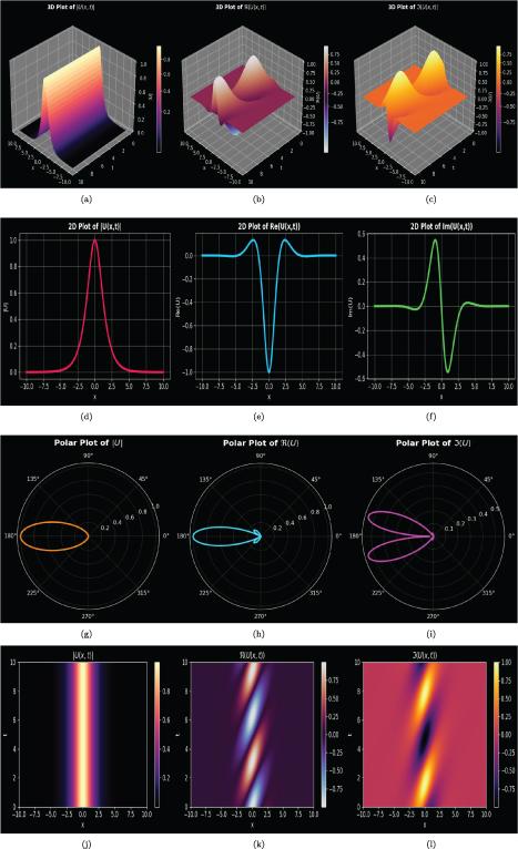
Figure 1. Three-dimensional surface plots, two-dimensional profiles, contour plots, polar plots of the bright optical soliton solution for $U(x,t)$. Real part, imaginary part, absolute value of $U(x,t)$ are shown to reveal the local structure, oscillations, and amplitude distribution of the solution, establishing its stability. |
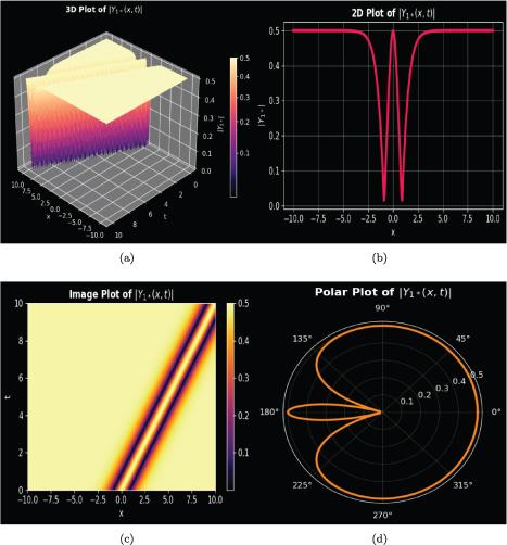
Figure 2. Visualization of the associated field $Y(x,t)$ through surface, profile, contour, and polar representations. The plots demonstrate the evolution of the localized bright-dark wave pattern and highlight the bounded behavior of the field component. |
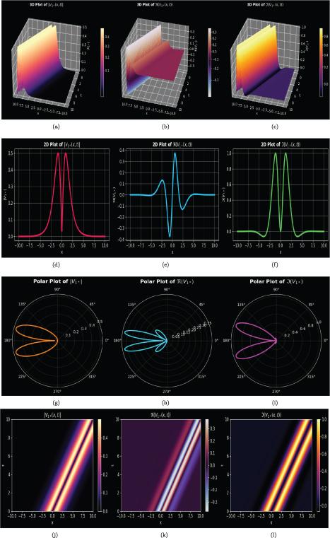
Figure 3. Surface, profile, contour, and polar representations of the field $V(x,t)$. The real part, imaginary part, and magnitude highlight phase oscillations, intensity variations, and the dynamical features associated with the higher-order field component. |
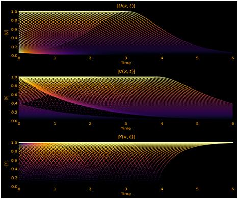
Figure 4. The superposition of the normalized intensity profiles yields the following temporal overlap patterns: $|U(x,t)|$, the magnitudes normalized by $|V(x,t)|$ and $|Y(x,t)|$ at different propagation times $t$. The repeated and overlapping profiles demonstrate that the profiles of the optical soliton along with its associated field components evolve in propagation in shape-preserving and stable manners. |
Figure 1 gives a full view of the bright optical soliton solution $U(x,t)$ with three-dimensional surface plots, two-dimensional profiles, contour maps and polar representation of its real part, imaginary part and absolute value. It can be seen that the magnitude $|U(x,t)|$ has a well-localized $\operatorname{sech}$ (x)-shaped structure with a confirming evidence of a bright soliton nature of the solution. The three-dimensional plots indicate that the soliton keeps its amplitude unchanged and localization in space during propagation. It points out an effective balance between dispersion and nonlinearity. Real and imaginary parts develop an oscillatory mode due to the phase term related to optical carrier waves. Contour and polar plots show the symmetry and stability of soliton profile further.
In figure 2, the associated field $Y(x,t)$ is visualized using its absolute value in three-dimensional, two-dimensional, contour, and polar plots. For the selected parameters, $|Y(x,t)|$ displays a distinct dark–bright soliton structure due to the presence of localized variations in intensity. Such a feature originates from the derivative-dependent nature of $Y(x,t)$, entailing an effective amplification of spatial gradients of the mother soliton field. It can be observed that this structure is preserved along the direction of propagation; this proves that $Y(x,t)$ propagates in a stable and bounded way.
Figure 3 shows the real part, imaginary part, and absolute value of the higher-order field $V(x,t)$ for the same collection of graphical utilities. The obtained profiles indicate an evident dark–bright soliton structure, thus proving that higher-order contributions do not destroy the localized nature of the solution. Instead, the soliton structure persists with modified amplitude characteristics. The real and imaginary parts illustrate phase-related oscillations, while the absolute value indicates the bounded and localized nature of $V(x,t)$, further reinforcing the robustness of the higher-order soliton component.
Figure 4 depicts the temporal overlap (eye-like) patterns achieved by superposing the normalized intensity profiles $|U(x,t)|^2$ and the normalized magnitudes $|V(x,t)|$ and $|Y(x,t)|$ at various propagation times $t$. The high level of overlap that these profiles exhibit indicates that the soliton solutions propagate without any observable distortion or spreading. Such is indeed a characteristic that defines optical solitons, which verifies the stability of both the primary and the associated field components. Note well that this diagram represents a form of temporal overlap or eye-like pattern rather than a conventional digital eye diagram, since no discrete modulation is imposed.
In all, the graphical results from figures 1–4 confirm that the obtained solutions represent those stable optical solitons that exhibit bright and dark–bright characteristics depending on the considered field component. The consistency of the soliton profiles across multiple visualization techniques and propagation times validates the analytical solutions and highlights their relevance in nonlinear optical systems.
3. Dynamical behavior
The dynamical properties of the reduced system are of great importance to understanding the qualitative properties of the underlying nonlinear model. Furthermore, the development of solution trajectories, the stability of equilibrium points, and the emergence of different wave potentially relevant factors that could influence the, patterns are strongly influenced by the system parameters.
3.1. Bifurcation analysis
In order to study the influence of system parameter differences on the qualitative behavior of solutions, bifurcation analysis is carried out of the reduced dynamical system. By using the Galilean-type transformation, equation (17 ) can be written as 25 ) is
$\begin{align} \frac{\mathrm{d}U}{\mathrm{d}\zeta} &= Q, \nonumber\\ \frac{\mathrm{d}Q}{\mathrm{d}\zeta} &= A\,U\left(\zeta\right)^3 + B\,U\left(\zeta\right),\end{align}$
where $A = -2$ and $B = k^{2}+2\omega$. The corresponding Hamiltonian form of ( $\begin{align} H\left(U,Q\right) = \frac{1}{2} Q^2 - \frac{A}{4}U^{4} - \frac{B}{2}U^{2}.\end{align}$
The fixed points satisfy $\begin{equation*} Q = 0,\qquad U\left(AU^{2}+B\right) = 0.\end{equation*}$
Thus the equilibria are $\begin{equation*} \left(U,Q\right) = \left(0,0\right), \qquad \left(U,Q\right) = \left(\pm \sqrt{-\frac{B}{A}},\,0\right),\end{equation*}$
whenever $-\frac{B}{A} \gt 0$. Since $A = -2 \lt 0$, the nontrivial points exist only when $B \gt 0$. The Jacobian of the system is $\begin{equation*} \boldsymbol{J} = \begin{pmatrix} 0 & 1 \\ 3AU^{2}+B & 0 \end{pmatrix}, \qquad \lambda^{2} = 3AU^{2}+B.\end{equation*}$
We classify the equilibria case by case.
Case 1: $B \gt 0$
Equilibria:
$\begin{equation*} \left(0,0\right),\qquad \left(\pm\sqrt{-\frac{B}{A}},0\right) = \left(\pm\sqrt{\frac{B}{2}},0\right).\end{equation*}$
• At the origin $(0,0)$:
$\begin{equation*} \lambda^{2} = B \gt 0,\end{equation*}$
so the origin is a saddle point.• At the nonzero equilibria:
$\begin{equation*} \lambda^{2} = 3A\left(\frac{B}{2}\right)+B = -3B + B = -2B \lt 0,\end{equation*}$
so these two points are centers.Thus the phase portrait contains a saddle at the origin and two centers symmetrically located on the $U$-axis as shown in figure 5.
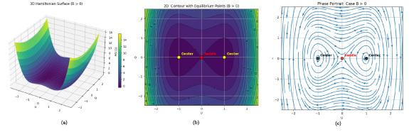
Figure 5. Phase portraits and Hamiltonian structure for the case $B \gt 0$. (a) The phase portrait shows that the origin is a saddle, while two additional equilibrium points appear symmetrically on the $U$-axis, both of which are centers. (b) The corresponding 3D Hamiltonian surface illustrates the saddle geometry at the origin and the elliptic wells around the centers. (c) The 2D contour plot of the Hamiltonian confirms the saddle at the origin and the closed contours surrounding the two center equilibria. |
Case 2: $B = 0$
Equilibria reduce to
$\begin{equation*} \left(U,Q\right) = \left(0,0\right).\end{equation*}$
Here,
$\begin{equation*} \lambda^{2} = 0,\end{equation*}$
so the origin becomes a center-type degenerate equilibrium. This case corresponds to the pitchfork bifurcation point where the two nontrivial equilibria collide with the origin as shown in figure 6.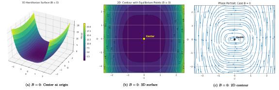
Figure 6. Phase portraits and Hamiltonian structure for the case $B = 0$. At this critical value, a pitchfork bifurcation occurs. The only equilibrium is the origin, which becomes a degenerate center. (a) The phase portrait exhibits neutrally stable center-type behavior. (b) The 3D Hamiltonian surface shows the flattening of the potential near the origin. (c) The 2D contour plot reflects circular level sets corresponding to the center-type equilibrium. |
Case 3: $B \lt 0$
Only one equilibrium exists:
$\begin{equation*} \left(U,Q\right) = \left(0,0\right).\end{equation*}$
Since
$\begin{equation*} \lambda^{2} = B \lt 0,\end{equation*}$
the origin is a center. The contours reveal closed orbits corresponding to bounded periodic-type solutions as given in figure 7.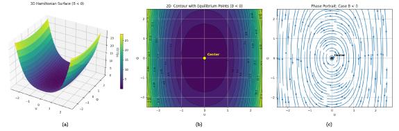
Figure 7. Phase portraits and Hamiltonian structure for the case $B \lt 0$. In this regime, the origin becomes a stable center and closed periodic orbits surround it. No nontrivial equilibrium points exist. (a) The phase portrait depicts the center at the origin with surrounding closed trajectories. (b) The 3D Hamiltonian surface forms a single elliptic potential well. (c) The 2D contour plot shows nested closed contours corresponding to bounded periodic-type solutions. |
3.2. Chaotic dynamics analysis
To investigate the chaotic behavior of the proposed dynamical system, we consider the perturbed Hamiltonian system [32, 33] solve_ivp routine in Python. The system was solved over the interval $\zeta \in [0,200]$ with a fixed time step $\Delta \zeta = 0.05$, which was verified to provide stable and convergent results.
$\begin{align} \frac{\mathrm{d}U}{\mathrm{d}\zeta} & = Q, \nonumber\\ \frac{\mathrm{d}Q}{\mathrm{d}\zeta} & = A U^{3} + B U + \delta \sin\left(\nu \zeta\right),\end{align}$
where $A = -2$, $B$ is the linear stiffness parameter, $\delta$ denotes the forcing amplitude, and $\nu$ represents the excitation frequency. The inclusion of the periodic forcing term breaks the integrability of the system and gives rise to rich nonlinear and chaotic dynamics. To ensure reproducibility and numerical accuracy, the reduced dynamical system was integrated using a fourth-order Runge–Kutta method implemented via the To eliminate transient effects, the initial portion of the solution ($\zeta \lt 100$) was discarded, and all dynamical quantities were computed using the remaining steady-state data. For the Poincaré Sections, intersections were sampled at discrete times corresponding to integer multiples of the excitation period $T = \frac{2\pi}{\nu}$ after transient removal.
Case I: $\nu = 1$
Figure 8 illustrates the dynamical behavior of the system for different values of the parameters $\delta$ and $B$ with the forcing frequency fixed at $\nu = 1$. Panels (a), (d), and (g) depict the two-dimensional phase portraits $(U,Q)$, panels (b), (e), and (h) show the corresponding time series of $U(\zeta)$, while panels (c), (f), and (i) present the associated Poincaré sections.
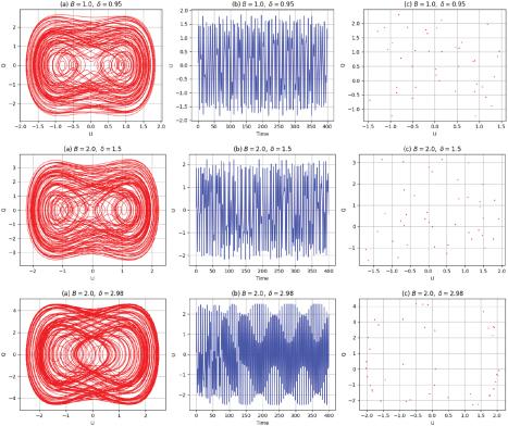
Figure 8. Phase Plots, Times Series and Poincare plots for case 1,showing chaos analysis. |
For smaller values of $\delta$, the phase trajectories form regular closed curves, indicating periodic motion. As $\delta$ increases, the phase portraits become increasingly distorted, the time series exhibit irregular oscillations, and the Poincaré sections evolve from isolated points to scattered sets, confirming the onset of chaotic behavior.
Case II: $\nu = \pi$
In figure 9, the excitation frequency is increased to $\nu = \pi$ while keeping different combinations of $\delta$ and $B$. Compared with the previous case, the phase portraits display stronger deformation and the time series reveal more complex amplitude modulations. The corresponding Poincaré sections show a denser distribution of points, indicating an enhancement of chaotic dynamics due to the increase in the forcing frequency.
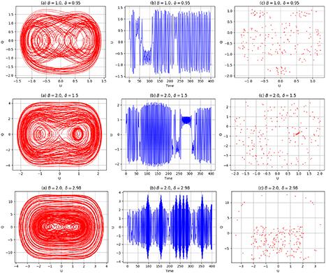
Figure 9. Phase Plots, Times Series and Poincare plots for case 2,showing chaos analysis. |
Case III: $\nu = 3\pi$
Figure 10 presents the system dynamics for $\nu = 3\pi$ and varying values of $\delta$ and $B$. In this high-frequency regime, the phase space is dominated by irregular trajectories filling a broad region, the time series becomes highly aperiodic, and the Poincaré sections form widely scattered point clouds. These features clearly demonstrate fully developed chaotic motion.
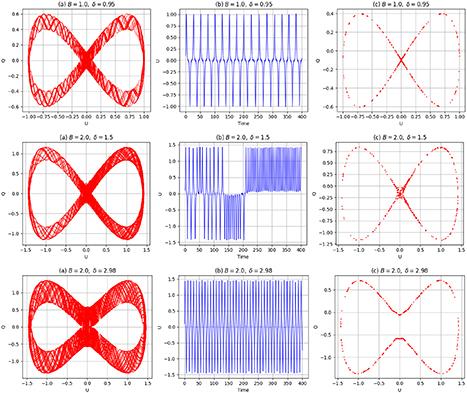
Figure 10. Phase Plots, Times Series and Poincare plots for case 3,showing chaos analysis. |
Overall, the numerical results confirm that the combined effects of the forcing amplitude $\delta$, the system parameter $B$, and the excitation frequency $\nu$ play a crucial role in governing the transition from periodic to chaotic dynamics in the proposed system.
3.2.1. Multistability analysis.
Multistability refers to the coexistence of multiple stable states for a given set of system parameters. In this study, we analyze the multistable behavior of the system by examining its phase-plane trajectories for different initial conditions and forcing parameters.
The system was solved numerically using the solve_ivp function in Python with several initial conditions:
$\begin{align*} \left[0.1, 0.0\right], \quad \left[0.5, 0.0\right], \quad \left[1.0, 0.0\right], \quad \left[-0.5, 0.0\right].\end{align*}$
Two representative values of $\delta$ ($2$ and $0.05$) and three values of $\nu$ ($1, \pi, 3\pi$) were considered to explore the effect of external forcing. The solutions were visualized in the $U$–$Q$ phase plane.
Figures 11 show the phase portraits of the system under different combinations of $\delta$ and $\nu$. Each trajectory corresponds to a distinct initial condition. It is evident that:
| • For higher forcing amplitude ($\delta = 2$), the system trajectories diverge more significantly, indicating stronger sensitivity to initial conditions and more pronounced multistability. | |
| • For lower forcing amplitude ($\delta = 0.05$), the trajectories are closely grouped, suggesting weaker multistability. | |
| • Variation of the forcing frequency ($\nu = 1, \pi, 3\pi$) alters the trajectory shapes and separations, reflecting the impact of external periodic forcing on the coexistence of multiple states. |
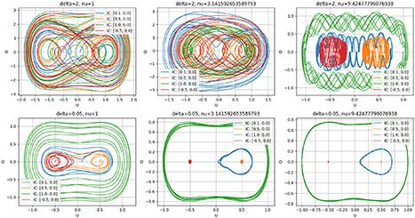
Figure 11. Phase portraits showing multistability for different values of $\delta$ and $\nu$. Each trajectory corresponds to a different initial condition. |
The legend in each plot identifies the initial conditions corresponding to each trajectory, highlighting the dependence of the system’s long-term behavior on the starting point.
Overall, the numerical results confirm that the system exhibits multistable dynamics, and the number and type of coexisting states are strongly influenced by the parameters $\delta$ and $\nu$ as shown in figure 11.
3.2.2. Sensitivity analysis.
Sensitivity analysis investigates how small changes in initial conditions or system parameters affect the behavior of the system. We numerically integrate the system and visualize the results with the following figures:
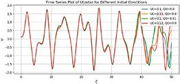
Figure 12. Time series plots of $U(\zeta)$ for slightly different initial conditions, illustrating the sensitivity of the system to initial perturbations. |
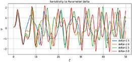
Figure 13. Parameter sensitivity analysis showing the evolution of $U(\zeta)$ for different values of $\delta$. Small changes in $\delta$ significantly affect the system response. |
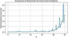
Figure 14. Divergence of trajectories for two close initial conditions, showing how the distance between trajectories grows over time. This highlights the system’s sensitive dependence on initial conditions. |
3.2.3. Some other properties of chaos analysis.
Recurrence plots
To further investigate the sensitivity and nonlinear characteristics of the system, recurrence plots are employed for the state variables $U(\zeta)$ and $Q(\zeta)$. Recurrence plots provide a qualitative visualization of recurring states in the system’s evolution and are particularly effective in identifying periodicity, quasi-periodicity, and irregular dynamics.
The recurrence patterns in figure 15 reveal variations in temporal structures, confirming that small perturbations in the system lead to significant changes in its evolution.
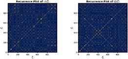
Figure 15. Recurrence plots for (left) $U(\zeta)$ and (right) $Q(\zeta)$. The complex and nonuniform recurrence structures indicate sensitive dependence on initial conditions and nonlinear dynamics. |
Power spectrum analysis
To further analyze the dynamical characteristics of the system, the power spectra of the variables $U(\zeta)$ and $Q(\zeta)$ are examined. The power spectrum reveals the dominant frequencies present in the system and helps distinguish between periodic, quasi-periodic, and broadband (irregular or chaotic) dynamics as given in figure 16.
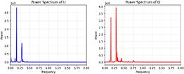
Figure 16. Power spectra of (left) $U(\zeta)$ and (right) $Q(\zeta)$. The presence of broadband components indicates complex and sensitive dynamical behavior. |
Bifurcation analysis via parameter variation
To examine the qualitative changes in the system dynamics, a bifurcation analysis is performed by varying the control parameter $\delta$ while keeping the remaining parameters fixed. The long-term behavior of the system is recorded after discarding transient effects. The bifurcation diagrams were constructed by varying the control parameter (e.g. $\delta$) incrementally and recording the asymptotic local maxima of $U(\zeta)$ over the steady-state interval. This procedure ensures that only long-term dynamical behavior is represented.
The figure 17 demonstrates that small variations in the bifurcation parameter can significantly alter the system response, confirming its sensitive nonlinear behavior.
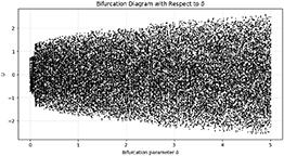
Figure 17. Bifurcation diagram of the system with respect to the parameter $\delta$. The emergence of multiple branches indicates transitions from regular to complex dynamics. |
Quantitative chaos verification via largest Lyapunov exponent
While qualitative indicators such as phase portraits, Poincaré sections, recurrence plots, and broadband power spectra suggest chaotic behavior, a quantitative confirmation is obtained by computing the largest Lyapunov exponent (LLE). The Lyapunov exponent measures the average exponential divergence of two initially close trajectories in phase space and provides a rigorous criterion for chaos. A positive value of the LLE indicates sensitive dependence on initial conditions and hence chaotic dynamics.
For the perturbed Hamiltonian system
$\begin{align} \frac{\mathrm{d}U}{\mathrm{d}\zeta} & = Q,\end{align}$
$\begin{align} \frac{\mathrm{d}Q}{\mathrm{d}\zeta} & = AU^3 + BU + \delta \sin\left(\nu \zeta\right),\end{align}$
the LLE was computed numerically using the standard renormalized Benettin algorithm. Two trajectories with an initial separation of order $10^{-8}$ were integrated simultaneously, and periodic renormalization was applied to maintain numerical stability. The Lyapunov exponent was evaluated as $\begin{equation} \lambda = \lim_{\zeta \to \infty} \frac{1}{\zeta} \ln \left( \frac{\mathrm{d}\left(\zeta\right)}{\mathrm{d}\left(0\right)} \right),\end{equation}$
where $\mathrm{d}(\zeta)$ denotes the Euclidean distance between the two trajectories in the $(U,Q)$ phase space.Figure 18 illustrates the convergence of the Largest Lyapunov Exponent as a function of $\zeta$. After an initial transient regime, the exponent stabilizes to a positive constant value,
$\begin{equation*} \lambda \approx 0.0293.\end{equation*}$
The positivity of the Lyapunov exponent quantitatively confirms the presence of chaotic dynamics in the system under the selected parameter set.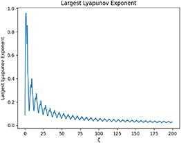


Figure 18. Largest Lyapunov exponent as a function of the evolution variable $\zeta$. The convergence toward a positive value ($\lambda \approx 0.0293$) confirms chaotic behavior. |
This result strengthens the qualitative chaos analysis presented earlier and provides rigorous numerical evidence of sensitive dependence on initial conditions.
4. Application
The analytical soliton solutions and the dynamical analysis of the SMB system provide insights into controllable wave propagation in resonant nonlinear media. Such results are relevant to optical fiber communication, laser pulse propagation, nonlinear photonic devices, and optical signal processing. In addition, the investigation of bifurcation, multistability, and chaotic dynamics can contribute to applications in secure optical communication, random signal generation, and stability control of nonlinear optical systems. However, the analytical and numerical results obtained in this work have extensive applications in nonlinear optics and photonics due to the fact that optical solitons can be controlled, manipulated, and utilized. Exact soliton solutions, bright, dark, and complex structures, directly apply to high-speed fiber-optic communication systems in which soliton stability and robustness are at a premium for long-distance data transmission with at most minimal signal degradation. Temporal overlaps and the interaction of the solitons will provide system designers with an understanding of how to do pulse shaping, dispersion management, and synchronization of signals to improve efficiency and reliability in optical networks.
From a practical point of view, chaotic dynamics, multistability, and sensitivity to initial conditions may be investigated in laser systems and nonlinear photonic devices. Such findings allow one to precisely tune system parameters, either to avoid undesired chaotic behaviors or to exploit controlled chaos in applications such as secure optical communication, encryption, and random number generation. Recurrence plots and power spectrum analyses provide effective tools for monitoring soliton dynamics, predicting instabilities, and designing adaptive control mechanisms for optical devices.
These rich dynamical behaviors described in the present study, such as bifurcation phenomena and multistability, can be exploited in all-optical switches, logic gates, and signal routers. Such ultrafast information processing devices rely on nonlinear wave propagation and controllable interactions of solitons. In high-power applications of lasers, such knowledge of parameter regimes that lead to stable formation of solitons can prevent the breakup of pulses or catastrophic instabilities that may occur to ensure reliable operation of laser amplifiers, optical pulse compressors, and nonlinear frequency converters.
The same understanding applies directly to new photonic devices, like optical sensors, photonic crystals, and integrated optics, where careful soliton management can lead to improvements in sensitivity, stability, and performance. By combining the exact solution of optical solitons with dynamical analysis, this work offers a general framework that allows an explanation and an exploitation of soliton dynamics in real optical and photonic systems. Future work may extend the present study to higher-dimensional SMB models, fractional-order formulations, and stochastic effects to further explore complex nonlinear wave interactions and their applications in advanced optical and photonic systems. The physical interpretation and applications of the graphical results are also given in table 1.
Table 1. Physical interpretation and applications of the graphical results. |
| Graph type | Physical interpretation | Potential applications |
|---|---|---|
| Absolute value $|U(x,t)|$ | Represents the intensity profile of the optical pulse and shows the localization and stability of the soliton structure. | Optical fiber communication, pulse transmission, and signal stability analysis. |
| Real part $\Re(U(x,t))$ | Describes the physical waveform of the propagating field and illustrates oscillatory behavior due to the carrier wave. | Wave propagation analysis, laser pulse dynamics, and optical signal modulation. |
| Imaginary part $\Im(U(x,t))$ | Shows the phase-related component of the complex field and helps understand phase evolution during propagation. | Phase control in photonic devices and coherent optical systems. |
| Contour plots | Illustrate the spatial distribution and localization of wave energy in the propagation domain. | Visualization of wave localization in nonlinear optical media. |
| Polar plots | Represent amplitude distribution in polar coordinates and reveal symmetry and structural stability of the soliton. | Analysis of wave symmetry and stability in nonlinear systems. |
| Phase portraits $(U,Q)$ | Describe the dynamical behavior of the reduced system and identify equilibrium points and trajectories. | Stability analysis of nonlinear dynamical systems. |
| Poincaré sections | Provide cross-sectional views of trajectories to identify periodic or chaotic motion. | Chaos detection in nonlinear optical and physical systems. |
| Bifurcation diagrams | Show how system behavior changes as parameters vary and identify transitions between periodic and chaotic regimes. | Parameter control and stability optimization in nonlinear photonic systems. |
| Lyapunov exponent plot | Quantifies sensitivity to initial conditions and confirms chaotic dynamics. | Secure communication, random signal generation, and nonlinear control systems. |
In all, the findings contribute to basic research in nonlinear wave dynamics and provide a practical basis for technology development that could enable the next generation of optical communication networks, laser systems, and other advanced photonic devices.
5. Conclusion
In this work we have presented a comprehensive analytical and numerical investigation of optical soliton dynamics in a (1+1)-dimensional nonlinear system. We applied the new Kudryashov’s method to obtain exact soliton solutions, bright, dark, and complex localized structures, and offered detailed graphical representations with the help of 3D, 2D, contour, and polar plots. The temporal overlap analysis conducted thereafter unraveled interaction and evolution characteristics of the solitons, and gave a major indication of the stability and robustness of the obtained solitons under different system parameters. The nonlinear dynamical behavior of the system was also investigated in the present study. Through a bifurcation analysis, it is presented how variations in key parameters of the system can lead to jumps between stability and instability. Chaotic dynamics, multistability, and sensitivity to initial conditions were all revealed by numerical simulations, while recurrence plots and power spectrum analysis provided insight into the temporal and frequency domain behavior of the solitons. These investigations point out the rich and intricate dynamics inherent in nonlinear optical systems. In this way, the obtained results of this research provide not only exact solutions and an advanced understanding of the behavior of solitons but also very important insights into practical applications in fiber optics, laser systems, and nonlinear photonics, where controlled soliton propagation and manipulation are required. Future studies can be extended by considering problems within higher-dimensional systems, taking stochastic effects into consideration, or even fractional-order models in order to further examine the complex interaction of solitons and their technological applications.
Data availability statement
All the data used during this study is accessible within the manuscript.
Ethical approval
The authors affirm their commitment to ethical standards.
Conflict of interest
There is no conflicts of interest to declare.
Funding
The authors received no financial support for the research and publication of this article.