Welcome to visit Communications in Theoretical Physics,
Mathematical Physics

Riccati sub-equation neural networks method for exact solutions of partial differential equations

  • Mengke Yu 1, 2 ,
  • Jiawei Wang 1 ,
  • Yanqin Liu , 2, * ,
  • Xiaoxue Zhang 2 ,
  • Runfa Zhang 3 ,
  • Libo Feng 4
Expand
  • 1School of Mathematics and Statistics, Qilu University of Technology (Shandong Academy of Sciences), Jinan 250353, China
  • 2School of Mathematics and Big Data, Dezhou University, Dezhou 253023, China
  • 3School of Automation and Software Engineering, Shanxi University, Taiyuan 030013, China
  • 4School of Mathematical Sciences, Queensland University of Technology, GPO Box 2434, Brisbane, Qld. 4001, Australia

*Author to whom any correspondence should be addressed.

Received date: 2026-02-03

  Revised date: 2026-06-07

  Accepted date: 2026-06-09

  Online published: 2026-07-15

Copyright

© 2026 Institute of Theoretical Physics CAS, Chinese Physical Society and IOP Publishing. All rights, including for text and data mining, AI training, and similar technologies, are reserved.
This article is available under the terms of the IOP-Standard License.

Abstract

Neural networks, with their high expressiveness in function approximation, have become an important research area for finding exact solutions of partial differential equations (PDEs). This paper employs a neural network-based analytical solutions (NNAS) method, which uses explicit neural networks models as trial functions for PDEs. By substituting the trial functions into the PDEs and solving the resulting algebraic systems symbolically, exact solutions can be obtained. However, this method requires designing specific activation functions for each problem, which often limits the diversity of solutions. To overcome this limitation, this paper extends the Riccati sub-equation neural networks (RSENNs) framework by using different solution forms of the Riccati equation as activation functions in the first hidden layer, and constructing trial functions through feedforward computation. Compared with the NNAS method, the RSENNs method employs the Riccati solutions family as a unified activation function library, reducing the time required for the complex derivation of activation functions. To verify the effectiveness of this approach, the method is applied to the Burgers equation, Fokker–Planck equation, and KdV–mKdV equation, obtaining various solutions forms, including generalized interaction solutions, generalized rational function solutions, and generalized hyperbolic function solutions. These solutions correspond to wave interaction, singular behavior, and localized structures in nonlinear systems, demonstrating the advantages of the method in solutions diversity. Compared with the NNAS method, the RSENNs method also reduces the time required to find suitable activation functions and improves the efficiency of solving PDEs. This work represents an extension and further development of the RSENNs method, providing an effective approach for finding exact solutions to PDEs based on neural networks.

Cite this article

Mengke Yu , Jiawei Wang , Yanqin Liu , Xiaoxue Zhang , Runfa Zhang , Libo Feng . Riccati sub-equation neural networks method for exact solutions of partial differential equations[J]. Communications in Theoretical Physics, 2026 , 78(9) : 095004 . DOI: 10.1088/1572-9494/ae7a04

1. Introduction

Partial differential equations (PDEs) play a crucial branch of mathematics, often used to describe and explain complex phenomena, holding significant importance in physics [1] and engineering [2, 3]. For instance, the study of fluid dynamics [4], heat conduction [5], elastic mechanics [6, 7], and plasma physics [811] all rely on the theories and knowledge of PDEs for theoretical support. However, despite the widespread applications of PDEs across various disciplines, obtaining their exact solutions remains a challenging task.
The study of exact solutions to PDEs has not only propelled the development of fundamental mathematics but also provided key tools for modeling in physics, engineering, finance, and other fields. In recent years, significant progress has been made in the exploration of exact solutions to PDEs. Researchers have developed a diverse array of methods, such as the modified homotopy perturbation method [12, 13], the extended modified auxiliary equation mapping method [14], the Sardar sub-equation method [15, 16], and the $\frac{G^{^{\prime}}}{G}$-expansion method [17, 18]. The flourishing of these methodologies has profoundly advanced the field, offering valuable theoretical insights and powerful computational tools for solving PDEs.
In recent years, Zhang et al [19, 20] proposed the bilinear neural networks method (BNNM), marking the first application of neural networks techniques for obtaining exact analytical solutions to PDEs and filling a gap in artificial intelligence applications for exact solution derivation. This method integrates neural networks with symbolic computation, making BNNM a generally applicable approach for solving exact analytical solutions to nonlinear PDEs (NLPDEs) in certain contexts. Subsequently, Qasim et al [21] employed bilinear neural networks technology to investigate the (3+1)-dimensional Bateman–Burgers equation, successfully obtaining its interaction solutions and periodic type-I solutions. During the same period, Nguyen and Meesad [22] utilized bilinear neural networks technology based on Hirota’s bilinear form to solve the Benney–Luke equation. By selecting appropriate activation functions, they effectively derived various exact analytical solutions for this equation. Liu et al [23] embedded the $ \frac{G^{^{\prime}}}{G} $-expansion method into the neural networks framework, pioneering the $ \frac{G^{^{\prime}}}{G} $-expansion neural networks analytical method and successfully obtaining explicit exact solutions for NLPDEs. In addition, the neural network-based analytical solutions (NNAS) method [24] constructs explicit neural networks models as trial functions, which are then substituted into the target equations to derive systems of nonlinear algebraic equations for obtaining exact solutions. Mohammad et al [2528] proposed the Riccati sub-equation neural network (RSENNs) method, which employs the solutions of Riccati sub-equations as activation functions in neural networks architectures and demonstrates its effectiveness and applicability in obtaining exact solutions for NLPDEs.
Compared with existing neural network-based methods, such as the BNNM, the $ \frac{G^{^{\prime}}}{G} $-expansion neural networks method, and the NNAS method, these approaches differ in the construction of activation functions and the generation of solutions. In terms of activation function design, the BNNM, $ \frac{G^{^{\prime}}}{G} $-based methods, and the NNAS method generally relies on problem dependent constructions or predefined analytical forms, which require manual selection and prior knowledge of solutions structures. In contrast, the RSENNs method employs the solutions families of the Riccati equation as activation functions, providing a more systematic way to construct trial functions. Regarding the scope of solutions, the BNNM is mainly applicable to equations that can be transformed into bilinear forms, while the $ \frac{G^{^{\prime}}}{G} $-expansion method is limited to finite expansion structures. The NNAS method shows certain generality, but its solutions forms depend on the chosen activation functions. The original RSENNs method adopts a single solutions form of the Riccati equation and is therefore still limited in solutions diversity. In terms of computational efficiency, these methods often involve a lengthy and complex derivation process in designing activation functions. The RSENNs method alleviates this issue by standardizing the generation of activation functions, improving preprocessing efficiency to some extent.
Based on the above analysis and inspired by the trial functions construction mechanism in the NNAS method, this paper extends the RSENNs method by introducing a form selection strategy for Riccati solutions. By incorporating multiple functional forms (such as $\varphi$, $\varphi^2$, and $\frac{1}{\varphi}$), the proposed method enhances the flexibility of trial functions construction and improves its expressive capability.
Specifically, different solutions forms of the Riccati equation are selected based on the structural characteristics of the equations and are employed as activation functions in the first hidden layer of the neural networks. This strategy enables the construction of more flexible trial solutions forms and improves the adaptability of the method to some extent.
To demonstrate the applicability of the proposed method, it is applied to three typical NLPDEs, namely the Burgers equation, the Fokker–Planck equation, and the KdV–mKdV equation, which correspond to dissipative, diffusive, and dispersive physical processes, respectively. The main contributions of this work are summarized as follows,

• A form selection strategy for Riccati solutions is proposed, in which multiple forms are introduced as activation functions, thereby extending the conventional single form method.

• Various exact solutions for different types of NLPDEs are obtained, illustrating the applicability of the proposed method.

• The scope and limitations of the method are discussed, including its dependence on the solutions forms of the Riccati equation and the increased computational cost with networks complexity.

The structure of this paper is as follows. Section 2 introduces the main theoretical foundations, including the Riccati sub-equation method, the neural networks architecture, and the NNAS method [28]. Section 3 develops the RSENNs method based on the framework described in section 2. In particular, multiple solutions forms of the Riccati equation (including $\varphi$, $\varphi^2$, and $\frac{1}{\varphi}$) are embedded into the first hidden layer of the neural networks, and the implementation procedure of the extended RSENNs method is presented in detail. Section 4 considers the Burgers, Fokker–Planck, and KdV–mKdV equations as examples, and obtains their exact solutions using both the NNAS method and the RSENNs method. Section 5 provides a comparison between the two methods, along with further discussion. Finally, the conclusions of this paper are presented in section 6.

2. Preliminaries

In this section, we will introduce the main relevant theories of this paper, including the Riccati sub-equation method, neural networks architecture, and the NNAS method, to lay a solid theoretical foundation for RSENNs. For a PDE with the following general form,
$\begin{equation} F\left(x_1,\dots,x_n,u,\frac{\partial u}{\partial x_1},\dots,\frac{\partial u}{\partial x_n},\frac{\partial^2 u}{\partial x_1\partial x_2},\dots,\frac{\partial^m u}{\partial x_n^m}\right) = 0,\end{equation}$
where $u$ is the unknown function, $x_1,x_2,x_3,\dots,x_n$ represent the independent variables, and the order $m$ of the highest-order partial derivative $\frac{\partial^m u}{\partial x_n^m}$ in the equation is called the order of the equation.

2.1. Riccati sub-equation method

As a mathematical modeling technique, the sub-equation [29] enables either derivation of exact solutions to PDEs or procedural simplification of their solution. This study specifically adopts the Riccati equation $\varphi^{^{\prime}} = \sigma+\varphi^2$ as the foundational sub-equation. When $\sigma$ takes different symbols, the specific solutions of the Riccati equation has been shown as follows,
$\begin{equation} \varphi\left(\xi\right) = \left\{\begin{array}{ll} -\sqrt{-\sigma} \tanh\left(\sqrt{-\sigma} \xi\right), & \sigma \lt 0, \\ -\sqrt{-\sigma} \operatorname{coth}\left(\sqrt{-\sigma} \xi\right), & \sigma \lt 0, \\ \sqrt{\sigma} \tan\left(\sqrt{\sigma} \xi\right), & \sigma \gt 0, \\ -\sqrt{\sigma} \cot\left(\sqrt{\sigma} \xi\right), & \sigma \gt 0, \\ -\frac{1}{\xi+\omega}. & \sigma = 0, \omega = \text {const. } \end{array}\right.\end{equation}$

2.2. Neural networks architecture

Neural networks [3032] are mathematical models that mimic biological nervous systems, obtaining trial functions for PDEs through their feedforward computations. The structure is as follows.
The input layer $L_0$ contains $n$ neurons, $w_{x_i,j}$ denotes the weight coefficient between neuron $x_i$ and neuron $\xi_{j}$ in the hidden layer $L_{1}$.$w_{k,s}$ represents the weight coefficient between neuron $\xi_{k}$ in the previous hidden layer and neuron $\xi_{s}$ in the next hidden layer.$F_k$ denotes the activation function for the corresponding neurons in this neural networks architecture. The output layer contains a single neuron $u$, where $w_{r,u}$ denotes the weight coefficient between neuron $\xi_{r}$ in the hidden layer $L_{m}$ and neuron $u$.
After the feedforward computation of the neural networks, the output function is
$\begin{align} u & = w_{n_{m-1}+1,u} F_{n_{m-1}+1}\left(\xi_{n_{m-1}+1}\right)+ w_{n_{m-1}+2,u} \nonumber\\ &\quad \times F_{n_{m-1}+2}\left(\xi_{n_{m-1}+2}\right) + \dots + w_{n_m,u} F_{n_m}\left(\xi_{n_m}\right). \end{align}$
According to the universal approximation theorem [33] and the multilayer feedforward theorem [34], neural networks can approximate any complex function with arbitrary precision. Their construction depends not only on the selection of nonlinear activation functions but more importantly on the structural form of multilayer neural networks and neurons. The expansion of neural networks theoretical foundations has laid a solid groundwork for future research across diverse fields.

2.3. Neural network-based analytical solutions method

The NNAS method for obtaining exact solutions of PDEs rely on the neural networks architecture, using its explicit model as trial function for the PDEs solutions. The steps of this method are as follows.

Step 1. Constructing a neural networks model by selecting specific activation functions, numbers of neurons, and numbers of hidden layers, and then using the feedforward computation of the network to obtain trial function for equation (1).

Step 2. Substituting the trial function into equation (1), combining like terms of the resulting algebraic expression, extracting the coefficients, and setting all coefficients to zero to generate an under-determined system of nonlinear algebraic equations.

Step 3. Owing to the complexity of solving the algebraic system, symbolic computation software (e.g. Maple) is employed to solve the equations and determine the values of some weights and biases.

Step 4. Substituting the obtained weights and bias coefficients back into the trial function from Step 1 to derive the exact solutions of equation (1).

Step 5. Verifying the correctness of the exact solutions by inserting them into equation (1) again to ensure they satisfy the equation.

Step 6. For different types of PDEs, adjusting the networks architecture and parameters and optimizing the form of the trial function to improve the applicability and accuracy of the solutions.

3. Riccati sub-equation neural networks
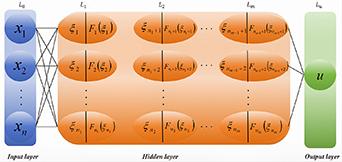
The RSENNs method employed in this section is based on the RSENNs framework proposed by Mohammad et al Motivated by the construction mechanism of the NNAS method and the process of activation function design, this study extends the original RSENNs approach by systematically exploring multiple solutions forms of the Riccati sub-equation, such as $\varphi$, $\varphi^2$, and $\frac{1}{\varphi}$, different forms are selected based on the characteristics of specific equations and embedded as activation functions in the neural networks architecture, enabling the derivation of exact solutions in a more diverse form. In this study, the neural networks architecture consists of two hidden layers, with each hidden layer containing two neurons. The networks architecture is chosen based on several commonly used functional forms, and these forms are tested to ensure the method’s effectiveness and reproducibility. The core idea of the RSENNs method consists of two main aspects. First, different solutions forms of the Riccati equation are used as activation functions in the hidden layers of the neural networks. Second, trial functions are substituted into the system of PDEs, transforming them into algebraic equations, which are then solved using symbolic computation software (such as Maple). The main steps of the proposed method are as follows.
Step 1. Selecting different solutions forms of the Riccati equation (2), such as $\varphi(\cdot)$, $\varphi(\cdot)^2$, $\frac{1}{\varphi(\cdot)}$, as activation functions for neurons in the first hidden layer of the neural networks model.
Step 2. Constructing the RSENNs model based on the activation functions chosen in Step 1. Except for the first hidden layer, the activation functions of all remaining hidden layers can be chosen flexibly according to the actual situation, and the trial function is obtained through forward computation. This neural networks model can be understood intuitively from figure 1.
Figure 1. Neural networks architecture diagram.
Step 3. Substituting the trial function obtained from Step 2 into the equation (1) to get an algebraic equation. Combining like terms in the resulting algebraic equation, extract all coefficients, and set each coefficient to zero to obtain an undetermined system of nonlinear algebraic equations. Solve these algebraic equations to obtain the coefficient solutions of weights and biases.
Step 4. Analyzing the obtained weights and biases, and based on the value of the parameter $\sigma$, selecting the specific form of the activation function according to (2) to derive the exact solutions of equation (1).
Step 5. Verifing the correctness of the obtained exact solutions by substituting them back into the original PDEs to ensure they satisfy the equation.
Step 6. For different forms of PDEs, adjusting the structure and parameters of the neural networks and optimizing the form of the trial function to improve the applicability and accuracy of the solutions.
By following the above steps, we can systematically obtain exact solutions of PDEs using neural networks models, thereby providing an effective tool for the analysis and solutions of complex physical problems. This method has significant advantages over the NNAS method, it offers an effective method for selecting activation functions, improves the efficiency of solving, and increases the variety of solutions.

4. Applications

In this section, we will focus on three types of PDEs, including the Burgers equation, the Fokker–Planck equation and KdV–mKdV equation. These problems will be solved using both the NNAS method and the RSENNs method.
We use the 2-2-2-1 NNAS model and RSENNs model, where the input layer and the two hidden layers are two neurons, and the output equation $u$ is the trial function for the solutions of PDEs. We have,
$\begin{align*}& \quad u = w_{3, u} F_{3}\left(\xi_{3}\right)+w_{4, u} F_{4}\left(\xi_{4}\right)+b_{5},\end{align*}$
$\begin{align} & \left\{\begin{array}{ll} \xi_{3} = w_{1,3} F_{1}\left(\xi_{1}\right)+w_{2,3} F_{2}\left(\xi_{2}\right)+b_{3},\nonumber\\ \xi_{4} = w_{1,4} F_{1}\left(\xi_{1}\right)+w_{2,4} F_{2}\left(\xi_{2}\right)+b_{4}, \nonumber\\ \xi_{1} = t w_{t, 1}+x w_{x,1}+b_{1}, \nonumber\\ \xi_{2} = t w_{t, 2}+x w_{x, 2}+b_{2}, \end{array}\right.\end{align}$
where $F_i(i = 1, 2, 3, 4)$ is the activation function, $w_{j,k}(j = x, t, 1, 2, 3, 4; k = 1, 2, 3, 4, u; j\neq k)$, and $b_l(l = 1, 2, 3, 4, 5)$ are real parameters that can be determined.

4.1. The Burgers equation

The Burgers equation is as follows,
$\begin{align} u\frac{\partial u}{\partial t} +\frac{\partial u}{\partial x} = \alpha\frac{\partial^2 u}{\partial x^2}, x\in\left[x_0,x_L\right], t\in\left[0,T\right].\end{align}$
where $\alpha$ is a constant.
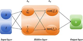
Case 1 The 2-2-2-1 NNAS model, defined in equation (4), is employed to construct exact solutions of the Burgers equation, as illustrated in figure 2. By specifying the activation functions as $F_1(\xi_{1}) = e{\xi_{1}}$, $F_2(\xi_{2}) = \frac{1}{\xi_{2}}$, $F_3(\xi_{3}) = \cot(\xi_{3})$, and $F_4(\xi_{4}) = \tan(\xi_{4})$, the reciprocal function $\frac{1}{(\cdot)}$ introduces rational and singular structures, while the trigonometric functions $\tan(\cdot)$ and $\cot(\cdot)$ are used to capture periodic behaviors, reflecting nonlinear wave patterns with repeating structures.
Figure 2. The 2-2-2-1 NNAS model of the Burgers equation.
The trial solution can be written as
$\begin{equation*}u = w_{3,u} \cot\left(\xi_{3}\right) + w_{4,u} \tan\left(\xi_{4}\right) + b_5.\end{equation*}$
The trial function $u(x,t)$ is
$\begin{align}u\left(x,t\right)& = \cot \! \bigg(\left(t w_{t ,1}+x w_{x ,1}+b_{1}\right) w_{1,3}\nonumber\\ &\quad +\frac{w_{2,3}}{t w_{t ,2}+x w_{x ,2}+b_{2}}+b_{3}\bigg) w_{3,u}\nonumber\\ &\quad +\tan \! \bigg(\bigg(t w_{t ,1}+x w_{x ,1}+b_{1}\bigg) w_{1,4}\nonumber\\ &\quad +\frac{w_{2,4}}{t w_{t ,2}+x w_{x ,2}+b_{2}}+b_{4}\bigg) w_{4,u}+b_{5}.\end{align}$
We substitute the trial function (6) into equation (5) and simplify the expression. By grouping similar terms based on combinations of
$\begin{align*} & \Big\{t, x, \cot \! \left(\left(t w_{t ,1}+x w_{x ,1}+b_{1}\right) w_{1,3}+\frac{w_{2,3}}{t w_{t ,2}+x w_{x ,2}+b_{2}}+b_{3}\right),\nonumber\\ &\quad\tan \! \left(\left(t w_{t ,1}+x w_{x ,1}+b_{1}\right) w_{1,4}+\frac{w_{2,4}}{t w_{t ,2}+x w_{x ,2}+b_{2}}+b_{4}\right)\Big\}, \end{align*}$
collecting the coefficients of each term and setting them to zero, we obtain an undetermined system of nonlinear algebraic equations. Using software Maple to solve this system of nonlinear algebraic equations, thirty sets of solutions can be obtained, which are not listed here one by one. The two solutions we finally choose are as follows.
Solution Set I
$\begin{align} \Big\{\alpha & = \alpha, b_{2} = 0, b_{5} = b_{5}, w_{1,3} = w_{1,3}, \nonumber\\ w_{1,4} & = w_{1,4}, w_{2,3} = w_{2,3}, w_{2,4} = 0,\nonumber\\ w_{3,u} & = 0, w_{4,u} = 2\alpha w_{1,4}w_{x,1}, w_{t,1} = -b_{5}w_{x,1}, \nonumber\\ w_{t,2} & = w_{t,2}, w_{x,1} = w_{x,1}, w_{x,2} = w_{x,2}\Big\}. \end{align}$
Solution Set II
$\begin{align} \Big\{\alpha& = \alpha, b_{2} = b_{2},b_{5} = b_{5}, w_{1,3} = w_{1,3}, \nonumber\\ w_{1,4}&= w_{1,4}, w_{2,3} = 0, w_{2,4} = w_{2,4},\nonumber\\ w_{3,u}&= -2\alpha w_{1,3}w_{x,1}, w_{4,u} = 0, w_{t,1} = -b_{5}w_{x,1},\nonumber\\ w_{t,2}&= 0, w_{x,1} = w_{x,1}, w_{x,2} = w_{x,2}\Big\}. \end{align}$
At this point, substituting solutions (7) and (8) into equation (6) yields two forms of the exact solutions
$\begin{align} u_{1}\left(x,t\right) & = 2 \tan \! (\left(-t b_{5} w_{x ,1}+x w_{x ,1}+b_{1}\right)\nonumber\\ &\quad\times w_{1,4}+b_{4}) \alpha w_{1,4} w_{x ,1}+b_{5}, \end{align}$
$\begin{align} u_{2}\left(x,t\right)& = -2 \cot \! (\left(-t b_{5} w_{x ,1}+x w_{x ,1}+b_{1}\right)\nonumber\\ &\quad\times w_{1,3}+b_{3}) \alpha w_{1,3} w_{x ,1}+b_{5}. \end{align}$
Taking equation (9) as an example, by selecting the coefficients
$\begin{align*} \Big\{w_{4, u} &= 3, w_{3,u} = 2, w_{x,1} = 10, w_{x,2} = 3, w_{t,1} = 2,\nonumber\\ & w_{t,2} = 4, w_{1,3} = 6, w_{1,4} = 7,\nonumber\\ & w_{2,3} = 1, w_{2,4} = 1, b_{1} = 1, b_{2} = 1,\nonumber\\ & b_{5} = 1, b_{3} = 1, b_{4} = 2, \alpha = 3\Big\}. \end{align*}$
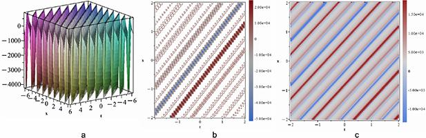
in equation (9), we obtain an exact periodic traveling wave solution to the Burgers equation. Its graphical representation is shown in figure 3, figure 3(a) presents a three-dimensional surface plot over the spatial-temporal domain $x \in [-2\pi, 2\pi], t \in [-2\pi, 2\pi]$, while figures 3(b) and (c) display the corresponding contour plot and density plot, respectively. This $\tan$-type solution exhibits periodic singularities at $70t - 70x - 9 = \frac{\pi}{2} + n\pi$, where it becomes unbounded. It represents a periodic traveling wave with phase velocity $c = 1$ and spatial period $T_x = \frac{\pi}{70}$. The resulting structure can be viewed as a periodic pattern of shock-like structures, characterized by rapidly varying gradients near the singular points, reflecting the nonlinear steepening mechanism of the Burgers equation.
Figure 3. The periodic traveling wave solution plot of the Burgers equation.
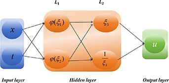
Case 2 The 2-2-2-1 RSENNs model, defined in equation (4), is employed to construct exact solutions of the Burgers equation, as illustrated in figure 4. By specifying the activation functions as $F_1(\xi_{1}) = \varphi(\xi_{1})$, $F_2(\xi_{2}) = \varphi(\xi_{2})$, $F_3(\xi_{3}) = \xi_{3}$, and $F_4(\xi_{4}) = \frac{1}{\xi_{4}}$, where $\varphi(\cdot)$ denotes a solution of the Riccati equation given in equation (2), the Riccati-based activation function $\varphi(\cdot)$ provides a systematic way to generate diverse functional forms. In particular, depending on the parameter choices, it can produce trigonometric-type and hyperbolic-type structures, which are associated with periodic and localized wave patterns, respectively. Meanwhile, the reciprocal function $\frac{1}{(\cdot)}$ introduces rational and singular structures into the solution.
Figure 4. The 2-2-2-1 RSENNs model of the Burgers equation.
The trial solution can be written as
$\begin{equation*}u = w_{3,u} \xi_{3} + w_{4,u} \frac{1}{\xi_{4}} + b_5.\end{equation*}$
The trial function $u(x,t)$ is
$\begin{align} u\left(x,t\right)& = w_{3,u} \left(w_{1,3} \varphi \! \left(t w_{t ,1}+x w_{x ,1}+b_{1}\right)+w_{2,3} \varphi \! \left(t w_{t ,2}+x w_{x ,2}+b_{2}\right)+b_{3}\right)\nonumber\\ &\quad +\frac{w_{4,u}}{w_{1,4} \varphi \! \left(t w_{t ,1}+x w_{x ,1}+b_{1}\right)+w_{2,4} \varphi \! \left(t w_{t ,2}+x w_{x ,2}+b_{2}\right)+b_{4}}+b_{5}. \end{align}$
We substitute the trial function (11) into equation (5) and simplify the expression, where $\varphi^{^{\prime}} = \sigma + \varphi^2$. By grouping similar terms based on combinations of $t$, $x$, $\varphi \! \left(t w_{t ,1}+x w_{x ,1}+b_{1}\right)$, $\varphi \! \left(t w_{t ,2}+x w_{x ,2}+b_{2}\right)$, then setting the coefficients of each term to zero, we ultimately obtain an undetermined system of nonlinear algebraic equations. This nonlinear system is subsequently solved using the symbolic computation software Maple, thirty sets of solutions can be obtained, which are not listed one by one here. The one solution we finally choose is as follows,
$\begin{align} \Big\{\alpha &= \alpha, \sigma = \sigma, b_{3} = b_{3}, b_{4} = b_{4}, b_{5} = b_{5},\nonumber\\ w_{1,3} &= 0, w_{1,4} = w_{1,4}, w_{2,3} = 0, w_{2,4} = 0, w_{3,u} = w_{3,u},\nonumber\\ w_{4,u} &= -\frac{2\alpha w_{x,1}\left(\sigma w_{1,4}^2 + b_{4}^2\right)}{w_{1,4}},\nonumber\\ w_{t,1} &= \frac{w_{x,1}\left(2\alpha b_{4}w_{x,1} - b_{3}w_{1,4}w_{3,u} - b_{5}w_{1,4}\right)}{w_{1,4}},\nonumber\\ w_{t,2} &= w_{t,2}, w_{x,1} = w_{x,1}, w_{x,2} = w_{x,2}\Big\}.\end{align}$
At this stage, by substituting solutions (12) into the equation (11) and considering the value of $\sigma$, we can obtain the following forms of exact solutions for the Burgers equation
$\begin{align}u\left(x,t\right) = b_{3} w_{3,u}-\frac{2 \alpha w_{x ,1} \left(\sigma w_{1,4}^{2}+b_{4}^{2}\right)}{w_{1,4} \left(w_{1,4} \varphi \! \left(\frac{t w_{x ,1} \left(2 \alpha b_{4} w_{x ,1}-b_{3} w_{1,4} w_{3,u}-b_{5} w_{1,4}\right)}{w_{1,4}}+x w_{x ,1}+b_{1}\right)+b_{4}\right)}+b_{5}. \end{align}$
When $\sigma \gt 0$,
$\begin{align}u_{1}\left(x,t\right)& = b_{3} w_{3,u}-\frac{2 \alpha w_{x ,1} \left(\sigma w_{1,4}^{2}+b_{4}^{2}\right)}{w_{1,4} \left(w_{1,4} \sqrt{\sigma}\, \tan \! \left(\sqrt{\sigma}\, \xi_{1}\right)+b_{4}\right)}+b_{5},\end{align}$
$\begin{align}u_{2}\left(x,t\right) & = b_{3} w_{3,u}-\frac{2 \alpha w_{x ,1} \left(\sigma w_{1,4}^{2}+b_{4}^{2}\right)}{w_{1,4} \left(-w_{1,4} \sqrt{\sigma}\, \cot \! \left(\sqrt{\sigma}\, \xi_{1}\right)+b_{4}\right)}+b_{5}, \end{align}$
where $\alpha$ is a constant, $\xi_{1} = \frac{t w_{x ,1} \left(2 \alpha b_{4} w_{x ,1}-b_{3} w_{1,4} w_{3,u}-b_{5} w_{1,4}\right)}{w_{1,4}}+x w_{x ,1}+b_{1}$.
When $\sigma \lt 0$,
$\begin{align}u_{3}\left(x,t\right)& = b_{3} w_{3,u}\nonumber\\ &\quad-\frac{2 \alpha w_{x ,1} \left(\sigma w_{1,4}^{2}+b_{4}^{2}\right)}{w_{1,4} \left(-w_{1,4} \sqrt{-\sigma}\, \tanh \! \left(\sqrt{-\sigma}\, \xi_{1} \right)+b_{4}\right)}+b_{5}, \end{align}$
$\begin{align}u_{4}\left(x,t\right) & = b_{3} w_{3,u}\nonumber\\ &\quad-\frac{2 \alpha w_{x ,1} \left(\sigma w_{1,4}^{2}+b_{4}^{2}\right)}{w_{1,4} \left(-w_{1,4} \sqrt{-\sigma}\, \coth \! \left(\sqrt{-\sigma}\, \xi_{1} \right)+b_{4}\right)}+b_{5}, \end{align}$
where $\alpha$ is a constant, $\xi_{1} = \frac{t w_{x ,1} \left(2 \alpha b_{4} w_{x ,1}-b_{3} w_{1,4} w_{3,u}-b_{5} w_{1,4}\right)}{w_{1,4}}+x w_{x ,1}+b_{1}$.
When $\sigma = 0$,
$\begin{align} u_{5}\left(x,t\right) = b_{3} w_{3,u}-\frac{2 \alpha w_{x ,1} \left(\sigma w_{1,4}^{2}+b_{4}^{2}\right)}{w_{1,4} \left(-\frac{w_{1,4}}{\xi_{1}+\omega}+b_{4}\right)}+b_{5}, \end{align}$
where $\omega$ and $\alpha$ are a constants, $\xi_{1} = \frac{t w_{x ,1} \left(2 \alpha b_{4} w_{x ,1}-b_{3} w_{1,4} w_{3,u}-b_{5} w_{1,4}\right)}{w_{1,4}}+x w_{x ,1}+b_{1}$.
Taking equation (16) as an example, by selecting the coefficients
$\begin{align*} &\Big\{w_{4, u} = 1, w_{3,u} = 2, w_{x,1} = 1, w_{x,2} = 2, w_{t,1} = 2,\\ &\quad w_{t,2} = 4, w_{1,3} = 6, \\ &\quad w_{1,4} = 7, w_{2,3} = 1, w_{2,4} = 1, b_{1} = 1, b_{2} = 1,\\ &\quad b_{5} = 1, b_{3} = 1, b_{4} = 1, \sigma = 3, \alpha = 1\Big\}, \end{align*}$
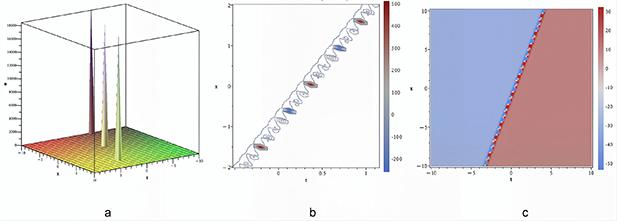
this gives an exact kink-type traveling wave solution to the Burgers equation is obtained. The graphical representation is shown in figure 5, figure 5(a) displays a three-dimensional surface plot over the spatial-temporal domain $x \in [-10, 10], t \in [-10, 10]$, while figures 5(b) and (c) present the corresponding contour plot and density plot, respectively. This $\tanh$-type solution represents a viscous shock wave propagating with velocity $c = \frac{19}{7}$. It exhibits a steep but continuous transition between two asymptotic states, reflecting the balance between nonlinear convection and viscous dissipation. The resulting profile corresponds to a viscous shock structure with finite thickness, which is a characteristic feature of Burgers-type systems.
Figure 5. The kink-type traveling wave solution plot of the Burgers equation.

4.2. The Fokker–Planck equation

The Fokker–Planck equation is as follows,
$\begin{align} \frac{\partial u\left(x,t\right)}{\partial t}& = -\frac{\partial}{\partial x}\left(T_1\left(x,t\right)\cdot u\left(x,t\right)\right)\\ &\quad +\frac{\partial^2}{\partial x^2}\left(T_2\left(x,t\right)\cdot u\left(x,t\right)\right),\\ &\quad x\in\left[x_0,x_L\right], t\in\left[0,T\right].\end{align}$
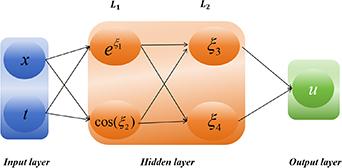
Case 1 The 2-2-2-1 NNAS model, defined in equation (4), is employed to construct exact solutions of the Fokker–Planck equation, as illustrated in figure 6. By specifying the activation functions as $F_1(\xi_{1}) = e^{\xi_{1}}$, $F_2(\xi_{2}) = \cos(\xi_{2})$, $F_3(\xi_{3}) = \xi_{3}$, and $F_4(\xi_{4}) = \xi_{4}$, the exponential function $e^{(\cdot)}$ introduces non-periodic growth behavior, while the cosine function $\cos(\cdot)$ captures oscillatory features, the identity mapping $(\cdot)$ preserves linear combinations of the transformed inputs.
Figure 6. The 2-2-2-1 NNAS model of the Fokker–Planck equation.
The trial solution can be written as
$\begin{align*} u = w_{3,u} \xi_{3} + w_{4,u} \xi_{4} + b_5.\end{align*}$
The trial function $u(x,t)$ is
$\begin{align}u\left(x,t\right)& =w_{3,u} (\mathrm{e}^{t w_{t ,1}+x w_{x ,1}+b_{1}} w_{1,3}\\ &\quad \times \cos \! \left(t w_{t ,2}+x w_{x ,2}+b_{2}\right) w_{2,3}+b_{3})\\ &\quad +w_{4,u} (\mathrm{e}^{t w_{t ,1}+x w_{x ,1}+b_{1}} w_{1,4} \\ &\quad \times \cos \! (t w_{t ,2}+x w_{x ,2}+b_{2}) w_{2,4}+b_{4})+b_{5}. \end{align}$
We substitute the trial function (20) into equation (19) and simplify the expression. By grouping similar terms based on combinations of $t$, $x$, $\varphi \! \left(t w_{t ,1}+x w_{x ,1}+b_{1}\right)$, $\varphi \! \left(t w_{t ,2}+x w_{x ,2}+b_{2}\right)$ collecting the coefficients of each term, and setting them to zero, we obtain an undetermined system of nonlinear algebraic equations. Using software Maple to solve this system of nonlinear algebraic equations, eight sets of solutions can be obtained, which are not listed one by one here. The one solution we finally choose is as follows,
$\begin{align} \left\{\begin{array}{ll} w_{t,1} = T_2w_{x, 1}^2 - T_2w_{x, 2}^2 - T_1w_{x, 1},\\ w_{t,2} = 2T_2w_{x, 1}w_{x, 2} - T_1w_{x, 2}, \end{array}\right.\end{align}$
at this point, substituting solutions (21) into equation (20) yields one form of the exact solutions
$\begin{align}u\left(x,t\right)& =\cos \! (((-2 T_{2} w_{x ,1}+T_{1}) t -x ) w_{x ,2}-b_{2}) \\ &\quad\times (w_{1,3} w_{2,3} w_{3,u}+w_{1,4} w_{2,4} w_{4,u})\\ &\quad \times \mathrm{e}^{t (T_{2} w_{x ,1}^{2}-T_{2} w_{x ,2}^{2}-T_{1} w_{x ,1}} +x w_{x ,1}+b_{1}+b_{3} w_{3,u}+b_{4} w_{4,u}+b_{5}. \end{align}$
By selecting the coefficients
$\begin{align} \Big\{w_{4, u} & = 1, w_{3,u} = 1, w_{x,1} = 1, w_{x,2} = 1, w_{t,1} = 1,\\ w_{t,2} & = 1, w_{1,3} = 1, w_{1,4} = 1,\\ w_{2,3}& = 1, w_{2,4} = 1, b_{1} = 1, T_{1} = 1, b_{2} = 1,\\ b_{5} &= 1, b_{3} = 1, b_{4} = 1, T_{2} = 1\Big\}, \end{align}$
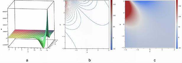
in equation (22), we obtain an exact generalized traveling wave solution to the Fokker–Planck equation. Its graphical representation is shown in figure 7. The solution’s characteristics can be visualized, figure 7(a) displays a three-dimensional surface plot over the spatial-temporal domain $x \in [-2\pi, 2\pi], t \in [-2\pi, 2\pi]$, while the corresponding contour plot and density plot are presented in figures 7(b) and (c), respectively. This solution takes the form $u(x,t) = 2\cos(x + t + 1)e^{x - t + 1} + 3$, exhibiting an oscillatory structure modulated by an exponential factor. The cosine term represents periodic wave-like variations, while the exponential term introduces spatial growth and temporal decay. This behavior reflects the interplay between drift and diffusion in the Fokker–Planck equation.
Figure 7. The generalized traveling wave solution plot of the Fokker–Planck equation.
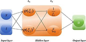
Case 2 The 2-2-2-1 RSENNs model, defined in equation (4), is employed to construct exact solutions of the Fokker–Planck equation, as illustrated in figure 8. By specifying the activation functions as $F_1(\xi_{1}) = \varphi(\xi_{1})$, $F_2(\xi_{2}) = \varphi^2(\xi_{2})$, $F_3(\xi_{3}) = \frac{1}{\xi_{3}}$, and $F_4(\xi_{4}) = \xi_{4}$, where $\varphi(\cdot)$ denotes a solution of the Riccati equation given in equation (2), the Riccati-based function $\varphi(\cdot)$ can generate trigonometric and hyperbolic structures depending on parameter choices; its squared form $\varphi^2(\cdot)$ is used to adjust the amplitude of the solution. The reciprocal function $\frac{1}{(\cdot)}$ introduces rational and singular structures, while the identity mapping $(\cdot)$ preserves linear components.
Figure 8. The 2-2-2-1 RSENNs model of the Fokker–Planck equation.
The trial solution can be written as
$\begin{equation*} u = w_{3,u} \frac{1}{\xi_{3}} + w_{4,u} \xi_{4} + b_5.\end{equation*}$
The trial function $u(x,t)$ is
$\begin{align}u\left(x,t\right)& = \frac{w_{3,u}}{w_{1,3} \varphi \! \left(t w_{t ,1}+x w_{x ,1}+b_{1}\right)+w_{2,3} \varphi \! \left(t w_{t ,2}+x w_{x ,2}+b_{2}\right)^{2}+b_{3}}\\ &\quad +w_{4,u} (w_{1,4} \varphi \! (t w_{t ,1}+x w_{x ,1}+b_{1})+w_{2,4} \varphi \! \left(t w_{t ,2}+x w_{x ,2}+b_{2}\right)^{2}+b_{4})+b_{5}. \end{align}$
We substitute the trial function (24) into equation (19) and simplify the expression, where $\varphi^{^{\prime}} = \sigma + \varphi^2$. By grouping similar terms based on combinations of $t$, $x$, $\varphi \! \left(t w_{t ,1}+x w_{x ,1}+b_{1}\right)$, $\varphi \! \left(t w_{t ,2}+x w_{x ,2}+b_{2}\right)$, then setting the coefficients of each term to zero, we ultimately obtain an undetermined system of nonlinear algebraic equations. This nonlinear system is subsequently solved using the symbolic computation software Maple, twenty-two sets of solutions can be obtained, which are not listed here one by one. The one solution we finally choose is as follows,
$\begin{align} \Big\{\sigma &= \sigma, T_{1} = T_{1}, T_{2} = T_{2}, b_{3} = 0, w_{1,3} = 0,\\ w_{1,4}& = w_{1,4}, w_{2,3} = w_{2,3}, w_{2,4} = w_{2,4},\\ w_{3,u} &= w_{3,u}, w_{4,u} = w_{4,u}, w_{t,1} = -T_{1}w_{x,1},\\ w_{t,2} &= -T_{1}w_{x,2}, w_{x,1} = w_{x,1}, w_{x,2} = w_{x,2}\Big\}. \end{align}$
At this stage, substituting solutions (25) into equation (24) and considering the value of $\sigma$, We can obtain the following exact solutions for the Fokker–Planck equation
$\begin{align} u\left(x,t\right)& = \frac{w_{3,u}}{w_{2,3} \varphi \! \left(-t T_{1} w_{x ,2}+x w_{x ,2}+b_{2}\right)^{2}}\\ &\quad +w_{4,u} \left(w_{1,4} \varphi \! \left(-t T_{1} w_{x ,1}+x w_{x ,1}+b_{1}\right)\right)\\ &\quad +w_{4,u} \left(w_{2,4} \varphi \! \left(-t T_{1} w_{x ,2}+x w_{x ,2}+b_{2}\right)^{2}+b_{4}\right) +b_{5}. \end{align}$
When $\sigma \lt$ 0,
$\begin{align}u_{1}\left(x,t\right) & = -\frac{w_{3,u}}{w_{2,3} \sigma \tanh \! (\sqrt{-\sigma}\,(-t T_{1} w_{x ,2}+x w_{x ,2}+b_{2}))^{2}}\\ &\quad +w_{4,u} (-w_{1,4} \sqrt{-\sigma}\, \tanh \! (\sqrt{-\sigma}\, (-t T_{1} w_{x ,1}\\ &\quad+x w_{x ,1}+b_{1})))\\ &\quad -w_{4,u}(w_{2,4} \sigma (\tanh^{2}(\sqrt{-\sigma}\,\\ &\quad (-t T_{1} w_{x ,2}+x w_{x ,2}+b_{2})))+b_{4})+b_{5}. \end{align}$
$\begin{align} u_{2}\left(x,t\right) = &-\frac{w_{3,u}}{w_{2,3} \sigma \coth \! \left(\sqrt{-\sigma}\, \left(-t T_{1} w_{x ,2}+x w_{x ,2}+b_{2}\right)\right)^{2}}\\ &\quad +w_{4,u} (-w_{1,4} \sqrt{-\sigma}\, \coth \! (\sqrt{-\sigma}\, \\ &\quad (-t T_{1} w_{x ,1}+x w_{x ,1}+b_{1})))\\ & \quad -w_{4,u} (w_{2,4} \sigma (\coth^{2}(\sqrt{-\sigma}\, (-t T_{1} w_{x ,2}+x w_{x ,2}\\ &\quad +b_{2})))+b_{4})+b_{5}. \end{align}$
When $\sigma$ > 0,
$\begin{equation} \begin{aligned} u_{3}(x,t)& = \frac{w_{3,u}}{w_{2,3} \sigma \tan \! (\sqrt{\sigma}\, (-t T_{1} w_{x ,2}+x w_{x ,2}+b_{2}))^{2}}\\ &\quad +w_{4,u} (w_{1,4} \sqrt{\sigma}\, \tan \! (\sqrt{\sigma}\, (-t T_{1} w_{x ,1}+x w_{x ,1}+b_{1})))\\ &\quad +w_{4,u} (w_{2,4} \sigma (\tan^{2}(\sqrt{\sigma}\, (-t T_{1} w_{x ,2}+x w_{x ,2}\\ &\quad +b_{2})))+b_{4})+b_{5}. \end{aligned}\end{equation}$
$\begin{equation} \begin{aligned} u_{4}\left(x,t\right)& = \frac{w_{3,u}}{w_{2,3} \sigma \cot \! \left(\sqrt{\sigma}\, \left(-t T_{1} w_{x ,2}+x w_{x ,2}+b_{2}\right)\right)^{2}}\\ &\quad +w_{4,u} \left(w_{1,4} \sqrt{\sigma}\, \cot \! \left(\sqrt{\sigma}\, \left(-t T_{1} w_{x ,1}+x w_{x ,1}+b_{1}\right)\right)\right)\\ &\quad +w_{4,u} (w_{2,4} \sigma \left(\cot^{2}\left(\sqrt{\sigma}\, \left(-t T_{1} w_{x ,2}+x w_{x ,2}+b_{2}\right)\right)\right)\\ &\quad +b_{4})+b_{5}. \end{aligned}\end{equation}$
When $\sigma$ = 0,
$\begin{align} u_{5}\left(x,t\right)& = \frac{w_{3,u} \left(-t T_{1} w_{x ,2}+x w_{x ,2}+\omega +b_{2}\right)^{2}}{w_{2,3}}\nonumber\\ &\quad -\frac{w_{4,u} w_{1,4}}{-t T_{1} w_{x ,1}+x w_{x ,1}+\omega +b_{1}}\nonumber\\ & \quad +\frac{w_{4,u} w_{2,4}}{\left(-t T_{1} w_{x ,2}+x w_{x ,2}+\omega +b_{2}\right)^{2}}+w_{4,u} b_{4}+b_{5}. \end{align}$
Taking equation (27) as an example, by selecting the coefficients
$\begin{align*} \Big\{w_{4, u} &= 1, w_{3,u} = 2, w_{x,1} = 10, w_{x,2} = 3,\nonumber\\ &\quad w_{t,1} = 2, w_{t,2} = 4, w_{1,3} = 6,\nonumber \\ &\quad w_{1,4} = 7, w_{2,3} = 1, w_{2,4} = 1, b_{1} = 1, T_{1} = 1,\nonumber\\ &\quad b_{2} = 1, b_{5} = 1, b_{3} = 1, b_{4} = 1, T_{2} = 1\Big\}, \end{align*}$
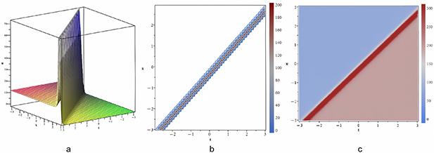
an exact generalized traveling wave solution with singularities to the Fokker–Planck equation is obtained. The graphical representation is shown in figure 9, figure 9(a) displays a three-dimensional surface plot over the spatial-temporal domain $x \in [-\pi, \pi], t \in [-\pi, \pi]$, while figures 9(b) and (c) present the corresponding contour plot and density plot, respectively. This $\tanh$-type solution represents an exact generalized traveling wave with double-kink-like structures, propagating with velocity $c = T_1 = 1$. It exhibits two interacting transition fronts, forming a multi-layer wave profile. The presence of multiple spatial scales reflects the interplay between drift and diffusion in the Fokker–Planck equation, giving rise to complex nonlinear wave dynamics.
Figure 9. The generalized traveling wave solution plot of the Fokker–Planck equation.

4.3. The KdV–mKdV equation

The KdV–mKdV equation is as follows,
$\begin{equation} \frac{\partial u}{\partial t}+ \alpha u\frac{\partial u}{\partial x}+ \beta u^2\frac{\partial u}{\partial x}+ \gamma \frac{\partial^3 u}{\partial x^3} = 0, x\in\left[x_0,x_L\right], t\in\left[0,T\right],\end{equation}$
where $\alpha, \beta,\gamma$ are constants.
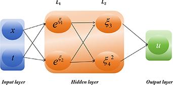
Case 1 The 2-2-2-1 NNAS model, defined in equation (4), is employed to construct exact solutions of the KdV–mKdV equation, as illustrated in figure 10. By specifying the activation functions as $F_1(\xi_{1}) = e^{\xi_{1}}$, $F_2(\xi_{2}) = e^{\xi_{2}}$, $F_3(\xi_{3}) = \xi_{3}$, and $F_4(\xi_{4}) = \xi_{4}^2$, the exponential function $e^{(\cdot)}$ introduces non-periodic growth behavior, the identity mapping $(\cdot)$ preserves linear components, and the squared mapping $(\cdot)^2$ enhances nonlinear effects in the solution.
Figure 10. The 2-2-2-1 NNAS model of the KdV–mKdV equation.
The trial solution can be written as
$\begin{equation*} u = w_{3,u} \xi_{3} + w_{4,u} \xi_{4}^2 + b_5.\end{equation*}$
The trial function $u(x,t)$ is
$\begin{align} u\left(x,t\right)&=w_{4,u} \left(\mathrm{e}^{t w_{t ,1}+x w_{x ,1}+b_{1}} w_{1,4}+\mathrm{e}^{t w_{t ,2}+x w_{x ,2}+b_{2}} w_{2,4}+b_{4}\right)^{2}\\ &\quad +w_{3,u} \left(\mathrm{e}^{t w_{t ,1}+x w_{x ,1}+b_{1}} w_{1,3}+\mathrm{e}^{t w_{t ,2}+x w_{x ,2}+b_{2}} w_{2,3}+b_{3}\right)\\ &\quad+b_{5}. \end{align}$
We substitute the trial function (33) into equation (32) and simplify the expression. By grouping similar terms based on combinations of $t$, $x$, $\mathrm{e}^{t w_{t ,1}+x w_{x ,1}+b_{1}}$, $\mathrm{e}^{t w_{t ,2}+x w_{x ,2}+b_{2}}$ collecting the coefficients of each term and setting them to zero, we obtain an undetermined system of nonlinear algebraic equations. Using software Maple to solve this system of nonlinear algebraic equations, fifty sets of solutions can be obtained, which are not listed here one by one. The one solution we finally choose is as follows,
$\begin{align} \Big\{\alpha &= \alpha, \beta = \beta, b_{3} = b_{3}, b_{4} = b_{4}, b_{5} = -b_{4}^2 w_{4,u} - b_{3}w_{3,u},\\ w_{1,3}& = 0, w_{1,4} = 0, w_{2,3} = 0,\\w_{2,4} &= 0, w_{3,u} = w_{3,u}, w_{4,u} = w_{4,u}, w_{t,1} = w_{t,1}, w_{t,2} = w_{t,2},\\ w_{x,1} &= w_{x,1}, w_{x,2} = w_{x,2}\Big\}.\end{align}$
At this point, substituting (34) into equation (33) yields one form of the exact solutions
$\begin{align} u\left(x,t\right)& = \frac{1}{4 w_{4,u} w_{2,4}^{2}}4 \,\mathrm{e}^{8 \gamma t w_{x ,2}^{3}-2 x w_{x ,2}+2 b_{1}} w_{1,4}^{2} w_{2,4}^{2} w_{4,u}^{2}\\ &\quad +4 \,\mathrm{e}^{-8 \gamma t w_{x ,2}^{3}+2 x w_{x ,2}+2 b_{2}} w_{2,4}^{4} w_{4,u}^{2}\\ &\quad +8 w_{4,u}^{2} w_{2,4}^{3} w_{1,4} \mathrm{e}^{b_{1}+b_{2}}+4 w_{4,u} \left(b_{3} w_{3,u}+b_{5}\right) w_{2,4}^{2}\\ & \quad +w_{2,3}^{2} w_{3,u}^{2} w_{2,4}^{2}. \end{align}$
By selecting the coefficients
$\begin{align*} \Big\{w_{4, u} &= 1, w_{3,u} = 2, w_{x,1} = 1, w_{x,2} = 2, w_{t,1} = 2,\\ w_{t,2} &= 4, w_{1,3} = 6, w_{1,4} = 7,\\ w_{2,3}& = 1, w_{2,4} = 1, b_{1} = 1, b_{2} = 1, b_{5} = 1,\\ b_{3}& = 1, b_{4} = 1, \alpha = 1, \gamma = 1 \Big\},\end{align*}$
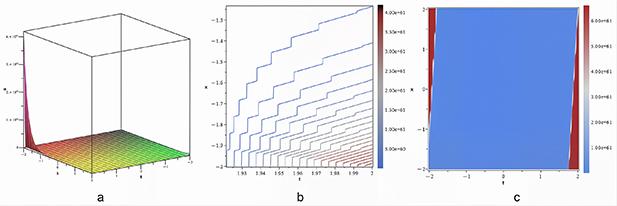
in equation (35), we obtain an exact exponential-type asymmetric traveling wave solution to the KdV–mKdV equation. Its graphical representation shown in figure 11, figure 11(a) presents a three-dimensional surface plot over the spatial-temporal domain $x \in [-2, 2], t \in [-2, 2]$, while figures 11(b) and (c) display the corresponding contour plot and density plot, respectively. This solution represents a traveling wave propagating with velocity $c = 16$, exhibiting an asymmetric structure formed by exponential components. The imbalance between these components leads to a non-uniform spatial profile. This behavior reflects the interplay between nonlinearity and dispersion in the KdV–mKdV equation.
Figure 11. The exponential-type asymmetric traveling wave solution plot of the KdV–mKdV equation.
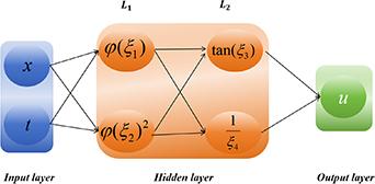
Case 2 The 2-2-2-1 RSENNs model, defined in equation (4), is employed to construct exact solutions of the KdV–mKdV equation, as illustrated in figure 12. By specifying the activation functions as $F_1(\xi_{1}) = \varphi(\xi_{1})$, $F_2(\xi_{2}) = \varphi^2(\xi_{2})$, $F_3(\xi_{3}) = \tan(\xi_{3})$, and $F_4(\xi_{4}) = \frac{1}{\xi_{4}}$, where $\varphi(\cdot)$ denotes a solution of the Riccati equation given in equation (2), the Riccati-based function $\varphi(\cdot)$ can generate trigonometric and hyperbolic structures depending on parameter choices; its squared form $\varphi^2(\cdot)$ enhances nonlinear effects in the solution. The tangent function $\tan(\cdot)$ introduces periodic structures, while the reciprocal function $\frac{1}{(\cdot)}$ introduces rational and singular structures.
Figure 12. The 2-2-2-1 RSENNs model of the KdV–mKdV equation.
The trial solution can be written as
$\begin{equation*} u = w_{3,u} \tan\left(\xi_{3}\right) + w_{4,u} \frac{1}{\xi_{4}} + b_5.\end{equation*}$
The trial function $u(x,t)$ is
$\begin{align} u\left(x,t\right)& = w_{3,u} \tan \! \left(w_{1,3} \varphi \! \left(t w_{t ,1}+x w_{x ,1}+b_{1}\right)+w_{2,3} \varphi \! \left(t w_{t ,2}+x w_{x ,2}+b_{2}\right)^{2}+b_{3}\right)\nonumber\\ &\quad+\frac{w_{4,u}}{w_{1,4} \varphi \! \left(t w_{t ,1}+x w_{x ,1}+b_{1}\right)+w_{2,4} \varphi \! \left(t w_{t ,2}+x w_{x ,2}+b_{2}\right)^{2}+b_{4}}+b_{5}. \end{align}$
We substitute the trial function (36) into equation (32) and simplify the expression, where $\varphi^{^{\prime}} = \sigma + \varphi^2$. By grouping similar terms based on combinations of $t$, $x$, $\varphi \! \left(t w_{t ,1}+x w_{x ,1}+b_{1}\right)$, $\varphi \! \left(t w_{t ,2}+x w_{x ,2}+b_{2}\right)$, $\tan \! (w_{1,3} \varphi \! \left(t w_{t ,1}+x w_{x ,1}+b_{1}\right)+w_{2,3} \varphi \! \left(t w_{t ,2}+x w_{x ,2}+b_{2}\right)^{2}+b_{3})$, then setting the coefficients of each term to zero, we ultimately obtain an undetermined system of nonlinear algebraic equations.This nonlinear system is subsequently solved using the symbolic computation software Maple, twenty-one sets of solutions can be obtained, which are not listed here one by one. The one solution we finally choose is as follows,
$\begin{align} \{\alpha &= \alpha, \beta = \beta, \sigma = 0, b_{4} = b_{4}, b_{5} \\ &= -\frac{2\alpha b_{4} + 3\beta w_{4,u}}{4b_{4}\beta}, w_{1,3} = w_{1,3}, w_{1,4} = 0,\\ w_{2,3} & = w_{2,3}, w_{2,4} = \frac{24\gamma b_{4}^3 w_{x,2}^2}{\beta w_{4,u}^2}, w_{3,u} = 0,\\ w_{4,u} & = w_{4,u}, w_{t,1} = w_{t,1},\\ w_{t,2} & = \frac{w_{x,2}\left(4\alpha^2b_{4}^2 - \beta^2 w_{4,u}^2\right)}{16b_{4}^2\beta},\\ w_{x,1} & = w_{x,1}, w_{x,2} = w_{x,2}\Big\}. \end{align}$
At this stage, by substituting the coefficient solutions (37) into equation (36) and considering the value of $\sigma$, we can obtain the following exact solution for the KdV–mKdV equation
$\begin{align} u\left(x,t\right) & = \frac{w_{4,u}}{\frac{24 \gamma b_{4}^{3} w_{x ,2}^{2} {\varphi \left(\frac{t w_{x ,2} \left(4 \alpha^{2} b_{4}^{2}-\beta^{2} w_{4,u}^{2}\right)}{16 b_{4}^{2} \beta}+x w_{x ,2}+b_{2}\right)}^{2}}{\beta w_{4,u}^{2}}+b_{4}}\\ &\quad-\frac{2 \alpha b_{4}+3 \beta w_{4,u}}{4 b_{4} \beta}. \end{align}$
Considering the case of $\sigma = 0$ based on equation (2),
$\begin{align} u\left(x,t\right) & = \frac{w_{4,u}}{\frac{24 \gamma b_{4}^{3} w_{x ,2}^{2}}{\beta w_{4,u}^{2} {\left(\frac{t w_{x ,2} \left(4 \alpha^{2} b_{4}^{2}-\beta^{2} w_{4,u}^{2}\right)}{16 b_{4}^{2} \beta}+x w_{x ,2}+b_{2}+\omega \right)}^{2}}+b_{4}}\\ &\quad-\frac{2 \alpha b_{4}+3 \beta w_{4,u}}{4 b_{4} \beta}.\end{align}$
By selecting the coefficients
$\begin{align*} \Big\{w_{4,u} &= 3,b_{1} = 1,T_{1} = 1,w_{x,2} = 2,b_{2} = 1,w_{2,4} = 1,\\ w_{1,4}& = 6,b_{5} = 1,\alpha = 1,b_{4} = 1,\\ T_{2} &= 1,b_{3} = 1,\sigma = -2,w_{x,1} = 1,w_{3,u} = 1,w_{1,3} = 1,\\ w_{2,3}& = 1,\beta = 2,\gamma = 5,\omega = 3\Big\}, \end{align*}$
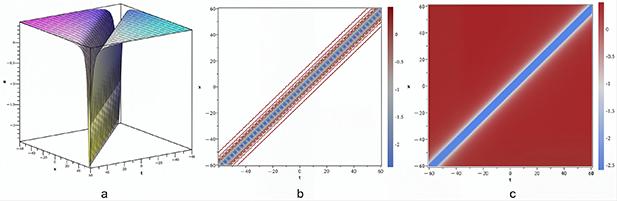
this gives an exact generalized soliton-type solution to the KdV–mKdV equation. The graphical representation is shown in figure 13, figure 13(a) displays a three-dimensional surface over the spatio-temporal domain [$-$50, 50]$\times$[$-$60, 60], while the corresponding contour plot and density plot are presented in figures 13(b) and (c), respectively. This solution represents a generalized algebraic dark soliton traveling with velocity $c = 1$, exhibiting a localized dip structure. It illustrates the balance between nonlinear steepening and dispersive spreading in the KdV–mKdV equation, giving rise to a stable, localized wave profile.
Figure 13. The generalized soliton-type solution plot of the KdV–mKdV equation.

5. Discussions

To evaluate the advantages of the RSENNs method over the NNAS method, this section provides a comparison and analysis of the solutions to the Burgers equation.
The two sets of solutions obtained using the NNAS method for the Burgers equation,
$\begin{align}u_{1}\left(x,t\right) & = 2 \tan \! \left(\left(-t b_{5} w_{x ,1}+x w_{x ,1}+b_{1}\right) w_{1,4}+b_{4}\right) \nonumber\\ &\qquad \alpha w_{1,4} w_{x ,1}+b_{5}. \end{align}$
$\begin{align} u_{2}\left(x,t\right) & = -2 \cot \! \left(\left(-t b_{5} w_{x ,1}+x w_{x ,1}+b_{1}\right) w_{1,3}+b_{3}\right) \nonumber\\ &\qquad \alpha w_{1,3} w_{x ,1}+b_{5}. \end{align}$
The five sets of solutions obtained using the RSENNs method for the Burgers equation,
$\begin{align} u_{3}\left(x,t\right) = b_{3} w_{3,u}-\frac{2 \alpha w_{x ,1} \left(\sigma w_{1,4}^{2}+b_{4}^{2}\right)}{w_{1,4} \left(w_{1,4} \sqrt{\sigma}\, \tan \! \left(\sqrt{\sigma}\, \xi_{1}\right)+b_{4}\right)}+b_{5}, \end{align}$
$\begin{align} u_{4}\left(x,t\right) = b_{3} w_{3,u}-\frac{2 \alpha w_{x ,1} \left(\sigma w_{1,4}^{2}+b_{4}^{2}\right)}{w_{1,4} \left(-w_{1,4} \sqrt{\sigma}\, \cot \! \left(\sqrt{\sigma}\, \xi_{1}\right)+b_{4}\right)}+b_{5},\end{align}$
where $\alpha$ is a constant, $\xi_{1} = \frac{t w_{x ,1} \left(2 \alpha b_{4} w_{x ,1}-b_{3} w_{1,4} w_{3,u}-b_{5} w_{1,4}\right)}{w_{1,4}}+x w_{x ,1}+b_{1}$.
$\begin{align} u_{5}\left(x,t\right) & = b_{3} w_{3,u}\nonumber\\ &\quad -\frac{2 \alpha w_{x ,1} \left(\sigma w_{1,4}^{2}+b_{4}^{2}\right)}{w_{1,4} \left(-w_{1,4} \sqrt{-\sigma}\, \tanh \! \left(\sqrt{-\sigma}\, \xi_{1} \right)+b_{4}\right)}+b_{5}, \end{align}$
$\begin{align}u_{6}\left(x,t\right)& = b_{3} w_{3,u}\nonumber\\ &\quad -\frac{2 \alpha w_{x ,1} \left(\sigma w_{1,4}^{2}+b_{4}^{2}\right)}{w_{1,4} \left(-w_{1,4} \sqrt{-\sigma}\, \coth \! \left(\sqrt{-\sigma}\, \xi_{1} \right)+b_{4}\right)}+b_{5}, \end{align}$
where $\alpha$ is a constant, $\xi_{1} = \frac{t w_{x ,1} \left(2 \alpha b_{4} w_{x ,1}-b_{3} w_{1,4} w_{3,u}-b_{5} w_{1,4}\right)}{w_{1,4}}+x w_{x ,1}+b_{1}$.
$\begin{align} u_{7}\left(x,t\right) = b_{3} w_{3,u}-\frac{2 \alpha w_{x ,1} \left(\sigma w_{1,4}^{2}+b_{4}^{2}\right)}{w_{1,4} \left(-\frac{w_{1,4}}{\xi_{1}+\omega}+b_{4}\right)}+b_{5}, \end{align}$
where $\omega$ and $\alpha$ are a constants, $\xi_{1} = \frac{t w_{x ,1} \left(2 \alpha b_{4} w_{x ,1}-b_{3} w_{1,4} w_{3,u}-b_{5} w_{1,4}\right)}{w_{1,4}}+x w_{x ,1}+b_{1}$.
Analysis of the above solutions, when $-b_{5}w_{x,1}w_{1,4} = \sqrt{\sigma}w_{x,1}\frac{2\alpha b_{4}w_{x,1}-b_{3}w_{1,4}w_{3,u}-b_{5}w_{1,4}}{w_{1,4}}$, $w_{x,1}w_{1,4} = \sqrt{\sigma}w_{x,1}$, $b_{4} = 0$, $w_{1,4}b_{1} = \sqrt{\sigma}b_{1}$, $-\frac{2\alpha w_{x,1}(\sigma w_{1,4}^2+b_{4}^2)}{-w_{1,4}^2 \sqrt{\sigma}} = 2\alpha w_{1,4}w_{x,1}$, $u_{1}(x,t)$ and $u_{4}(x,t)$ have the same exact solution. Similarly, after determining some of the coefficients, $ u_2 (x,t)$ and $ u_3 (x,t)$ should have the same exact solution.
The preceding section has demonstrated, using the Burgers equation as an example, that the RSENNs method can reproduce the solutions of the NNAS method. Table 1 presents a quantitative comparison of the three equations: for the Burgers equation, the RSENNs method generates 28 equations (1.18 s) with 30 coefficient solutions, while the NNAS method generates 135 equations (2.46 s) with 30 coefficient solutions; for the Fokker–Planck equation, the RSENNs method produces 39 equations (1.46 s) with 22 coefficient solutions, compared to 8 from the NNAS method; for the KdV–mKdV equation, the RSENNs method produces 492 equations (2.96 s) with 21 coefficient solutions, compared to 50 from the NNAS method.
Table 1. Quantitative comparison between NNAS and RSENNs methods.
NNAS RSENNs
Equation Equations Time (s) Coeff. Equations Time (s) Coeff.
Burgers 135 2.46 30 28 1.18 30
Fokker–Planck 2 0.45 8 39 1.46 22
KdV–mKdV 15 0.96 50 492 2.96 21

Bold values indicate relatively better performance in terms of smaller system size, shorter computation time, or larger number of coefficient solutions. Time refers to Maple symbolic solving only, excluding activation function design. ‘Coeff.’ denotes the number of coefficient solutions.

The above results indicate that the core advantage of the RSENNs method does not lie in consistently reducing symbolic computation costs or in obtaining more solutions in all cases, but rather in improving the efficiency at the preprocessing stage and providing a more systematic way to generate diverse solution structures. By employing the Riccati solutions family as a unified activation function library, the RSENNs method reduces the time required for activation function design compared with the NNAS method. For the Fokker–Planck equation, the RSENNs method obtains more coefficient solutions than the NNAS method (22 vs 8), indicating its capability to enrich the diversity of solution forms under certain configurations. However, for the KdV–mKdV equation, the RSENNs method yields fewer coefficient solutions (21 vs 50), suggesting that the performance of the method depends on the specific equation and the selected network structure.
However, the RSENNs method also has several limitations. First, restricted solution forms, the obtained solutions are mainly limited to hyperbolic functions, trigonometric functions, rational functions, and their combinations, and may not adequately represent other types such as exponential or algebraic functions. Second, architecture design relies on experience, there is a lack of systematic criteria for selecting the number of hidden layers and neurons, and the performance of the method depends on the specific equation structure, as reflected by the varying results across the three equations (comparable for the Burgers equation, higher for the Fokker–Planck equation, and lower for the KdV–mKdV equation in terms of coefficient solution count). Third, scalability bottleneck, high-dimensional problems lead to rapid growth in the size of algebraic equation systems, and with the increase in networks complexity, the computational difficulty also increases. Finally, regarding the relationship to existing work, Mohammad et al proposed the basic framework of the RSENNs method. In this paper, we introduce a form-selection strategy ($\varphi$, $\varphi^2$, $\frac{1}{\varphi}$) and apply it systematically to three types of equations, which can be viewed as an extension and further development of the existing method. This also implies that form selection currently relies on prior knowledge of equation structures and lacks automated selection criteria, which may lead to suboptimal networks configurations for certain equations.

6. Conclusions

In recent years, with the rapid development of deep learning techniques, neural networks methods have demonstrated great potential in various fields, including physics, biology, and engineering. By integrating traditional mathematical methods with neural networks, researchers have gradually explored and refined new paradigms for solving PDEs.
This paper is based on the RSENNs method proposed by Mohammad et al which uses solutions of the Riccati equation as activation functions, and further introduces a form selection strategy to extend the Riccati solution from a single form to multiple forms. The proposed method is systematically applied to the Burgers equation, the Fokker–Planck equation, and the KdV–mKdV equation. By comparison with the NNAS method, the effectiveness of the RSENNs method is validated, particularly in improving efficiency at the preprocessing stage.
In the NNAS method, an explicit neural networks model is constructed as the trial function for PDEs solutions. The trial function is substituted into the target equation, and the coefficients of the resulting expressions are set to zero, leading to a system of nonlinear algebraic equations. This system is then solved using symbolic computation software (e.g. Maple), and the obtained coefficients are substituted back into the trial function to derive exact solutions of the PDEs. However, the NNAS method requires designing specific activation functions for each problem, lacks general construction rules, and may limit the diversity of obtainable solutions.
The core feature of the RSENNs method lies in using different solutions forms of the Riccati equation as activation functions within the neural networks architecture. By utilizing the Riccati equation solutions family as a unified activation function library, the method reduces the lengthy and complex derivation process required for activation function design. Furthermore, the form selection strategy enables a more systematic generation of activation functions. To illustrate the dynamic characteristics of the solutions, various visualizations are generated using software Maple, including three-dimensional plots, contour plots, and density plots. Comparative analysis with the NNAS method shows that the RSENNs method improves efficiency in the preprocessing stage and provides more diverse solution structures.
Future research can explore several directions to address the limitations identified in this study. To overcome the restriction of solutions forms, future work may focus on constructing more general activation functions libraries by incorporating exponential, algebraic, and elliptic functions beyond the Riccati solutions family, thereby enhancing the expressiveness of the solution space. To reduce reliance on empirical architecture design, it is important to develop systematic and theoretically grounded criteria for determining the number of hidden layers and neurons, thereby improving reproducibility. As an intermediate approach, integrating neural networks frameworks with symbolic computation or evolutionary algorithms may enable semi-automated architecture design. To address scalability issues in high-dimensional problems, dimensionality reduction techniques and parallel computing strategies may help mitigate the rapid growth of algebraic systems. To reduce dependence on prior knowledge in form selection, future work may explore automated selection strategies based on equation structure analysis or data-driven approaches. Furthermore, integrating the current framework with advanced architectures such as Residual networks [35] and KAN networks [36, 37] may improve representation capability and enhance the ability to handle more complex problems.

We appreciated the support by the Natural Science Foundation of Shandong Province (No. ZR2023MA062), National Natural Science Foundation of China (No. 42502224), Fundamental Research Program of Shanxi Province (No. 202403021222001), the Belt and Road Special Foundation of the State Key Laboratory of Water Disaster Prevention (2023491911).

1
Polyanin A D 2025 Principle of structural analogy of solutions and its application to nonlinear PDEs and delay PDEs J. Math. Sci. 289 487 497

DOI

2
Wazwaz A M 2009 Partial Differential Equations and Solitary Waves Theory Springer

3
Rathinasamy S, Chun C B, Bae AR 2010 A general approach to hyperbolic partial differential equations by homotopy perturbation method Int. J. Comput. Math. 87 2601 2606

DOI

4
Ancona F, Bianchini S 2025 Preface: recent advances in nonlinear hyperbolic PDEs and fluid dynamics J. Hyperbolic Differ. Equ. 21 501 502

DOI

5
Zhukovsky K, Oskolkov D 2020 Modeling of heat transport and exact analytical solutions in thin films with account for constant non-relativistic motion Int. J. Heat Mass Transfer. 150 119085 119085

DOI

6
Wang R 2018 Symmetry transformations and exact solutions of a generalized hyperelastic rod equation CMC-Comput. Mater. Con. 55 345 357

DOI

7
Lv N, Li J, Yuan X, Wang R 2023 Controllable rogue waves in a compressible hyperelastic plate Phys. Lett. A 461 128639

DOI

8
Seadawy A R 2017 Solitary wave solutions of two-dimensional nonlinear Kadomtsev-Petviashvili dynamic equation in dust-acoustic plasmas Pramana-J. Phys. 89 485

DOI

9
Islam S M R, Khan S, Arafat S M Y, Akbar M A 2022 Diverse analytical wave solutions of plasma physics and water wave equations Results Phys. 40 105834

DOI

10
Kumar S, Mohan B, Kumar R 2022 Lump, soliton and interaction solutions to a generalized two-mode higher-order nonlinear evolution equation in plasma physics Nonlinear Dyn. 110 693 704

DOI

11
Kumar S, Mohan B, Kumar A 2022 Generalized fifth-order nonlinear evolution equation for the Sawada Kotera, Lax and Caudrey-Dodd-Gibbon equations in plasma physics: Painleve’ analysis and multi-soliton solutions Phys. Scr. 97 035201

DOI

12
Alkhazaleh O, Nergard J, Shepherd C 2025 Exact solutions for real and complex nonlinear partial differential equations in engineering using a modified homotopy perturbation method Eng. Sci. 36 1573

DOI

13
Liu Y 2025 Modified homotopy perturbation methods for solving partial differential equations J. Appl. Anal. Comput. 15 2853 2865

DOI

14
Khan U A M 2024 Soliton solutions of nonlinear coupled Davey-Stewartson Fokas system using modified auxiliary equation method and extended ($\frac{G^{^{\prime}}}{G^2}$) -expansion method Sci. Rep. 14 21949

DOI

15
Pleumpreedaporn C, Moore E J, Sirisubtawee S, Khansai N, Pleumpreedaporn S 2024 Exact solutions for the Sharma-Tasso-Olver equation via the Sardar subequation method with a comparison between Atangana Space-Time beta-derivatives and classical derivatives Mathematics 12 2155 2155

DOI

16
Ali A R 2025 Precise soliton solutions of the Landau-Ginzburg-Higgs equation via the Sardar sub-equation method Discov. Appl. Sci. 7 1 17

DOI

17
Zhao C Y, Wu J, Yang Z 2026 An extended $\frac{G^{^{\prime}}}{G}$-expansion method for the conformable space-time fractional Newell-Whitehead-Segel equation: Exact traveling-wave solutions and regularity features AIMS Math. 11 11347 11371

DOI

18
Hossain A K M K S H, Akter H, Akbar M A 2024 Soliton solutions of DSW and Burgers equations by generalized $\frac{G^{^{\prime}}}{G}$-expansion method Opt. Quantum Electron. 56 1 24

DOI

19
Zhang R F, Li M C, Cherraf A, Vadyala S R 2023 The interference wave and the bright and dark soliton for two integro-differential equation by using BNNM Nonlinear Dyn. 111 8637 8646

DOI

20
Zhang R F, Li M-C, Gan J-Y, Li Q, Lan Z-Z 2022 Novel trial functions and rogue waves of generalized breaking soliton equation via bilinear neural network method Chaos Solitons Fractals 154 111692

DOI

21
Qasim M, Yao F, Baber M Z 2025 Explicit wave solutions profile of (3+1)-dimensional Bateman-Burgers equation via bilinear neural network method Eur. Phys. J. Plus 140 224

DOI

22
Nguyen M T, Meesad P 2025 Bilinear recurrent neural network for a modified Benney-Luke equation Int. J. Appl. Comput. Math. 11 35

DOI

23
Liu Y Q 2025 A novel ($\frac{G^{^{\prime}}}{G}$)-expansion neural networks method for exactly explicit solutions of nonlinear partial differential equations Nonlinear Dyn. 113 26603 26630

DOI

24
Zhang Y, Zhang R F, Yuen K V 2023 Neural network-based analytical solver for Fokker-Planck equation Eng. Appl. Artif. Intell. 125 106721

DOI

25
Muhammad J, Tipu G H, Alrashedi Y, Alrashedi Y 2025 Analytical study of the nonlinear dynamical systems: application of the neural networks method AIMS Math. 10 14596 15116

DOI

26
Muhammad J, Abdullah A R, Yao F P, Younas U 2025 Dynamics of soliton solutions to nonlinear dynamical equations in mathematical physics: application of neural network-based symbolic methods Mathematics 13 3546 3546

DOI

27
Li M, Muhammad J, Yaro D, Tipu G H, Younas U 2025 Investigation of the exact solutions via sub-equation neural network method to the nonlinear systems in fluid and nuclear physics AIP Adv. 15 075208

DOI

28
Muhammad J, Tedjani A H, Hussain E, Younas U 2025 Exploring the exact solutions to the nonlinear systems with neural networks method Sci. Rep. 15 36818

DOI

29
Zhang S, Zhang H Q 2011 Fractional sub-equation method and its applications to nonlinear fractional PDEs Phys. Lett. A. 375 1069 1073

DOI

30
Maaoui W, Mehrez Z, Najjari M 2025 A comparison between artificial neural network and random forest on predicting ferrofluids viscosity under magnetic field application Acta Mech. Sin. 41 724944

DOI

31
Wang J W 2025 Fractional sub-equation neural networks (fSENNs) method for exact solutions of space-time fractional partial differential equations Chaos 35 043110

DOI

32
Wan Q Z 2025 High-dimensional memristor-coupled multiple neural networks with spatial multi-structure attractors and application in image encryption Chaos Solitons Fractals 199 116716

DOI

33
Wang J, Yau S S T, Huang J 2000 Approximate nonlinear output regulation based on the universal approximation theorem Int. J. Robust Nonlinear Control. 10 439 456

DOI

34
Hornik K, Stinchcombe M, White H 1989 Multilayer feedforward networks are universal approximators Neural Netw. 2 359 366

DOI

35
Ma Z M, Liu Y L, Wang Y L 2024 The exact analytical solutions of the (2+1)-dimensional extended Korteweg-de Vries equation using bilinear neural network method and bilinear residual network method Mod. Phys. Lett. B 39 2550045

DOI

36
Yatin K, Vats R K 2026 A deep Kolmogorov–Arnold Network framework for solving time–fractional partial differential equations Appl. Soft Comput. 188 114379

DOI

37
Anjum M W 2025 Application of Kolmogorov-Arnold network (KAN) for solitary-Peakon investigation of Lax model Case Stud Therm. Eng. 73 106537

DOI

Outlines

/