

1. Introduction
2. Model description
2.1. Traveling wave transformation, translation processing, and hard constraints
| • Current-time component $u_0$: The input to the shared neural network is the concatenated feature of all $M$ traveling wave invariants at the current point $(n,t)$: $\begin{align} u_0 = \mathcal{N}\left( \left[ \xi_1\left(n,t\right), \xi_2\left(n,t\right), \dots, \xi_M\left(n,t\right) \right] \right),\end{align}$ where $\mathcal{N}(\cdot)$ represents the shared fully connected neural network with tanh activation and Xavier initialization. | |
| • Translated components $\{u_1, u_2, \dots, u_M\}$: For the $m$-th soliton, we calculate the translated spacetime point at the previous time step $t-\Delta t$, where $\Delta t$ denotes the fixed time step for hard constraint and is set to a constant value of $0.01$ in all experiments: $\begin{align} \left(n_m^{^{\prime}}, t^{^{\prime}}\right) = \left( n - v_m \cdot \Delta t, \, t - \Delta t \right).\end{align}$ The input to the shared neural network for $u_m$ is the concatenated feature of all $M$ traveling wave invariants at this translated point: $\begin{align} u_m = \mathcal{N}\left( \left[ \xi_1\left(n_m^{^{\prime}}, t^{^{\prime}}\right), \xi_2\left(n_m^{^{\prime}}, t^{^{\prime}}\right), \dots, \xi_M\left(n_m^{^{\prime}}, t^{^{\prime}}\right) \right] \right).\end{align}$ | |
| • Unified hard constraint fusion: The final prediction of the wave field $u(n,t)$ is obtained by fusing all components to enforce time-step consistency and translational invariance: $\begin{align} u_{\text{pred}}\left(n,t\right) = \frac{u_0 + \sum_{m = 1}^M u_m}{2}.\end{align}$ |
2.2. Neural network architecture
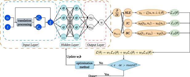
Figure 1. Schematic of the TC-PINNs network architecture based on discrete NLEs. |
2.3. Data preparation and training, network configuration, and model evaluation
2.4. Summary of the TC-PINNs method
| • A traveling wave transformation reduces the discrete NLEs’ spacetime variables $n, t$ to a single variable $\xi = n - vt$, applicable to constant-speed solitons. | |
| • Solitons propagate at a constant speed while preserving their properties. By enforcing neural network outputs to be consistent under spatial translation, the translational invariance is naturally satisfied. |
Table 1. Summary of the TC-PINNs framework (Discrete mKdV equation). |
| Step | Implementation details |
|---|---|
| Step 1 | Traveling wave transformation and translation processing |
| • Traveling-wave transformations: Construct $M$ traveling wave invariants $\xi_m = n - v_m t$, $m = 1,2,\dots,M$ | |
| where $v_m$ is the exact physical velocity of the $m$-th soliton (fixed analytical values) | |
| • Translation-invariant coordinates at previous time step $t-\Delta t$: | |
| For the $m$-th soliton, translated point $(n_m^{^{\prime}}, t^{^{\prime}}) = (n - v_m \cdot \Delta t, t - \Delta t)$ | |
| where $\Delta t = 0.01$ is the fixed time step for hard constraint | |
| • Multi-basis implementation: Concatenate all $M$ traveling wave invariants into a feature vector: | |
| For current time: $\left[\xi_1(n,t), \xi_2(n,t), \dots, \xi_M(n,t)\right]$ | |
| For translated point: $\left[\xi_1(n_m^{^{\prime}}, t^{^{\prime}}), \dots, \xi_M(n_m^{^{\prime}}, t^{^{\prime}})\right]$ | |
| • Neural network mapping: Shared fully connected network $\mathcal{N}(\cdot)$ (tanh activation, Xavier initialization) | |
| Current-time component: $u_0 = \mathcal{N}\left(\left[\xi_1(n,t), \dots, \xi_M(n,t)\right]\right)$ | |
| Translated components: $u_m = \mathcal{N}\left(\left[\xi_1(n_m^{^{\prime}}, t^{^{\prime}}), \dots, \xi_M(n_m^{^{\prime}}, t^{^{\prime}})\right]\right)$, $m = 1,\dots,M$ | |
| • Hard constraint output fusion: | |
| Final prediction: $u_{\text{pred}}(n,t) = \frac{u_0 + \sum_{m = 1}^M u_m}{2}$ | |
| | |
| Step 2 | Neural network architecture |
| • Input layer: Process 2D spatiotemporal data | |
| • Hidden layers: | |
| – 4 hidden layers in total | |
| – Number of neurons per layer: 32/64 (32 for one-soliton/first-order rational soliton (RS), 64 for two-soliton) | |
| • Activation function: Hyperbolic tangent (tanh) | |
| • Residual computation: | |
| – Automatic differentiation on the time dimension of the discrete mKdV equation | |
| – Forward and backward difference on spatial dimension ($n \pm i$ to represent $u_{n\pm i}$) | |
| – Residual expression: $\xi(u, n \pm i, \theta)$ | |
| | |
| Step 3 | Loss function formulation |
| • Total loss: $\mathcal{L}(\theta) = w_1\mathcal{L}_\mathrm{F}(\theta) + w_2\mathcal{L}_\mathrm{I}(\theta) + w_3\mathcal{L}_\mathrm{B}(\theta) + w_4\mathcal{L}_\mathrm{S}(\theta) + w_5\mathcal{L}_\mathrm{T}(\theta)$ | |
| • Component details: | |
| – $\mathcal{L}_\mathrm{F}(\theta) = \frac{1}{N_\mathrm{F}} \sum_{i = 1}^{N_\mathrm{F}} \left| u_t - \xi(u, n \pm i; \theta) \right|^2$: Physics equation loss | |
| – $\mathcal{L}_\mathrm{I}(\theta) = \frac{1}{N_\mathrm{I}} \sum_{j = 1}^{N_\mathrm{I}} \left| u_\theta(t_0, n_i) - u_0(n_i) \right|^2$: Initial condition loss | |
| – $\mathcal{L}_\mathrm{B}(\theta) = \frac{1}{N_\mathrm{B}} \sum_{k = 1}^{N_\mathrm{B}} \left| u_\theta(t_i, n_{\mathrm{B},i}) - u_\mathrm{B}(t_i) \right|^2$: Boundary condition loss | |
| – $\mathcal{L}_\mathrm{S}(\theta) = \frac{1}{N_\mathrm{S}} \sum_{m = 1}^{N_\mathrm{S}} \left| u_\theta(t_i, n_i) - u_\theta(2c_t - t_i, 2c_n - n_i) \right|^2$: Symmetry loss | |
| – $\mathcal{L}_\mathrm{T}(\theta) = \frac{1}{N_\mathrm{T}} \sum_{n = 1}^{N_\mathrm{T}} \left| u_0 - \frac{u_0 + \sum_{m = 1}^M u_m}{2} \right|^2$: Translation symmetry loss | |
| – Different weights $w_i$ assigned to each loss term for correct physical law learning | |
| | |
| Step 4 | Training Strategy and Configuration |
| • Optimization: Two-phase training | |
| – Pre-training: Adam optimizer (learning rate = $1 \times 10^{-3}$) | |
| – Fine-tuning: L-BFGS optimizer (learning rate = $1.0$) | |
| • Data sampling: Hammersley sampling method to generate training set $N_\mathrm{F}$ | |
| • Evaluation metrics: | |
| – Overall Relative Error (RE): $\text{RE} = \frac{\|u_{\theta,k} - u_{\text{true},k}\|_2}{\|u_{\text{true},k}\|_2}$ | |
| – $\text{RE}_{\text{Ins}}$: Inside predicting relative error | |
| – $\text{RE}_{\text{Ext}}$: Extrapolation relative error | |
| • Runtime environment: | |
| – Python 3.11.7, PyTorch 2.7.0+cu126 | |
| – High-performance computer with NVIDIA GeForce RTX 4060 laptop GPU | |
3. Data-driven solutions of equation (1 )
3.1. Numerical simulation of one-soliton solution to equation (1 )
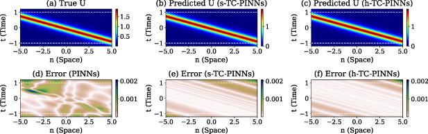
Figure 2. Data-driven one-soliton solution for equation ( |
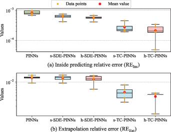
Figure 3. Boxplots of inside predicting and extrapolation relative errors for one-soliton solution with different methods (PINNs, s-SDE-PINNs, h-SDE-PINNs, s-TC-PINNs, h-TC-PINNs) using 5 random seeds per model. |
Table 2. Accuracy and time consumption of numerical simulation for one-soliton solution under different models. Values in bold represent inside predicting and extrapolation relative errors of models with hard constraints, and the training time of h-TC-PINNs is also marked in bold, so as to intuitively compare whether our method achieves superior computational efficiency. |
| Model | $\text{RE}_{\text{Ins}}$ | $\text{RE}_{\text{Ext}}$ | Time |
|---|---|---|---|
| PINNs | $(8.32 \pm 1.13) \times 10^{-4}$ | $(1.32 \pm 0.21) \times 10^{-2}$ | $(111.73\pm15.31)$s |
| s-SDE-PINNs | $(6.14 \pm 1.14) \times 10^{-4}$ | $(1.31 \pm 0.23) \times 10^{-2}$ | $(112.11\pm8.29)$s |
| h-SDE-PINNs | $\mathbf{(5.58 \pm 0.86) \times 10^{-4}}$ | $\mathbf{(1.20 \pm 0.33) \times 10^{-2}}$ | $(91.97\pm12.65)$s |
| s-TC-PINNs | $(2.75 \pm 0.95) \times 10^{-4}$ | $(5.05 \pm 1.99) \times 10^{-3}$ | $(77.12\pm12.22)s$ |
| h-TC-PINNs | $\mathbf{(2.11 \pm 0.95) \times 10^{-4}}$ | $\mathbf{(4.01 \pm 1.36) \times 10^{-3}}$ | $\mathbf{(68.01\pm2.59)\mathrm{s}}$ |
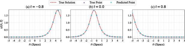
Figure 4. The time evolution of one-soliton solution at three different space-time points based on h-TC-PINNs. |
3.2. Numerical simulation of two-soliton solution to equation (1 )
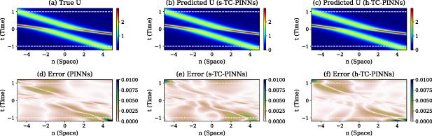
Figure 5. Data-driven two-soliton solution for equation ( |
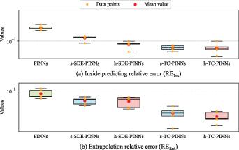
Figure 6. Boxplots of inside predicting and extrapolation relative errors for two-soliton solution with different methods (PINNs, s-SDE-PINNs, h-SDE-PINNs, s-TC-PINNs, h-TC-PINNs) using five random seeds per model. |
Table 3. Accuracy and time consumption of numerical simulation for two-soliton solution under different models. Values in bold represent inside predicting and extrapolation relative errors of models with hard constraints, and the training time of h-TC-PINNs is also marked in bold, so as to intuitively compare whether our method achieves superior computational efficiency. |
| Model | $\text{RE}_{\text{Ins}}$ | $\text{RE}_{\text{Ext}}$ | Time |
|---|---|---|---|
| PINNs | $(1.42 \pm 0.28) \times 10^{-3}$ | $(6.79 \pm 2.39) \times 10^{-2}$ | $(112.68\pm8.50)$s |
| s-SDE-PINNs | $(1.14 \pm 0.12) \times 10^{-3}$ | $(5.93 \pm 1.08) \times 10^{-3}$ | $(107.66\pm25.00)$s |
| h-SDE-PINNs | $\mathbf{(8.54 \pm 1.28) \times 10^{-4}}$ | $\mathbf{(5.73 \pm 4.43) \times 10^{-3}}$ | $(127.52\pm41.01)$s |
| s-TC-PINNs | $(7.36 \pm 0.79) \times 10^{-4}$ | $(3.02 \pm 1.02) \times 10^{-3}$ | $(208.65\pm19.90)$s |
| h-TC-PINNs | $\mathbf{(7.28 \pm 1.59) \times 10^{-4}}$ | $\mathbf{(2.57 \pm 0.66) \times 10^{-3}}$ | $\mathbf{(240.18\pm16.89)\mathrm{s}}$ |
3.3. Numerical simulation of first-order RS solution to equation (1 )
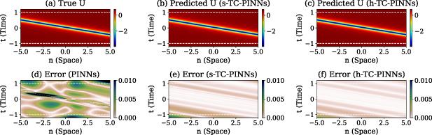
Figure 7. Data-driven first-order RS solution for equation ( |
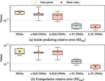
Figure 8. Boxplots of inside predicting and extrapolation relative errors for first-order RS solution with different methods (PINNs, s-SDE-PINNs, h-SDE-PINNs, s-TC-PINNs, h-TC-PINNs) using 5 random seeds per model. |
Table 4. Accuracy and time consumption of numerical simulation for first-order RS solution under different models. Values in bold represent inside predicting and extrapolation relative errors of models with hard constraints, and the training time of h-TC-PINNs is also marked in bold, so as to intuitively compare whether our method achieves superior computational efficiency. |
| Model | $\text{RE}_{\text{Ins}}$ | $\text{RE}_{\text{Ext}}$ | Time |
|---|---|---|---|
| PINNs | $(2.75 \pm 0.52) \times 10^{-3}$ | $(4.67 \pm 1.72) \times 10^{-3}$ | $(139.47\pm22.06)$s |
| s-SDE-PINNs | $(2.56 \pm 1.53) \times 10^{-3}$ | $(4.53 \pm 2.32) \times 10^{-3}$ | $(135.49\pm24.49)$s |
| h-SDE-PINNs | $\mathbf{(1.86 \pm 0.82) \times 10^{-3}}$ | $\mathbf{(4.44 \pm 2.05) \times 10^{-3}}$ | $(162.08\pm28.58)$s |
| s-TC-PINNs | $(5.14 \pm 1.58) \times 10^{-4}$ | $(1.37 \pm 0.37) \times 10^{-3}$ | $(146.76\pm26.94)$s |
| h-TC-PINNs | $\mathbf{(4.30 \pm 1.10) \times 10^{-4}}$ | $\mathbf{(7.35 \pm 1.64) \times 10^{-4}}$ | $\mathbf{(121.84\pm24.49)\mathrm{s}}$ |
4. Parameter inversion of equation (1 )
Table 5. Comparison of parameter inversion results for one-soliton solution under five models and different noise conditions. |
| Model | Condition | Parameter $(\lambda_{1},\lambda_{2})$ | Relative error |
|---|---|---|---|
| Correct | $(1.000\,000,1\,000\,000)$ | $(0.0000,0.0000)$ | |
| | |||
| PINNs | Clean data | $(1.000\,514,0.999\,946)$ | $(5.1400 \times 10^{-4},5.4000 \times 10^{-5})$ |
| 3% noise | $(0.994\,003,0.996\,814)$ | $(5.9970 \times 10^{-3},3.1860 \times 10^{-3})$ | |
| 5% noise | $(0.994\,599,0.995\,671)$ | $(5.4010 \times 10^{-3},4.3290 \times 10^{-3})$ | |
| 10% noise | $(0.862\,656,0.942\,404)$ | $(1.3734 \times 10^{-1},5.7596 \times 10^{-2})$ | |
| | |||
| s-SDE-PINNs | Clean data | $(0.999\,580,0.999\,820)$ | $(4.2000 \times 10^{-4},1.8000 \times 10^{-4})$ |
| 3% noise | $(1.002\,307,0.999\,582)$ | $(6.5600 \times 10^{-3},5.3700 \times 10^{-4})$ | |
| 5% noise | $(1.006\,560,1.000\,537)$ | $(2.3070 \times 10^{-3},4.1800 \times 10^{-4})$ | |
| 10% noise | $(1.012\,264,0.999\,902)$ | $(1.2264 \times 10^{-2},9.8000 \times 10^{-5})$ | |
| | |||
| h-SDE-PINNs | Clean data | $(0.999\,291,0.999\,749)$ | $(7.0900 \times 10^{-4},2.5100 \times 10^{-4})$ |
| 3% noise | $(0.998\,021,0.999\,240)$ | $(1.9700 \times 10^{-3},2.8400 \times 10^{-4})$ | |
| 5% noise | $(0.997\,840,0.999\,375)$ | $(2.1600 \times 10^{-3},6.2500 \times 10^{-4})$ | |
| 10% noise | $(0.999\,912,1.000\,284)$ | $(8.8000 \times 10^{-5},2.8400 \times 10^{-4})$ | |
| | |||
| s-TC-PINNs | Clean data | $0.999\,966,0.999\,940)$ | $(3.4000 \times 10^{-5},6.0000 \times 10^{-5})$ |
| 3% noise | $(1.000\,327,0.999\,887)$ | $(3.2720 \times 10^{-4},1.1320 \times 10^{-4})$ | |
| 5% noise | $(1.000\,138,0.999\,572)$ | $(1.3840 \times 10^{-4},4.2800 \times 10^{-4})$ | |
| 10% noise | $(1.000\,487,0.999\,153)$ | $(4.8660 \times 10^{-4},8.4700 \times 10^{-4})$ | |
| | |||
| h-TC-PINNs | Clean data | $(0.999\,878,1.000\,009)$ | $(1.2200 \times 10^{-4},9.0000 \times 10^{-6})$ |
| 3% noise | $(1.000\,207,0.999\,911)$ | $(2.0700 \times 10^{-4},8.9000 \times 10^{-5})$ | |
| 5% noise | $(1.000\,112,0.999\,744)$ | $(1.1200 \times 10^{-4},2.5600 \times 10^{-4})$ | |
| 10% noise | $(1.000\,896,0.999\,415)$ | $(8.9600 \times 10^{-4},5.8500 \times 10^{-4})$ | |
Table 6. Comparison of parameter inversion results for two-soliton solution under five models and different noise conditions. |
| Model | Condition | Parameter $(\lambda_{1},\lambda_{2})$ | Relative error |
|---|---|---|---|
| Correct | $(1.000\,000,1.000\,000)$ | $(0.0000.0000)$ | |
| | |||
| PINNs | Clean data | $(0.999\,697,1.000\,429)$ | $(3.0300 \times 10^{-4},4.2900 \times 10^{-4})$ |
| 3% noise | $(0.990\,605,0.992\,072)$ | $(9.3950 \times 10^{-3},7.9280 \times 10^{-3})$ | |
| 5% noise | $(0.973\,323,0.984\,313)$ | $(2.6677 \times 10^{-2},1.5687 \times 10^{-2})$ | |
| 10% noise | $(0.907\,931,0.952\,665)$ | $(9.2069 \times 10^{-2},4.7335 \times 10^{-2})$ | |
| | |||
| s-SDE-PINNs | Clean data | $(0.998\,493,0.999\,543)$ | $(1.5070 \times 10^{-3},4.5700 \times 10^{-4})$ |
| 3% noise | $(1.000\,989,0.998\,826)$ | $(9.8900 \times 10^{-4},1.1740 \times 10^{-3})$ | |
| 5% noise | $(1.001\,941,0.998\,916)$ | $(1.9410 \times 10^{-3},1.0840 \times 10^{-3})$ | |
| 10% noise | $(1.004\,893,0.997\,931)$ | $(4.8930 \times 10^{-3},2.0690 \times 10^{-3})$ | |
| | |||
| h-SDE-PINNs | Clean data | $(0.999\,410,0.999\,597)$ | $(5.9000 \times 10^{-4},4.0300 \times 10^{-4})$ |
| 3% noise | $(1.000\,632,0.999\,331)$ | $(6.3200 \times 10^{-4},6.6900 \times 10^{-4})$ | |
| 5% noise | $(1.000\,676,0.998\,904)$ | $(6.7600 \times 10^{-4},1.0960 \times 10^{-3})$ | |
| 10% noise | $(1.003\,399,0.998\,338)$ | $(3.3990 \times 10^{-3},1.6620 \times 10^{-3})$ | |
| | |||
| s-TC-PINNs | Clean data | $(1.000\,395,1.000\,034)$ | $(3.9500 \times 10^{-4},3.4000 \times 10^{-5})$ |
| 3% noise | $(0.999\,385,0.999\,161)$ | $(6.1500 \times 10^{-4},8.3900 \times 10^{-4})$ | |
| 5% noise | $(0.999\,279,0.998\,446)$ | $(7.2100 \times 10^{-4},1.5540 \times 10^{-3})$ | |
| 10% noise | $(0.999\,217,0.997\,335)$ | $(7.8300 \times 10^{-4},2.6550 \times 10^{-3})$ | |
| | |||
| h-TC-PINNs | Clean data | $(0.999\,743,0.999\,870)$ | $(2.5700 \times 10^{-4},1.3000 \times 10^{-4})$ |
| 3% noise | $(0.999\,390,0.999\,092)$ | $(6.1000 \times 10^{-4},9.0800 \times 10^{-4})$ | |
| 5% noise | $(0.998\,459,0.998\,205)$ | $(1.5410 \times 10^{-3},1.7950 \times 10^{-3})$ | |
| 10% noise | $(0.997\,753,0.996\,620)$ | $(2.2470 \times 10^{-3},3.3800 \times 10^{-3})$ | |
Table 7. Comparison of parameter inversion results for first-order RS solution under five models and different noise conditions. |
| Model | Condition | Parameter $(\lambda_{1},\lambda_{2})$ | Relative error |
|---|---|---|---|
| Correct | $(1.000\,000,1.000\,000)$ | $(0.0000,0.0000)$ | |
| | |||
| PINNs | Clean data | $(0.998\,249,1.000\,733)$ | $(1.7510 \times 10^{-4},7.3300 \times 10^{-4})$ |
| 3% noise | $(1.001\,975,1.004\,498)$ | $(1.9750 \times 10^{-3},4.4980 \times 10^{-3})$ | |
| 5% noise | $(0.989\,970,0.992\,871)$ | $(1.0030 \times 10^{-2},7.1290 \times 10^{-3})$ | |
| 10% noise | $(0.877\,464,0.922\,756)$ | $(1.2254 \times 10^{-1},7.7244 \times 10^{-2})$ | |
| | |||
| s-SDE-PINNs | Clean data | $(1.000\,043,1.000\,119)$ | $(4.3400 \times 10^{-4},2.1190 \times 10^{-3})$ |
| 3% noise | $(0.998\,565,0.998\,770)$ | $(1.4350 \times 10^{-3},1.2300 \times 10^{-4})$ | |
| 5% noise | $(0.999\,976,0.999\,822)$ | $(8.4000 \times 10^{-5},1.7800 \times 10^{-4})$ | |
| 10% noise | $(0.997\,193,0.999\,446)$ | $(2.8070 \times 10^{-3},5.5400 \times 10^{-4})$ | |
| | |||
| h-SDE-PINNs | Clean data | $(1.002\,695,0.999\,122)$ | $(2.6950 \times 10^{-3},7.8400 \times 10^{-4})$ |
| 3% noise | $(1.012\,460,1.002\,166)$ | $(1.2460 \times 10^{-2},2.1660 \times 10^{-3})$ | |
| 5% noise | $(0.998\,538,0.999\,106)$ | $(1.4620 \times 10^{-3},8.9400 \times 10^{-4})$ | |
| 10% noise | $(1.002\,766,0.999\,035)$ | $(2.6660 \times 10^{-3},9.6500 \times 10^{-4})$ | |
| | |||
| s-TC-PINNs | Clean data | $(1.000\,459,1.000\,326)$ | $(4.5900 \times 10^{-4},3.2600 \times 10^{-4})$ |
| 3% noise | $(1.000\,477,1.000\,435)$ | $(4.7700 \times 10^{-4},4.3500 \times 10^{-4})$ | |
| 5% noise | $(1.000\,445,1.000\,494)$ | $(4.4500 \times 10^{-4},4.9400 \times 10^{-4})$ | |
| 10% noise | $(1.000\,720,1.000\,587)$ | $(7.2000 \times 10^{-4},5.8700 \times 10^{-4})$ | |
| | |||
| h-TC-PINNs | Clean data | $(1.000\,538,1.000\,215)$ | $(5.3800 \times 10^{-4},2.1500 \times 10^{-4})$ |
| 3% noise | $(1.000\,346,1.000\,330)$ | $(3.4600 \times 10^{-4},3.3000 \times 10^{-4})$ | |
| 5% noise | $(1.000\,646,1.000\,446)$ | $(6.4600 \times 10^{-4},4.4600 \times 10^{-4})$ | |
| 10% noise | $(1.000\,131,1.000\,595)$ | $(1.3100 \times 10^{-4},5.9500 \times 10^{-4})$ | |
5. Ablation experiments and parameter sensitivity analysis
5.1. Selection of activation function
Table 8. Performance comparison with different activation functions. |
| Activation function | $\text{RE}_{\text{Ins}}$ | $\text{RE}_{\text{Ext}}$ |
|---|---|---|
| Tanh | $(2.11 \pm 0.95)\times 10^{-4}$ | $(4.01 \pm 1.36)\times 10^{-3}$ |
| Sin | $(2.24 \pm 0.79)\times 10^{-4}$ | $(5.35 \pm 2.15)\times 10^{-3}$ |
| ReLU | $(1.34 \pm 0.55)\times 10^{-1}$ | $(4.75 \pm 1.65)\times 10^{-1}$ |
| SiLU | $(2.11 \pm 0.74)\times 10^{-4}$ | $(4.92 \pm 1.66)\times 10^{-3}$ |
| Sigmoid | $(2.14 \pm 0.72)\times 10^{-4}$ | $(3.52 \pm 1.25)\times 10^{-3}$ |
5.2. Selection of network architecture
Table 9. Performance under different network depths and widths (h-TC-PINNs vs. PINNs). |
| Depth | Width | h-TC-PINNs | PINNs | ||
|---|---|---|---|---|---|
| $\text{RE}_{\text{Ins}}$ | $\text{RE}_{\text{Ext}}$ | $\text{RE}_{\text{Ins}}$ | $\text{RE}_{\text{Ext}}$ | ||
| 2 | 16 | $1.2306 \times 10^{-4}$ | $2.8053 \times 10^{-3}$ | $1.5685 \times 10^{-4}$ | $4.0075 \times 10^{-3}$ |
| 32 | $1.7000 \times 10^{-4}$ | $3.3711 \times 10^{-3}$ | $5.0491 \times 10^{-4}$ | $1.0152 \times 10^{-2}$ | |
| 64 | $2.2712 \times 10^{-4}$ | $4.9042 \times 10^{-3}$ | $4.2500 \times 10^{-4}$ | $7.2540 \times 10^{-3}$ | |
| | |||||
| 4 | 16 | $1.1468 \times 10^{-4}$ | $2.0748 \times 10^{-3}$ | $4.3244 \times 10^{-4}$ | $6.7950 \times 10^{-3}$ |
| 32 | $2.3491 \times 10^{-4}$ | $4.9491 \times 10^{-3}$ | $5.2000 \times 10^{-4}$ | $7.2580 \times 10^{-3}$ | |
| 64 | $2.1359 \times 10^{-4}$ | $4.1940 \times 10^{-3}$ | $6.4000 \times 10^{-4}$ | $1.2342 \times 10^{-2}$ | |
| | |||||
| 6 | 16 | $2.2858 \times 10^{-4}$ | $4.5635 \times 10^{-3}$ | $1.2630 \times 10^{-3}$ | $1.8837 \times 10^{-2}$ |
| 32 | $2.0512 \times 10^{-4}$ | $3.9888 \times 10^{-3}$ | $6.0300 \times 10^{-4}$ | $1.1938 \times 10^{-2}$ | |
| 64 | $1.3145 \times 10^{-4}$ | $1.8964 \times 10^{-3}$ | $6.7500 \times 10^{-4}$ | $1.0223 \times 10^{-2}$ | |
5.3. Selection of loss weights
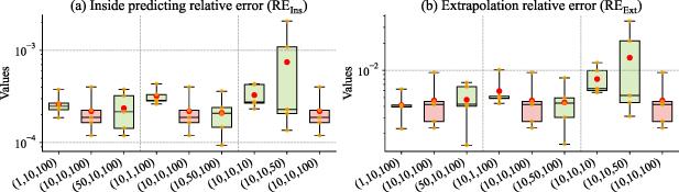
Figure 9. Box plots of inside predicting and extrapolation relative errors of the h-TC-PINNs method under different loss weights. |
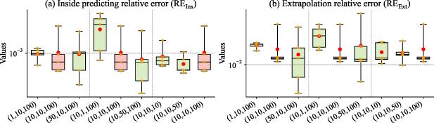
Figure 10. Box plots of inside predicting and extrapolation relative errors of the PINNs method under different loss weights. |
5.4. Basis for time step $\Delta t$ selection and its influence on hard constraints
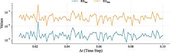
Figure 11. Inside predicting and extrapolation relative errors under different time steps. |
Table 10. Correlation analysis between time step and prediction errors. |
| Metric | $\text{RE}_{\text{Ins}}$ | $p$-value | $\text{RE}_{\text{Ext}}$ | $p$-value |
|---|---|---|---|---|
| Pearson correlation ($r$) | $-0.110$ | $0.2745$ | $-0.112$ | $0.2677$ |
| Spearman correlation ($r$) | $-0.027$ | $0.7928$ | $-0.040$ | $0.6916$ |
| Coefficient of determination ($R^2$) | $0.012$ | — | $0.013$ | — |
5.5. Fairness verification of traveling wave transformation
Table 11. Performance comparison of different models. |
| Model | $\text{RE}_{\text{Ins}}$ | $\text{RE}_{\text{Ext}}$ |
|---|---|---|
| PINNs | $(8.32 \pm 1.13)\times 10^{-4}$ | $(1.32 \pm 0.21)\times 10^{-2}$ |
| PINNs+$v_m$ | $(7.95 \pm 3.43)\times 10^{-4}$ | $(2.21 \pm 1.27)\times 10^{-2}$ |
| h-TC-PINNs | $(2.11 \pm 0.95)\times 10^{-4}$ | $(4.01 \pm 1.36)\times 10^{-3}$ |
5.6. Applicability analysis under unknown $v_m$
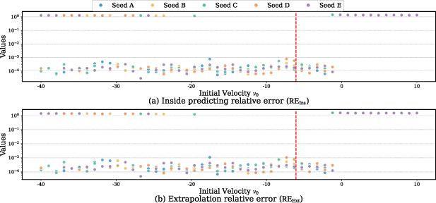


Figure 12. Inside predicting and extrapolation relative errors under different initial velocities. The red dashed line marks the position of the true velocity. |
6. Conclusions
| • Significant improvement in the accuracy of predicted solutions: the proposed TC-PINNs are first applied to the numerical simulation of ordinary soliton solution (one-soliton solution, two-soliton solution), and then extended to the scenario of RS solution (first-order RS solution). The relative error of internal prediction of the model is reduced to the order of $10^{-4}$ for all cases, achieving a substantial improvement in the accuracy of predicted solutions. Moreover, h-TC-PINNs demonstrate even higher prediction accuracy. | |
| • Excellent extrapolation and generalization capability: this method has demonstrated outstanding extrapolation performance in the simulation of ordinary soliton solution (one-soliton solution, two-soliton solution), with the extrapolation error reduced by 30%–50% compared with traditional PINNs. When extended to RS solution (first-order RS solution), the model still maintains stable extrapolation accuracy, effectively breaking through the generalization bottleneck of data-driven methods in the extrapolation task of discrete systems, and reflecting the universal generalization ability of the constraint-enhanced mechanism for different types of soliton solutions. Furthermore, h-TC-PINNs exhibit stronger generalization robustness. | |
| • Superior performance in parameter inversion: the proposed constraint-based model exhibits outstanding performance in parameter inversion tasks for all types of soliton solutions. In the parameter inversion of one-soliton solution, two-soliton solution and first-order RS solution, even under the interference of 10% Gaussian noise, the relative inversion error is still controlled within the order of $10^{-3}$–$10^{-4}$, which is significantly better than traditional PINNs, fully verifying the reliability and robustness of the proposed method in parameter inversion. |