

1. Introduction
The study of two-dimensional (2D) systems plays a key role in the understanding of a vast array of physical phenomena, including topological orders, superconductivity and superfluidity, quantum magnetism, and unconventional non-equilibrium processes. Owing to the unprecedented controllability, ultracold quantum gases of atoms provide a versatile platform to investigate 2D and quasi-2D systems. In continuum gases, a 2D Bose–Einstein condensate has been realized to reveal characteristic features of the Kosterlitz–Thouless transition [1–5], critical velocity [6], collective modes [7–9], dynamics [10–12], and Kibble–Zurek mechanism [13], while 2D Fermi gases have also been created with equal [14, 15] and unequal [16, 17] spin populations to study the crossover from the weakly interacting Bardeen–Cooper–Schrieffer state to the Bose–Einstein condensate (BEC) regime of bound molecules [18–20], sound wave transport [21, 22], superfluid properties [23–25], vortex dynamics [26], and polaron physics [27, 28].
Despite promising progress in experiments, cold atomic gases are inherently metastable with a rather limited lifetime. One of the most significant limitations to their lifetime is three-body loss, through which three free atoms collide to form a deeply bound dimer and an atom carrying excess energy to escape from the trap [29]. This process, characterized by a three-body recombination rate $K_3$, plays an important role not only in the stability of quantum gases [30, 31], but also in the study of the exotic Efimov effect [31, 32], where resonant three-body bound states appear even when two-body states are absent [33, 34]. While properties of three-body physics in three dimensions have been extensively studied [35–42], 2D and quasi-2D geometries bring in unique challenges, such as the logarithmic dependence [43, 44] of scattering amplitude on energy and the strong effect of quantum fluctuations [45–47]. Previous work in this direction includes the study of three-body scattering in 2D systems [48], and extension to atomic gases [49–51]. Nevertheless, an exact solution of atom-dimer scattering amplitude and its application in three-body recombination remain incomplete.
In this work, we investigate the three-body scattering processes within distinguishable particles in 2D continuous systems and calculate the three-body loss rate by the framework of Skorniakov–Ter-Martirosian (STM) equations. Originally developed for three-nucleon systems [52], STM equations allow for the exact treatment of atom-dimer scattering by reducing the three-body Schrödinger equation into a set of coupled integral equations in relative coordinates. We first generalize the STM equations to two dimensions, and compute the scattering states from different incoming states. By considering an initial state with zero center-of-mass momentum, we calculate the atom-dimer scattering amplitude $f_\mathrm{ad}$ with varying interaction strength and mass ratio in comparison to those obtained from mean-field theory (MFT) and single-pole approximation (SPA). We find that while both approximations work well in the limit of weak interaction, SPA provides a satisfactory result with a relative error of only one percent within a much wider interaction range. Then, we discuss the problem of three-body recombination with three free particles being scattered into a dimer and an atom, and obtain the scattering $T$-matrix and an estimation of the lifetime of the quantum gas. We find that the lifetime nearly depends on the 2D gas parameter in a power law with an exponent ${\sim}- 2.45$. These results can provide useful information for future experimental studies of few-body physics and quantum gases in two dimensions.
2. STM equations and scattering amplitude
Owing to the nature of diluteness, the low-energy physics in ultracold atomic gases is mostly governed by few-body processes. The scattering amplitude, in direct connection with the scattering cross section, encodes a wealth of physical observables. For two-body problems, scattering theories have been well developed for both elastic and inelastic channels with the notion of Lippmann–Schwinger (LS) equation. As for three-body processes, STM-equation approach is widely employed to treat problems including deuteron-nucleon scattering, Efimov states, atom-dimer scattering, and three-body loss near a Feshbach resonance. It exhibits great potential for solving scattering amplitudes across systems of different dimensions [42, 52, 53]. Next, we formulate STM equations in two dimensions and derive an equation for an auxiliary function $f(K)$, which converges to the atom-dimer scattering amplitude $f_\mathrm{ad}$ in the limit of zero atom-dimer relative momentum ${\boldsymbol{K}}\to 0^+$. The result is then compared with that obtained with MFT and SPA. We find that while MFT only works in the weakly interacting limit, SPA behaves quite well in a much wider range of interaction considered in this work, which is starkly different from three-dimensional systems.
2.1. STM equations
We consider the three-body scattering process in a gas mixture of two species, as schematically illustrated in figure 1. One species has two components, or equivalently, pseudo-spins, as labeled by atoms 1 and 2 (blue) with dimensionless masses $m_1 = m_2 = 1 $, while the other species is labeled by atom 3 (red) with mass $m_3 = M$. To describe the relative motion between the atoms, we adopt the relative-momentum representation, with relative-momentum operators $\hat{\boldsymbol{k}}_{12} = (\hat{\boldsymbol{k}}_1 - \hat{\boldsymbol{k}}_2)/2$, $\hat{\boldsymbol{K}}_{3{\textrm{-}}12} = [2\hat{\boldsymbol{k}}_3 - M(\hat{\boldsymbol{k}}_{1} +\hat{\boldsymbol{k}}_{2})] /(2+M)$, and the total momentum $ \hat{\boldsymbol{K}} _\mathrm{tot} = \hat{\boldsymbol{k}}_1 +\hat{\boldsymbol{k}}_2 +\hat{\boldsymbol{k}}_3$. In the following discussion, the total momentum is assumed to be zero, $\boldsymbol{K}_\mathrm{tot} = 0 $, to respect the translational symmetry of a continuous space unless specified. Within the basis of relative momenta satisfying the eigen-equations $\hat{\boldsymbol{k}}_{ij} \ket{\boldsymbol{k}_0}_{ij} = \boldsymbol{k}_0\ket{\boldsymbol{k}_0}_{ij} $ and $\hat{\boldsymbol{K}}_{k{\textrm{-}}ij} \ket{\boldsymbol{K}_0}_{k{\textrm{-}}ij} = \boldsymbol{K}_0\ket{\boldsymbol{K}_0}_{k{\textrm{-}}ij} $, the Hamiltonian of the system can be separated into a kinetic term and an interaction term $\hat{H} = \hat{H}_0 + \hat{V}$. The kinetic term is
$\begin{align} \hat{H}_0 = \sum_{i} \frac{\hat{\boldsymbol{k}}_i^2}{2 m_i } = \frac{\hat{\boldsymbol{k}}_{ij}^2}{2 m_{ij} } + \frac{\hat{\boldsymbol{K}}_{k{\textrm{-}}ij}^2}{2 m_{k{\textrm{-}}ij} },\end{align}$
where $(ijk)$ takes $(123)$, $(231)$ and $(312)$, $m_{ij}$ denotes the reduced mass of atoms $i$ and $j$, $m_{k{\textrm{-}}ij}$ is the reduced mass of atom $k$ relative to the center-of-mass of atoms $i$ and $j$, and $\hbar = 1$ in the natural unit.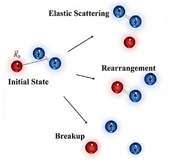
Figure 1. Schematic illustration of the three-body scattering process. The initial state (left) consists of a dimer and a free atom with momentum $\boldsymbol{K}_0$ relative to the dimer. Three possible scattering channels include: elastic atom-dimer scattering that preserves the original dimer (top), inelastic scattering that rearranges the dimer with a different atomic composition (middle), and breakup that results in three free atoms (bottom). |
To address the problem of atom-dimer scattering, we consider an incoming state $\ket*{\Psi_{\boldsymbol{K}_0}^\textrm{in}} = \ket{\phi_b}_{12} \ket{\boldsymbol{K}_0}_{3{\textrm{-}}12}$ composed of a two-body bound state formed by atoms 1 and 2 ($\ket{\phi_b}_{12}$) and a free atom 3 with relative momentum ${\boldsymbol{K}_0}$ ($\ket{\boldsymbol{K}_0}_{3{\textrm{-}}12}$). The scattering state $\ket*{\Psi_{\boldsymbol{K}}^{(+)}}$ is described by the LS equation
$\begin{align} \ket*{\Psi_{\boldsymbol{K}}^{\left(+\right)}} & = \lim_{\varepsilon \to 0^+} \frac{\textrm{i}\varepsilon}{E+\textrm{i}\varepsilon- \hat{H}} \ket*{\Psi_{\boldsymbol{K}_0}^\textrm{in}} \nonumber \\ & = \textrm{i}\varepsilon \hat{G}_{0} \ket*{\Psi_{\boldsymbol{K}_0}^\textrm{in}} + \hat{G}_{0} \hat{V} \ket*{\Psi_{\boldsymbol{K}}^{\left(+\right)}},\end{align}$
where the free Green’s function is defined as $\hat{G}_{0} = (E + \textrm{i}\varepsilon -\hat{H}_{0})^{-1}$ and the corresponding energy $E = -E_{12} + {(M+2)} K_0^2/{4M} $. The interaction potential $V = V_{12}+V_{23}+V_{31}$ consists of two-body contact interactions between any two atoms, and can be represented in momentum space as $\begin{align}V_{12} & = \frac{g_{12}}{\left(2\pi\right)^2} \int \mathrm{d}\boldsymbol{k} \mathrm{d}\boldsymbol{k^{^{\prime}}} \ket{\boldsymbol{k}}_{12} \bra{\boldsymbol{k^{^{\prime}}}} = g_{12}\ket{\phi}_{12} \bra{\phi}, \nonumber \\ V_{23} & = \frac{g_{23}}{\left(2\pi\right)^2} \int \mathrm{d}\boldsymbol{k} \mathrm{d}\boldsymbol{k^{^{\prime}}} \ket{\boldsymbol{k}}_{23} \bra{\boldsymbol{k^{^{\prime}}}} = g_{23} \ket{\phi}_{23} \bra{\phi}, \nonumber \\ V_{31} & = \frac{g_{31}}{\left(2\pi\right)^2} \int \mathrm{d}\boldsymbol{k} \mathrm{d}\boldsymbol{k^{^{\prime}}} \ket{\boldsymbol{k}}_{31} \bra{\boldsymbol{k^{^{\prime}}}} = g_{31} \ket{\phi}_{31} \bra{\phi}.\end{align}$
Here, we use the symmetry of $g_{31} = g_{23}$ and define $\ket{\phi}_{ij} \equiv \int {\mathrm{d}\boldsymbol{k}}\ket{\boldsymbol{k}}_{ij}/{2\pi} $. Given the equivalence of atoms 1 and 2 in both the initial state and the Hamiltonian, we introduce two wave functions $\eta$ and $\chi$ by applying the interaction potentials to the scattering state, reading $\begin{align}V_{12} \ket*{\Psi_{\boldsymbol{K}}^{\left(+\right)}} & = \ket*{\phi}_{12} \ket{\eta}_{3{\textrm{-}}12},\nonumber\\ V_{23} \ket*{\Psi_{\boldsymbol{K}}^{\left(+\right)}} & = \ket*{\phi}_{23} \ket{\chi}_{1{\textrm{-}}23},\nonumber\\ V_{31} \ket*{\Psi_{\boldsymbol{K}}^{\left(+\right)}} & = \ket*{\phi}_{31} \ket{\chi}_{2{\textrm{-}}31}.\end{align}$
By acting $\left({1}/{g_{12}} \right) _{3{\textrm{-}}12}\bra{\boldsymbol{K}}_{12}\bra*{\phi_b}V_{12}$ on both sides of equation (2 ), we obtain
$\begin{align} &\left( \frac{1}{4\pi} \log{\frac{E_{12}}{\frac{M+2}{4M} K^2 -E -\textrm{i}\varepsilon}} \right) \eta\left(\boldsymbol{K}\right)\nonumber\\ &\quad = \int \frac{\mathrm{d}\boldsymbol{K}^{^{\prime}}}{\left(2\pi\right)^2} \frac{2 \chi\left(\boldsymbol{K^{^{\prime}}}\right)}{E+\textrm{i}\varepsilon -K^{^{\prime} 2} -\frac{M+1}{2M}K^2 -\boldsymbol{K \cdot K^{^{\prime}}}} \nonumber \\ & \qquad -\frac{\textrm{i}\varepsilon \sqrt{E_{12}}} {2\sqrt{\pi}} \frac{\delta\left(\boldsymbol{K} - \boldsymbol{K}_0\right)} {\textrm{i}\varepsilon -\frac{M+2}{4M} K_0^2} \log{\frac{E_{12}} {\frac{M+2}{4M}K_0^2 - E -\textrm{i}\varepsilon}},\end{align}$
from which we can solve the scattering state with the help of functions $\eta$ and $\chi$. Here, we impose the expression of the bare interaction strengths $g_{12}$ and $g_{23}$, satisfying the following 2D renormalization relation $\begin{align} \frac{1}{g_{12}}& = -\frac{1}{\left(2\pi\right)^2}\int\frac{\mathrm{d}\boldsymbol{k}}{k^2+E_{12}}, \nonumber \\ \frac{1}{g_{23}}& = -\frac{1}{\left(2\pi\right)^2}\int\frac{2M}{M+1} \frac{\mathrm{d}\boldsymbol{k}}{k^2+E_{23}},\end{align}$
and the bound state wave function $\begin{align} \phi_b\left(\boldsymbol{k}\right) = \sqrt{\frac{E_{12}}{\pi}} \frac{1}{k^2+E_{12}},\end{align}$
as derived in appendix $\begin{align} \eta\left(\boldsymbol{K}\right) &\equiv -\frac{2\sqrt{\pi E_{12}}} {\left(2\pi\right)^2 } \left[ \left(2\pi\right)^2 \delta\left(\boldsymbol{K} - \boldsymbol{K}_0 \right) + \frac{f\left(\boldsymbol{K}\right)} {\frac{4M}{M+2} \textrm{i}\varepsilon -K^2} \right], \nonumber \\ \chi\left(\boldsymbol{K}\right)&\equiv-\frac{2\sqrt{\pi E_{12}}}{\left(2\pi\right)^2 }\zeta\left(\boldsymbol{K}\right),\end{align}$
where $f(\boldsymbol{K})$ is related to the atom-dimer scattering amplitude by $\lim_{\boldsymbol{K} \to 0} f(\boldsymbol{K}) = f_\mathrm{ad} $ as proven in appendix $\begin{align} \log{\frac{E_{12}} {\frac{M+2}{4M} K^2 + E_{12} }} \frac{f\left(\boldsymbol{K}\right)} {K^2} = \int \frac{\mathrm{d}\boldsymbol{K}^{^{\prime}}}{\pi} \frac{2\zeta\left(\boldsymbol{K}^{^{\prime}}\right)} {K^{^{\prime} 2} + \frac{M+1}{2M} K^2 + \boldsymbol{K \cdot K^{^{\prime}}} + E_{12}}.\end{align}$
The second STM equation is derived by multiplying $\left(1/g_{23}\right) _{2{\textrm{-}}31}\bra{\boldsymbol{K}}_{31}\bra*{\phi_b}V_{31}$ on equation ( $\begin{align} &\left[\frac{2\pi M}{M+1} \log{\frac{\frac{M+1}{2M}E_{23}} {\frac{M+2}{4M}K^2 +E_{12} }} \right] \zeta\left(\boldsymbol{K}\right) - \frac{4\pi}{K^2 +E_{12}} \nonumber\\ &\qquad +\int \frac{\mathrm{d}\boldsymbol{K}^{^{\prime}} }{K^{^{\prime} 2} +\frac{M+1}{2M}K^2 +\boldsymbol{K \cdot K^{^{\prime}}} +E_{12}} \frac{f\left(\boldsymbol{K}^{^{\prime}}\right)}{K^{^{\prime} 2} } \nonumber \\ &\quad = \int \frac{\mathrm{d}\boldsymbol{K}^{^{\prime}} \zeta\left(\boldsymbol{K}^{^{\prime}}\right)} {K^{^{\prime} 2}+\frac{M+1}{2M}K^2+\frac{1}{M}\boldsymbol{K \cdot K^{^{\prime}}} +E_{12}}.\end{align}$
For further simplification, we exploit the rotational symmetry to write $f(\boldsymbol{K^{^{\prime}}}) = f(K^{^{\prime}})$ and $\zeta(\boldsymbol{K^{^{\prime}}}) = \zeta(K^{^{\prime}})$, and obtain the full STM equations as $\begin{align} &\log{\frac{E_{12}} {\frac{M+2}{4M}K^2 +E_{12}}} \frac{f\left(K\right)}{K^2} \nonumber\\ &\quad =\int_{0}^{+\infty} \frac{4K^{^{\prime}}\mathrm{d} K^{^{\prime}}\zeta\left(K^{^{\prime}}\right)}{\sqrt{\left(K^{^{\prime} 2} +\frac{M+1}{2M}K^2 +E_{12}\right)^2 - K^2K^{^{\prime} 2}}}, \nonumber \\ &\log{\frac{E_{23}} {\frac{M+2}{4M}K^2 +E_{12}}}\zeta\left(K\right)\nonumber\\ &\quad = \frac{4\pi}{K^2+E_{12}} -\int_{0}^{+\infty} \frac{\mathrm{d} K^{^{\prime}}}{K^{^{\prime}}} \frac{f\left(K^{^{\prime}}\right)}{\sqrt{\left( \frac{M+1}{2M}K^{^{\prime} 2} +K^2 +E_{12}\right)^2 - K^2 K^{^{\prime} 2}}} \nonumber \\ &\quad\quad +\int_{0}^{+\infty} \frac{2K^{^{\prime}}\mathrm{d} K^{^{\prime}}\zeta\left(K^{^{\prime}}\right)}{\sqrt{\left(\frac{M+1}{2M}K^{^{\prime} 2} +K^2 +E_{12}\right)^2 - \left(K K^{^{\prime}}/M\right)^2 }}.\end{align}$
The scattering amplitude $f_\textrm{ad}$ can be obtained by solving these two coupled equations.2.2. Comparison to MFT and SPA
The scattering amplitude in the mean-field level can be obtained from the Born approximation. We first expand the scattering state into Born series C , the scattering $T$-matrix $\bra{\Psi_{\text{in}}} (V_{23} + V_{31}) \ket{\Psi_{\text{in}}} $ under Born approximation reads
$\begin{align} \ket{\Psi_+} & = \ket{\Psi_{\text{in}}} + G_0 V \ket{\Psi_+} \nonumber \\ & = \ket{\Psi_{\text{in}}} + G_0 V \left( \ket{\Psi_{\text{in}}} + G_0 V \ket{\Psi_+} \right) + \dots,\end{align}$
where the lowest order gives $\ket{\Psi_+} = \ket{\Psi_{\text{in}}}$. Under the Jacobi transformation of the basis given in appendix $\begin{equation} \bra{\Psi_{\text{in}}} \left(V_{23} + V_{31}\right) \ket{\Psi_{\text{in}}} = \frac{2g_{\text{23}}}{\left(2\pi\right)^2},\end{equation}$
where the mean-field interaction strength is $\begin{equation}g_{\text{23}} = \frac{2\hbar^2 \pi}{m_{\text{23}}} \frac{1}{\log\left(E_{\text{23}}/E_{12}\right)}.\end{equation}$
With that, the scattering amplitude in MFT becomes $\begin{equation} f_{\text{ad}}^{\,\,0} = \frac{8\pi m_{\text{ad}}}{m_{\text{23}}} \frac{1}{\log\left(E_{23}/E_{12}\right)}.\end{equation}$
In figure 2, we display the difference between the result obtained from STM equations and that from MFT for different mass ratios, as a function of interaction strength. Notice that the discrepancy increases with mass ratio, and saturates to a finite value depending on interaction. This implies that a heavier atom would suppress the dissociation of the dimer and lead to a higher probability of entering the atom-dimer scattering channel [54].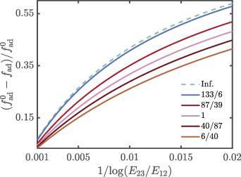
Figure 2. Deviation of atom-dimer scattering amplitude between MFT $f_\textrm{ad}^0$ and the exact solution from STM equations $f_\textrm{ad}$. The mass ratio between the two atom species is tuned from 6/40 to 133/6, and approaches to limiting case of $M \to \infty$. While tuning the inter-species interaction strength $g_{23} \propto {1}/{\log(E_{23} /E_{12})} $ to the weakly interacting limit, the MFT agrees well with the STM equations. When the interaction increases, the deviation is bounded by the dashed line with infinite mass ratio $M$, implying the validity of MFT for mild interaction. |
The SPA assumes that the dimer composed of atoms 1 and 2 will not break during the scattering process. The deviation of SPA clearly displays the contribution of intra-dimer interaction as illustrated in figure 1, which affects the atom-dimer scattering amplitude indirectly via the rearrangement and breakup of the dimer. To see this, we first write the LS equation as
$\begin{equation} \ket*{\Psi_{\boldsymbol{K}}^{\left(+\right)}} = \textrm{i}\varepsilon G_{3}\ket*{\Psi_{\boldsymbol{K}_0}^\mathrm{in}} + G_{3} \left(V_{23}+V_{31}\right) \ket*{\Psi_{\boldsymbol{K}}^{\left(+\right)}} ,\end{equation}$
where the Green’s function is $\begin{align}G_3 & = \int\mathrm{d}{\boldsymbol{K}} \frac{\ket{\boldsymbol{K}}_{3{\textrm{-}}12}\bra{\boldsymbol{K}} \otimes\ket{\phi_b}_{12}\bra{\phi_b}}{\textrm{i}\varepsilon - \left(\frac{M+2}{4M}\right)K^2} \nonumber \\ &\quad + \int \mathrm{d}{\boldsymbol{K}} \mathrm{d}{\boldsymbol{k}} \frac{\ket{\boldsymbol{K}}_{3{\textrm{-}}12}\bra{\boldsymbol{K}} \otimes \ket{\boldsymbol{k}}_{12} \bra{\boldsymbol{k}}}{-E_{12} + \textrm{i}\varepsilon -\left(\frac{M+2}{4M}\right)K^2 -k^2 }.\end{align}$
The SPA is applied by projecting $G_3$ onto the subspace $I _{3{\textrm{-}}12} \otimes \ket{\phi_b}_{12}\bra{\phi_b}$, and neglecting the continuum contribution from the unbound 12 states, leading to $\begin{align} G_3 \approx \int\mathrm{d}{\boldsymbol{K}} \frac{\ket{\boldsymbol{K}}_{3{\textrm{-}}12}\bra{\boldsymbol{K}} \otimes\ket{\phi_b}_{12}\bra{\phi_b}}{\textrm{i}\varepsilon - \left(\frac{M+2}{4M}\right)K^2}.\end{align}$
The scattering state can be easily described as $\ket*{\Psi_{\boldsymbol{K}}^{(+)}} = \ket{\psi}_{3{\textrm{-}}12}\ket{\phi_b}_{12}$, maintaining the dimer throughout the scattering process.To solve for the scattering state $\ket*{\psi}_{3{\textrm{-}}12}$, we multiply $_ {3{\textrm{-}}12}\bra{\boldsymbol{K}} _{12}\bra{\phi_b}$ on both sides of equation (16 ) and directly obtain $ \psi(\boldsymbol{K}) = \delta(\boldsymbol{K}) + \ _{3{\textrm{-}}12}\bra{\boldsymbol{K}} _{12}\bra{\phi_b} G_3 (V_{23}+V_{31}) \ket{\psi}_{3{\textrm{-}}12} \ket{\phi_b}_{12}$. Substitute the expression of $G_3$, we then find that the second term of the equation above relates to the scattering $T$-matrix $T(\boldsymbol{K}) \equiv \ _{3{\textrm{-}}12}\bra{\boldsymbol{K}} _{12}\bra{\phi_b} (V_{23}+V_{31}) \ket{\Psi_{\boldsymbol{K}}^{+}}$ via 16 ) to obtain
$\begin{align} \frac{T\left(\boldsymbol{K}\right)}{\textrm{i}\varepsilon - \left(\frac{M+2}{4M}\right)K^2} = \,_{3 {\textrm{-}} 12}\bra{\boldsymbol{K}} _{12}\bra{\phi_b} G_3 \left(V_{23}+V_{31}\right) \ket{\psi}_{3 {\textrm{-}} 12} \ket{\phi_b}_{12}.\end{align}$
To investigate the exact form of $T(\boldsymbol{K})$, we apply $_ {3 {\textrm{-}} 12}\bra{\boldsymbol{K}}_{12}\bra{\phi_b} (V_{23}+V_{31}) $ on both sides of equation ( $\begin{align}T\left(\boldsymbol{K}\right) & = \int \mathrm{d}{\boldsymbol{K}^{^{\prime}}} _{12}\bra{\phi_b} _{3 {\textrm{-}}12}\bra{\boldsymbol{K}} \left(V_{23}+V_{31}\right) \ket{\boldsymbol{K}^{^{\prime}}}_{3 {\textrm{-}}12}\ket{\phi_b}_{12} \nonumber \\ &\quad \times \left[ \delta\left(\boldsymbol{K}^{^{\prime}}\right) + \frac{T\left(\boldsymbol{K^{^{\prime}}}\right)}{\textrm{i}\varepsilon - \left(\frac{M+2}{4M}\right)K^{^{\prime} 2}} \right] .\end{align}$
For simplicity, we introduce the interaction potential under 3–12 Jacobi basis frame as in appendix C , which leads to $_ {12}\bra{\phi_b} _{3 {\textrm{-}}12}\bra{\boldsymbol{K}} (V_{23}+V_{31}) \ket{\boldsymbol{K}^{^{\prime}}}_{3 {\textrm{-}} 12} \ket{\phi_b}_{12} = {g_{23}}/({2\pi^2}) \int \mathrm{d}\boldsymbol{K^{^{\prime\prime}}} \phi_b( \boldsymbol{K}/2 + \boldsymbol{K^{^{\prime\prime}}}) \phi_b( \boldsymbol{K}^{^{\prime}}/2 +\boldsymbol{K^{^{\prime\prime}}}) $. The LS equation under SPA can be expressed in terms of the bound state wave function $\phi_b(\boldsymbol{k}) $ and the function $h(\boldsymbol{K}) \equiv \lim_{\varepsilon \to 0^+} \frac{T(\boldsymbol{K^{^{\prime}}})} {\textrm{i}\varepsilon - (\frac{M+2}{4M})K^{^{\prime} 2}}$, where the $T$-matrix reads
$\begin{align}T\left(\boldsymbol{K}\right) & = \frac{g_{23}}{2\pi^2} \int\mathrm{d}\boldsymbol{K^{\prime}} \mathrm{d}\boldsymbol{K^{^{\prime\prime}}} \left[ \delta\left(\boldsymbol{K}^{\prime}\right) + h\left(\boldsymbol{K^{\prime}}\right) \right] \nonumber\\ &\quad \times \phi_b\left( \frac{1}{2} \boldsymbol{K} +\boldsymbol{K{^{\prime\prime}}}\right) \phi_b \left( \frac{1}{2} \boldsymbol{K}^{\prime} +\boldsymbol{K{^{\prime\prime}}} \right) .\end{align}$
By further integrating out the angle between $\boldsymbol{K}{^{\prime\prime}}$ and $\boldsymbol{K} - \boldsymbol{K}^{\prime}$, as well as the norm of $K{^{\prime\prime}}$, we obtain $\begin{align}T\left(\boldsymbol{K}\right) & = \frac{8g_{23}E_{12}}{\pi^2} \int \frac{\mathrm{d}\boldsymbol{K^{^{\prime}}}}{|\boldsymbol{K} - \boldsymbol{K}^{^{\prime}}|} \ \frac{\delta\left(\boldsymbol{K}^{^{\prime}}\right) + h\left(\boldsymbol{K}^{^{\prime}}\right)} {\sqrt{16E_{12} + \left(\boldsymbol{K} - \boldsymbol{K}^{^{\prime}}\right)^2} } \nonumber \\ &\quad \times \mathrm{arctanh} \left( \frac{|\boldsymbol{K} - \boldsymbol{K}^{^{\prime}}|}{\sqrt{16E_{12} + \left(\boldsymbol{K} - \boldsymbol{K}^{^{\prime}}\right)^2}} \right).\end{align}$
The scattering amplitudes obtained from MFT, SPA, and that from STM equations are compared in figure 3. In the weakly interacting limit, both MFT and SPA perform quite well as one would naturally expect considering the validity of the Born approximation. Meanwhile, it is somewhat surprising to find that SPA also works almost perfectly within the entire range of interaction considered here, only with a relative deviation of one percent as illustrated in the inset of figure 3. This observation suggests that mild intra-species coupling contributes very little to the rearrangement of dimer, which is in qualitative difference from a three-dimensional system [42].
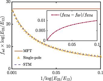
Figure 3. The reduced scattering amplitude $f_\textrm{ad} \log(E_{23}/E_{12}) $ as a function of effective interaction strength $1/\log(E_{23}/E_{12})$. In the limit of weak interaction, both MFT and SPA work well owing to the validity of Born approximation. Inset: with increasing interaction, SPA performs satisfactory with a relative error of ${\sim}1\%$ throughout the entire regime under consideration. |
3. Three-body recombination rate
Three-body recombination is a fundamental, and in many cases dominating, loss channel in dilute quantum gases, under which two out of three free particles form a dimer and the third one escapes from the system by taking the binding energy. This process directly affects the lifetime of quantum gases, especially in the intermediate and strong interaction regimes. In this section, we solve the STM equations to obtain the wave function of scattering state and estimate the lifetime of the quantum gas corresponding to the recombination process. As a concrete example, we focus on a system with equal masses $M = 1$. The case of general mass ratio can be analyzed analogously.
Three-body recombination can be studied by considering an inverse process of atom-dimer scattering that ends up with three free particles, as illustrated in the bottom channel of figure 1. For that purpose, we naturally take the energy of a single particle as $\mu = 4\pi \hbar^2 n/ m \require{physics}\abs{\log(n a_\mathrm{2D}^2)}$, and consider an elastic scattering with energy $E = 3\mu$. In the frame of center-of-mass momentum, the three outgoing atoms leave with momenta of the same magnitude $q = \sqrt{2mE/3}$ but different directions, and the outgoing state is described as $\ket{\Psi_\mathrm{out}} = \ket{\boldsymbol{k}_0}_{23} \ket{\boldsymbol{K}_f}_{1{\textrm{-}}23} $ in relative momentum representation with $k_0 = \sqrt{3}q/2$ and $K_f = q$.
The interactions between particles are described as in equation (3 ) with $g_{ij} = g_\mathrm{2D}$ and $E_{ij} = E_{b}$. Since the masses are the same, the operators of relative momentum can be simplified as $ \boldsymbol{k}_{12} = ({1}/{2}) (\boldsymbol{k}_1 -\boldsymbol{k}_2)$, $\boldsymbol{K}_{3{\textrm{-}}12} = ({1}/{3}) [ - (\boldsymbol{k}_{1}+\boldsymbol{k}_{2}) + 2\boldsymbol{k}_3 ]$, and $\boldsymbol{K}_\textrm{tot} = \boldsymbol{k}_1 +\boldsymbol{k}_2 +\boldsymbol{k}_3$. For the case of a zero total momentum, we reach the cyclically symmetric form of free Hamiltonian $H_0 = \boldsymbol{k}_{ij}^2 + 3 \boldsymbol{K}_{k{\textrm{-}}ij}/4$ and the corresponding free Green’s function
$\begin{align} G_{0} = \int\mathrm{d}\boldsymbol{k}\mathrm{d}\boldsymbol{K} \frac{\ket{\boldsymbol{k}}_{ij} \bra{\boldsymbol{k}} \otimes \ket{\boldsymbol{K}}_{k{\textrm{-}}ij} \bra{\boldsymbol{K}}}{E +\textrm{i}\varepsilon -k^2 -3K^2/4} ,\end{align}$
where $(ijk)$ is selected from permutations of $(123)$. For a general three-body process with non-zero incoming momentum $\boldsymbol{K_0}$, the initial state reads $\ket{\Psi_{\boldsymbol{K}_0}^\mathrm{in}} = \ket{\phi_b}_{12} \ket{\boldsymbol{K}_0}_{3{\textrm{-}}12}$ and the scattering energy $E = {3}K_0^2/4 - E_{b} $ with $E_b = 1/a_\mathrm{2D}^2$.By multiplying $(2\pi/g_\mathrm{2D}) {}_{3{\textrm{-}}12} \bra{\boldsymbol{K}} _{12} \bra*{\boldsymbol{k}} V_{12}$ on both sides of the LS equation (2 ), we obtain 6 )–(9 ) and constructing similar auxiliary functions as in equation (8 ), we find that the terms involving $\delta(\boldsymbol{K} - \boldsymbol{K}_0)$ vanish on both sides of equation (25 ), leading to the first STM equation
$\begin{align} \frac{1}{g_\mathrm{2D}}\eta\left(\boldsymbol{K}\right) & = 2 \int \frac{\mathrm{d}\boldsymbol{K}^{^{\prime}}}{\left(2\pi\right)^2} \frac{\chi\left(\boldsymbol{K^{^{\prime}}}\right)}{E + \textrm{i}\varepsilon - K^{^{\prime} 2} - K^2 - \boldsymbol{K \cdot K^{^{\prime}}}} \nonumber\\ &\quad + \textrm{i}\varepsilon \delta\left(\boldsymbol{K - K_0 }\right) \int \frac{\mathrm{d}\boldsymbol{k}}{2\pi} \frac{\phi_b\left(k\right)}{E+\textrm{i}\varepsilon-k^2 - \frac{3}{4} K_0^2} \nonumber \\ &\quad+ \int \frac{\mathrm{d}\boldsymbol{k}}{\left(2\pi\right)^2} \frac{\eta\left(\boldsymbol{K}\right)} {E+\textrm{i}\varepsilon-k^2 - \frac{3}{4}K^2}.\end{align}$
Here, the 2D interaction strength $g_\mathrm{2D}$ satisfies the renormalization relation $1/g_\mathrm{2D} = - (2\pi)^{-2} \int \mathrm{d}\boldsymbol{k} (k^2 + E_b)^{-1} $, and the bound state wave function reads $\phi_b(\boldsymbol{k}) = {\sqrt{E_b/\pi}}/({k^2+ E_b})$. With that, we replace the bare interaction strength with functions of binding energy $E_{b}$ and have $\begin{align} & \frac{1}{4\pi} \log\left({\frac{E_b}{\frac{3}{4} K^2 - E -\textrm{i}\varepsilon}}\right) \eta\left(\boldsymbol{K}\right) + \frac{\textrm{i}\varepsilon }{2 \sqrt{\pi E_b } } \delta\left(\boldsymbol{K} - \boldsymbol{K_0}\right)\nonumber\\ &\quad = 2\int \frac{\mathrm{d}\boldsymbol{K}^{^{\prime}}}{\left(2\pi\right)^2} \frac{\chi\left(\boldsymbol{K^{^{\prime}}}\right)}{E +\textrm{i}\varepsilon -K^{^{\prime} 2} - K^2-\boldsymbol{K \cdot K^{^{\prime}}}}.\end{align}$
Following the same procedure as in equations ( $\begin{align} \log{\frac{E_b}{\frac{3}{4}K^2 - E -\textrm{i}\varepsilon}} \frac{f\left(\boldsymbol{K}\right)}{K^2} = \int \frac{\mathrm{d}\boldsymbol{K}^{^{\prime}}}{\pi} \frac{2\zeta\left(\boldsymbol{K}^{^{\prime}}\right)} {K^{^{\prime} 2} + K^2+\boldsymbol{K \cdot K^{^{\prime}}} - E -\textrm{i}\varepsilon}.\end{align}$
For the second STM equation, we multiply $(2\pi/g_\mathrm{2D}) {}_{2{\textrm{-}}31}\bra{\boldsymbol{K}} {}_{31}$ $\bra*{\boldsymbol{k}} V_{31}$ on the LS equation and obtain $\begin{align} & \log{\frac{E_b} {\frac{3}{4} K^2 -E -\textrm{i}\varepsilon}} \zeta\left(\boldsymbol{K}\right) + \int \frac{\mathrm{d}\boldsymbol{K}^{^{\prime}}}{\pi}\frac{\zeta\left(\boldsymbol{K}^{^{\prime}}\right) - f\left(\boldsymbol{K}^{^{\prime}}\right)/K^{^{\prime} 2}}{K^{^{\prime} 2} + K^2 + \boldsymbol{K \cdot K^{^{\prime}}} -E -\textrm{i}\varepsilon} \nonumber \\ & \quad + \frac{4\pi}{K^2 + \boldsymbol{K}_0 \cdot \boldsymbol{K} + K_0^2 -E -\textrm{i}\varepsilon} = 0.\end{align}$
We emphasize that in the case of a finite incident momentum, the functions $f$ and $\zeta$ both carry an index $\boldsymbol{K}_0$, indicating that in principle they depend on both the norm and direction of incident momentum. However, since only the quantity $\zeta_{\boldsymbol{K}_0}(K = K_f )$ is required in the scattering $T$-matrix, the physics therein should be independent of the direction of $\boldsymbol{K}_0$, and affected by the magnitude $K_0 = |\boldsymbol{K_0}|$ only. Thus, we formally define the angle-average of $f$ and $\zeta$, denoted by $\bar{f}$ and $\bar{\zeta}$ respectively, as
$\begin{align} \bar{f} &\equiv \frac{1}{2\pi} \int \mathrm{d}\theta f_{\boldsymbol{K_0} = \left(K_0,\theta\right)}, \nonumber \\ \bar{\zeta} &\equiv \frac{1}{2\pi} \frac{K_0 - K}{K_0 - K_f} \int \mathrm{d}\theta \zeta_{\boldsymbol{K_0} = \left(K_0,\theta\right)},\end{align}$
satisfying $\bar{f}(K_f) = f (\boldsymbol{K}_f)$, $\bar{\zeta}(K_f) = \zeta(\boldsymbol{K}_f)$ and $K_f = \sqrt{2mE/3}$. Here, we remove the pole of $\zeta$ at $K = K_0$ by including a factor $(K_0 - K)/(K_0 - K_f)$ in the definition of $\bar{\zeta}$. The functions $\bar{f}$ and $\bar{\zeta}$ then become isotropic, such that we can integrate out the angular term and obtain $\begin{align} &\log{\frac{E_b }{\frac{3}{4} K^2 -\textrm{i}\varepsilon - E }} \frac{\bar{f}_{K_0}\left(K\right)}{K^2} - \int K^{^{\prime}}\mathrm{d} K^{^{\prime}} \frac{4\bar{\zeta}_{K_0}\left(K^{^{\prime}}\right) }{\sqrt{\left(K^2 + K^{^{\prime} 2} - E \right)^2 - K^2 K^{^{\prime} 2}} } \frac{K_0 - K_f }{K_0- K^{^{\prime}}} = 0 , \nonumber \\ & \log{\frac{E_b} {\frac{3}{4} K^2 -\textrm{i}\varepsilon - E}} \frac{K_0 - K_f}{K_0 - K} \bar{\zeta}_{K_0} \left(K\right) + 2 \int K^{^{\prime}} \mathrm{d} K^{^{\prime}} \frac{\bar{\zeta}_{K_0} \left(K^{^{\prime}}\right) \left(K_0 - K_f \right) / \left(K_0 - K^{^{\prime}}\right) - \bar{f}_{K_0} \left(K^{^{\prime}}\right)/K^{^{\prime} 2}}{\sqrt{\left(K^2 + K^{^{\prime} 2} - E \right)^2 - K^2 K^{^{\prime} 2}} } \nonumber\\ &\quad + \frac{4\pi}{\sqrt{\left(K^2 + K_0^2 - E \right)^2 - K^2 K_0^2}} = 0.\end{align}$
By solving the equations numerically, we obtain the wave function $\zeta$ in terms of the parameter $t \equiv \arctan(K)$, as displayed in figure 4 for a dimensionless binding energy $n E_b = 1000$. The function $\zeta$ can be directly connected to the lifetime of a quantum gas via the scattering $T$-matrix, with incoming state $\ket{\Psi_\mathrm{in}} = \ket{\phi_b}_{12} \ket{\boldsymbol{K}_0}_{3{\textrm{-}}12} $ and outgoing state $\ket{\Psi_\mathrm{out}} = \ket{\boldsymbol{k}_0}_{23} \ket{\boldsymbol{K}_f}_{1{\textrm{-}}23} $. By defining $\ket{\Psi_+}$ as the scattering state, we consider the cyclical permutations of the total three channels from bound states (12 ), (23 ) and (31 ) to $\ket{\Psi_\mathrm{out}}$, and write down the $T$-matrix as
$\begin{align} t_{if} = 3 \bra{\Psi_\mathrm{out}} \left( V_{23} + V_{31} \right) \ket{\Psi_+} = -\frac{3\sqrt{E_b}}{2 \pi^{5/2} } \bar{\zeta}\left({K = K_f}\right).\end{align}$
The lifetime of the quantum gas is approximated as $\begin{align} \tau\left(x\right) \approx \frac{m a_\mathrm{2D}^2}{3\hbar x^2 F\left(x\right)},\end{align}$
with $F(x) = {(m^2 t_{if}^2)}/{(3\hbar^2 a_\mathrm{2D})^2}$ and the gas parameter $x = n a_\mathrm{2D}^2$. Upon setting $n = 1$, we find the quantity corresponding to $1/x^2F(x)$ is approximated by $4\pi^5/\zeta^2$. The lifetime due to the three-body recombination is displayed in figure 5. As can be expected, the lifetime decreases with the 2D gas parameter $n a_\textrm{2D}^2$. The dependence is nearly a power law with an exponent ${\sim}{-}2.45$.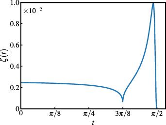
Figure 4. The scattering wave function $\zeta $. We parameterize the STM equations by setting $t = \arctan K \in (0, {\pi}/{2}) $, and transform the integrals in equation ( |
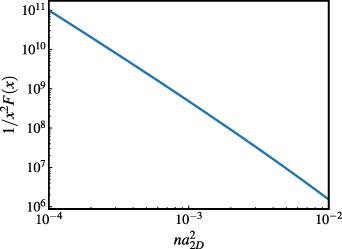
Figure 5. The dimensionless quantity $1/x^2 F(x)$ varying with 2D gas parameter $x = n a_\mathrm{2D}^2$. This quantity is linked to the gas lifetime with $\tau \approx {m a_\mathrm{2D}^2}/{3\hbar x^2 F(x)} $. The dependence is nearly a power law with the exponent ${\sim}{-}2.45$. |
4. Conclusion
In summary, we have theoretically investigated the atom-dimer scattering and three-body recombination processes in 2D ultracold quantum gases using the exact STM equations. For the atom-dimer scattering process, we demonstrated that in the weakly interacting limit, both the MFT and SPA naturally converge to the exact STM solutions. However, as the dimensionless interaction strength increases, the MFT rapidly deviates from the exact result. In stark contrast, the SPA maintains a remarkably high accuracy (with a relative error of ${\sim}1\% $) across a broad interaction regime. This observation indicates that mild intra-species coupling contributes minimally to the rearrangement of the dimer during scattering, highlighting a qualitative difference between 2D and 3D few-body physics. Furthermore, by generalizing the STM equations to accommodate non-zero initial relative momenta, we calculated the exact scattering wave functions to evaluate the three-body recombination rate. Our analysis provides a quantitative estimation for the collisional lifetime of the quantum gas. We found that the gas lifetime is strongly suppressed by enhanced interactions and exhibits a nearly power-law decay with respect to the 2D gas parameter $na_\textrm{2D}^2$, characterized by an exponent of approximately $-2.45$. Our findings clarify the validity boundaries of standard theoretical approximations in reduced dimensions and establish a robust theoretical benchmark for predicting the collisional stability of multicomponent cold atomic mixtures. Looking forward, the methodology presented in this work can be extended to explore more complex few-body scenarios, such as higher-partial-wave (e.g. $p$-wave) interactions, thereby further enriching our understanding of universal few-body physics in low-dimensional quantum systems.
Appendix A. Wave function of the 2D bound state
We start from the fact that the 2D bound state in real space $\phi_b(\boldsymbol{r}) \propto K_0 (\kappa \boldsymbol{r})$ with $\kappa = \sqrt{{2m E_b}/{\hbar^2}}$. The normalization coefficient is obtained by
$\begin{align} \int \mathrm{d}\boldsymbol{r} |K_0\left(\kappa \boldsymbol{r}\right)|^2 = \frac{\pi}{\kappa^2} \Rightarrow \phi_b\left(\boldsymbol{r}\right) = \sqrt{\frac{E_b}{\pi}} K_0 \left(\kappa \boldsymbol{r}\right) ,\end{align}$
where we set $\hbar = 1$ and the reduced mass $m = {1}/{2}$. The Fourier transformation is then applied $\begin{align} \phi_b\left(k\right) = \frac{1}{2\pi} \int \mathrm{d}\boldsymbol{r}\, \sqrt{\frac{E_b}{\pi}} \textrm{e}^{-\textrm{i}\boldsymbol{k}\cdot\boldsymbol{r}} K_0\!\left(\kappa r\right) = \sqrt{\frac{E_b}{\pi}} \frac{1}{k^2 + E_b},\end{align}$
where in the last step we use the fact that $\int\mathrm{d} r \ r K_{0}(k_1 r) J_0(k_2 r) = {1}/{(k_1^2 + k_2^2)} $.Appendix B. Auxiliary function $f(\boldsymbol{K})$ and connection to scattering amplitude
In the section, we first present the LS equation describing two-body scattering, and derive the exact form of 2D scattering amplitude for a general interatomic interaction. Then, we consider contact interaction and solve the three-body scattering problem to obtain the atom-dimer scattering amplitude $f_\mathrm{ad}$. We also prove the auxiliary function $f(\boldsymbol{K})$ defined by equation (8 ) satisfies the limiting condition $\lim_{\varepsilon \to 0^+} f(\boldsymbol{K}) \require{physics}|_{\boldsymbol{K} = 0} = f_\mathrm{ad}$.
B.1. Definition of scattering amplitude
The scattering amplitude in two dimensions is defined by the asymptotic behavior of the scattering state wave function via
$\begin{align} \psi_+\left(\boldsymbol{r}\right) \xrightarrow{kr \to +\infty} \frac{1}{2\pi} \left( \textrm{e}^{\textrm{i} \boldsymbol{k} \cdot \boldsymbol{r}} - f_\textrm{2D} \sqrt{\frac{\textrm{i}}{8 \pi k r} } \textrm{e}^{\textrm{i}kr} \right) .\end{align}$
To derive the exact form of scattering amplitude, we start from the LS equation $\ket{\psi_+} = \ket{\psi_\mathrm{in}} + G_0 V \ket{\psi_+}$ of a two-body scattering problem, where the two-body Green’s function is defined as $G_0 = (E+\textrm{i}\varepsilon - H_0)^{-1}$. By substituting the coordinate representation $G_0(\boldsymbol{r},\boldsymbol{r^{^{\prime}}}) = - {m} K_0 (-\textrm{i}k|\boldsymbol{r}-\boldsymbol{r^{^{\prime}}}|) / {\pi\hbar^2}$ and setting $\hbar = 1$, the wave function of scattering state reads $\begin{align} \psi_+\left(\boldsymbol{r}\right) = \frac{\textrm{e}^{\textrm{i} \boldsymbol{k}\cdot \boldsymbol{r}}}{2\pi} - \frac{m}{\pi} \int \mathrm{d}\boldsymbol{r}^{^{\prime}} K_0\left(-\textrm{i}k|\boldsymbol{r^{^{\prime}}} - \boldsymbol{r}|\right) V\left(\boldsymbol{r^{^{\prime}}}\right) \bra{\boldsymbol{r}^{^{\prime}}} \ket{\psi_+}.\end{align}$
We then expand the Green’s function in the asymptotic region $|\boldsymbol{r}-\boldsymbol{r}^{^{\prime}}| \to +\infty$. In this limit, the relative coordinate between atoms $ |\boldsymbol{r} - \boldsymbol{r}^{^{\prime}}| \to r (1-{\boldsymbol{r}\cdot \boldsymbol{r}^{^{\prime}}}/{r^2}) $. The Bessel function is then expanded into series as $K_0(-\textrm{i}x) \to \textrm{e}^{\textrm{i}(x + \pi/4)} \sqrt{{\pi}/{2x}}$. Combining the two expansions above, we have $\begin{align} \psi_+\left(\boldsymbol{r}\right) & \approx \frac{\textrm{e}^{\textrm{i} \boldsymbol{k}\cdot \boldsymbol{r}}}{2\pi} - \frac{m}{\pi} \sqrt{\frac{\pi}{2}} \frac{\textrm{e}^{\textrm{i}\left(kr + \pi/4\right)}}{\sqrt{kr}} \int \mathrm{d}\boldsymbol{r}^{^{\prime}} \bra{k\hat{r}} \ket{\boldsymbol{r}^{^{\prime}}} V\left(\boldsymbol{r^{^{\prime}}}\right) \bra{\boldsymbol{r}^{^{\prime}}} \ket{\psi_+} \nonumber\\ & \approx \frac{\textrm{e}^{\textrm{i} \boldsymbol{k} \cdot \boldsymbol{r}}}{2\pi} - m \sqrt{2\pi} \frac{\textrm{e}^{\textrm{i}\left(kr + \pi/4\right)}}{\sqrt{kr}} \bra{\psi_\mathrm{in}} V \ket{\psi_+} ,\end{align}$
where in the second line we have used the approximation that the direction of position vector $\hat{r}$ coincides with the incoming wave vector $\boldsymbol{k}$, together with the selection of initial state $\ket{k\boldsymbol{r}} = \ket{\psi_\mathrm{in}}$. The scattering amplitude is then written as $f_\mathrm{2D} = 2m (2\pi)^2 \bra{\psi_\mathrm{in}} V \ket{\psi_+}$. We generalize the expression to the problem of atom-dimer scattering and have $\begin{align}f_\textrm{ad} = 2m_\textrm{ad} \left(2\pi\right)^2 \bra{\Psi_\mathrm{in}} \left(V_{31} + V_{23}\right) \ket{\Psi_+},\end{align}$
with reduced mass $m_\mathrm{\textrm{ad}} = {2M}/{(M+1)}$ and initial state $\ket{\Psi_\mathrm{in}} = \ket{\phi_\mathrm{b}}_{12} \ket{\boldsymbol{K}_0}_{3{\textrm{-}}12} $.B.2. Expression of $f(\boldsymbol{K})$
To obtain the expression of $f(\boldsymbol{K})$, which is related to the atom-dimer scattering amplitude, we first write the three-body LS equation as B5 ) as 3 ). Considering the action of interaction operators as in equation (4 ), we may apply $_ {3{\textrm{-}}12}\bra{\boldsymbol{K}} {}_{12}\bra{\boldsymbol{k}_0}$ on both sides of equation (B7 ) to reach
$\begin{align} \ket{\Psi_{+}\left(\varepsilon\right)} = \lim_{\varepsilon\rightarrow 0^{+}} \frac{\textrm{i}\varepsilon}{-E_{12} +\textrm{i}\varepsilon -H} \ket{\Psi_{\textrm{in}}},\end{align}$
where the corresponding Hamiltonian reads $H = T + V_{12} + V_{23} + V_{31}$ and $T = k_{12}^2 + \frac{3}{4} K_{3{\textrm{-}}12}^2$. We now separate the Green’s function $G_{3}(\varepsilon) \equiv [-E_{12}+\textrm{i}\varepsilon -(T+V_{23}) ]^{-1} = G^{(0)}_{3}(\varepsilon) +G^{(1)}_{3}(\varepsilon)$, with $\begin{align}G^{\left(0\right)}_{3}\left(\varepsilon\right) & = \int\mathrm{d}\boldsymbol{K} \frac{\ket{\phi_{b}}_{12} \bra{\phi_{b}} \otimes \ket{\boldsymbol{K}}_{3{\textrm{-}}12} \bra{\boldsymbol{K}} }{\textrm{i}\varepsilon-3K^2/4}, \nonumber\\ G^{\left(1\right)}_{3}\left(\varepsilon\right) & = \int \mathrm{d}\boldsymbol{k} \mathrm{d}\boldsymbol{K} \frac{\ket{\boldsymbol{k+}}_{12} \bra{\boldsymbol{k+}} \otimes \ket{\boldsymbol{K}}_{3{\textrm{-}}12} \bra{\boldsymbol{K}}} {-E_{12} +\textrm{i}\varepsilon -k^2-3K^2/4},\end{align}$
where $\ket{\boldsymbol{k}+}_{12}$ denotes the scattering state between atoms 1 and 2. With that, we can rewrite equation ( $\begin{align} \ket{\Psi_{+}\left(\varepsilon\right)} = \ket{\Psi_{\textrm{in}}} + G_{3}\left(\varepsilon\right) \left(V_{23}+V_{31}\right) \ket{\Psi_{+}\left(\varepsilon\right)} ,\end{align}$
and the interaction potential is given in equation ( $\begin{align} \eta\left(\boldsymbol{K}\right) & = g_{12}\ {}_{3{\textrm{-}}12} \bra{\boldsymbol{K}}{}_{12} \bra{\phi}\ket{\Psi_{\textrm{in}}}+ g_{12}\ {}_{3{\textrm{-}}12} \bra{\boldsymbol{K}}{}_{12} \bra{\phi} G_{3}^{\left(0\right)} \nonumber\\ & \quad \times\left(\varepsilon\right) \left( V_{23} + V_{31} \right) \ket{\Psi_{+} \left(\varepsilon\right)} + g_{12}\ {}_{3{\textrm{-}}12} \bra{\boldsymbol{K}}{}_{12} \bra{\phi} G_{3}^{\left(1\right)} \nonumber\\ &\quad \times \left(\varepsilon\right) \left( V_{23} + V_{31} \right) \ket{\Psi_{+} \left(\varepsilon\right)} .\end{align}$
The first term of equation (B8 ) can be simplified as $g_{12}\ {}_{3{\textrm{-}}12} \bra{\boldsymbol{K}} {}_{12}\bra{\phi} \ket{\Psi_{\textrm{in}}} = g_{12} \int {\mathrm{d}\boldsymbol{k}}\phi_b(\boldsymbol{k}) \delta(\boldsymbol{K}) / {2\pi}$$= -2 \sqrt{E_{12} \pi} \delta(\boldsymbol{K})$. Here, we set the initial state with total momentum $\boldsymbol{K}_\mathrm{tot} = \boldsymbol{0}$, and introduce the 2D bound state wave function $\phi_b(\boldsymbol{k}) = \sqrt{{E_{12}}/{\pi}}/ (k^2+E_{23})$ and the 2D renormalization relation. We can impose the renormalization relation analogously and write the second term of equation (B8 ) as
$\begin{align} & g_{12} \int \frac{\mathrm{d}\boldsymbol{k}}{2\pi} \mathrm{d}\boldsymbol{K^{^{\prime}}} \frac{{}_{12}\bra{\boldsymbol{k}} \ket{\phi_{b}}_{12} \bra{\phi_{b}} \otimes {}_{3{\textrm{-}}12} \bra{\boldsymbol{K}} \ket{\boldsymbol{K^{^{\prime}}}}_{3{\textrm{-}}12}\bra{\boldsymbol{K^{^{\prime}}}}} {\textrm{i}\varepsilon-3K^{^{\prime} 2}/4} \left(V_{23} + V_{31}\right) \ket{\Psi_{+} \left(\varepsilon\right)} \nonumber\\ &\quad = -\frac{2 \sqrt{E_{12} \pi}}{\textrm{i}\varepsilon-3K^2/4} {}_{3{\textrm{-}}12} \bra{\boldsymbol{K}}{}_{12} \bra{\phi_{b}} \left(V_{23} + V_{31}\right) \ket{\Psi_{+} \left(\varepsilon\right)},\end{align}$
and the third term as $\begin{align} g_{12} \int \frac{\mathrm{d}\boldsymbol{k}}{2\pi}\mathrm{d}\boldsymbol{k^{^{\prime}}} \frac{ {}_{12} \bra{\boldsymbol{k}} \ket{\boldsymbol{k^{^{\prime}}+}}_{12} \bra{\boldsymbol{k^{^{\prime}}+}} {}_{3{\textrm{-}}12} \bra{\boldsymbol{K}}} {-E_{12} + \textrm{i}\varepsilon -k^{^{\prime} 2} -3K^2/4} \left(V_{23} + V_{31}\right) \ket{\Psi_{+} \left(\varepsilon\right)}.\end{align}$
Next, we consider a contact interaction with B12 ) then reduces to B10 ) as
$\begin{equation} \bra{\boldsymbol{r}} \ket{\boldsymbol{k}+} = \frac{1}{2\pi} \left[ \textrm{e}^{\textrm{i}\boldsymbol{k}^{^{\prime}}\cdot\boldsymbol{r}} + \frac{K_0\left(-\textrm{i}k^{^{\prime}}r\right)}{\log\left(\frac{k^{^{\prime}}a_\textrm{2D} }{2\textrm{i}}\right) + \gamma} \right],\end{equation}$
with $a_\mathrm{2D}$ and $\gamma$ the 2D scattering amplitude and Euler-constant, respectively. The inner product of scattering state $\ket{\boldsymbol{k}^{^{\prime}}+}$ and momentum eigenstate $\ket{\boldsymbol{k}}$ reads $\begin{align} {}_{12}\bra{\boldsymbol{k}} \ket{\boldsymbol{k}^{^{\prime}}+}_{12} = \delta\left(\boldsymbol{k}-\boldsymbol{k}^{^{\prime}}\right) + \frac{1}{2\pi} \int r\mathrm{d}{r} J_0\left(kr\right) \frac{K_0\left(-\textrm{i}k^{^{\prime}}r\right)}{\log\left(\frac{k^{^{\prime}} a_\textrm{2D}}{2\textrm{i}}\right) + \gamma},\end{align}$
where we used the identity $J_0(x) = ({1}/{2\pi}) \int_{0}^{2\pi} \textrm{e}^{\textrm{i}x \cos\theta}$. To integrate out the coordinate $r$, we use the integral formula $\begin{align} \int_{0}^{a} x J_\nu\left(\lambda x\right) K_\nu\left(\mu x\right) \mathrm{d}{x} & = \frac{1}{\mu^2+\lambda^2} \Big[ \left( \frac{\lambda}{\mu} \right)^\nu + \lambda a J_{\nu+1}\left(\lambda a\right) K_\nu\left(\mu a\right) \nonumber\\ &\quad - \mu a J_\nu\left(\lambda a\right) K_{\nu+1}\left(\mu a\right) \Big],\end{align}$
with parameters $\nu = 0$, $\lambda = k$ and $\mu = -\textrm{i}k^{^{\prime}}$. The integral then becomes $\begin{align} &\int_{0}^{+\infty} r\mathrm{d}{r}\, J_0\left(kr\right) K_0\left(-\textrm{i}k^{^{\prime}}r\right) = \frac{1}{k^2-k^{^{\prime} 2}} + \frac{1}{k^2-k^{^{\prime} 2}}\nonumber\\&\quad \times \lim_{a\to+\infty} a \left[ k J_1\left(ka\right) K_0\left(-\textrm{i}k^{^{\prime}}a\right)+ \textrm{i}k^{^{\prime}} J_0\left(ka\right) K_1\left(-\textrm{i}k^{^{\prime}}a\right) \right].\end{align}$
The asymptotic behavior of integral as $a \to +\infty$ can be obtained by writing the Bessel functions as $\begin{align} &J_0\left(x\right) \to \sin \left( x + \frac{\pi}{4} \right) \sqrt{\frac{2}{\pi x}} , \qquad J_1\left(x\right) \ \to -\cos \left( x+\frac{\pi}{4} \right) \sqrt{\frac{2}{\pi x}} , \nonumber\\ & K_0\left(-\textrm{i}x\right) \to \textrm{e}^{\textrm{i}x} \sqrt{\frac{\pi}{2}} \frac{1}{\sqrt{-\textrm{i}x}} , \qquad \ K_1\left(-\textrm{i}x\right) \to \textrm{e}^{\textrm{i}x} \sqrt{\frac{\pi}{2}} \frac{1}{\sqrt{-\textrm{i}x}}, \nonumber \\ \end{align}$
and using the convention of the arguments $\textrm{i} = \textrm{e}^{\textrm{i}{\pi}/{2}}$ and ${1}/{\sqrt{-\textrm{i}}} = \textrm{e}^{\textrm{i}{\pi}/{4}}$. The inner product between momentum state and scattering state in equation ( $\begin{align}{}_{12}\bra{\boldsymbol{k}}\ket{\boldsymbol{k}^{^{\prime}}+}_{12} & = \delta\left(\boldsymbol{k}-\boldsymbol{k}^{^{\prime}}\right) + \frac{1}{2\pi} \Bigg\{\frac{1}{k^2-k^{^{\prime} 2}} + \frac{1}{2 \sqrt{kk^{^{\prime}}}}\nonumber\\ &\quad \times \lim_{a\to+\infty} \left[ \frac{\textrm{i} \textrm{e}^{\textrm{i} \left(k+k\right)a }}{k^{^{\prime}} + k} - \frac{\textrm{e}^{-\textrm{i} \left(k^{^{\prime}}+k\right) a }}{k^{^{\prime}}+k} \right] \Bigg\} \frac{1}{\log\left(\frac{k^{^{\prime}} a_{2D}}{2\textrm{i}}\right) + \gamma} .\end{align}$
With that, we can rewrite equation ( $\begin{align} & \frac{g_{12}}{2\pi} \int \mathrm{d}{\boldsymbol{k}} \frac{{}_{12} \bra{\boldsymbol{k}+} {}_{3{\textrm{-}}12}\bra{\boldsymbol{K}} \left(V_{23}+V_{31}\right)\ket{\Psi_+}} {-E_{12} + \textrm{i}\varepsilon - k^2 - \frac{3}{4}K^2} \nonumber\\ &\quad+ \frac{g_{12}}{\left(2\pi\right)^2} \int_0^{+\infty} k\mathrm{d}{k}\mathrm{d}{\boldsymbol{k}^{^{\prime}}} \Bigg\{\frac{1}{k^2-k^{^{\prime} 2}} + \frac{1}{2\sqrt{kk^{^{\prime}}}} \nonumber\\ &\quad\times \lim_{a\to+\infty} \left[ \frac{\textrm{i} \textrm{e}^{\textrm{i}\left(k^{^{\prime}}+k\right)a}}{k^{^{\prime}}+k} - \frac{\textrm{e}^{\textrm{i}\left(k^{^{\prime}}-k\right)a}}{k^{^{\prime}}-k} \right] \Bigg\} \nonumber\\ &\quad \times \frac{1}{\log\left(\frac{k^{^{\prime}} a_\textrm{2D}}{2\textrm{i}}\right)+\gamma} \frac{{}_{12} \bra{\boldsymbol{k}^{^{\prime}}+} {}_{3{\textrm{-}}12} \bra{\boldsymbol{K}} \left(V_{23}+V_{31}\right) \ket{\Psi_+}} {-E_{12} + \textrm{i}\varepsilon - k^{^{\prime} 2} - \frac{3}{4} K^2}.\end{align}$
Next, we focus on the second line of the equation above B18 ) as B10 ) as B8 ) can be reformed as
$\begin{align} \frac{g_{12}}{\left(2\pi\right)^2} \int_0^{+\infty} k\mathrm{d}{k} \left\{\frac{1}{k^2-k^{^{\prime} 2}} + \frac{1}{2\sqrt{kk^{^{\prime}}}} \lim_{a\to+\infty} \left[ \frac{\mathrm{i} \textrm{e}^{\textrm{i}\left(k^{^{\prime}}+k\right)a}}{k^{^{\prime}}+k} - \frac{\textrm{e}^{\textrm{i}\left(k^{^{\prime}}-k\right)a}}{k^{^{\prime}}-k} \right] \right\}.\end{align}$
The term involving $1/(k^2-k^{^{\prime} 2})$ can be evaluated directly by applying the renormalization relation with a momentum cutoff $\Lambda$, followed by taking the limit $\lim_{\Lambda\to+\infty}$, leading to $\begin{align} \frac{g_{12}}{\left(2\pi\right)^2} \int_0^{+\infty} k\mathrm{d}{k} \frac{1}{k^2-k^{^{\prime} 2}} = -\lim_{\Lambda\to+\infty} \frac{\frac{1}{2} \log\left(\frac{\Lambda^2 - k^{^{\prime} 2}}{k^{^{\prime} 2}}\right) }{\pi \log\left(\frac{\Lambda^2 + E_{12}}{E_{12}}\right)} = - \frac{1}{2\pi}.\end{align}$
The integral involving the $1/\sqrt{kk^{^{\prime}}}$ term can be recast into $\begin{align} \frac{g_{12}}{\left(2\pi\right)^2} \int_{-\infty}^{+\infty} \mathrm{d}{k} \frac{\sqrt{k}}{2\sqrt{k^{^{\prime}}}} \lim_{a\to+\infty} \frac{\textrm{e}^{\textrm{i}\left(k^{^{\prime}}-k\right)a}}{k-k^{^{\prime}}}.\end{align}$
We now assume that the integrals are understood as the principal integrals, and are uniformly convergent to allow for an interchange of integral and limit. Then we construct the following integral of complex variable functions $\begin{align} \mathrm{Int} \equiv \int_{z = -\infty}^{+\infty} \mathrm{d} z \ \frac{z^{1/2}}{z-z_0} \textrm{e}^{\textrm{i}\left(z-z_0\right)}.\end{align}$
Since the function possesses a single pole at $z = z_0$, we choose the integration contour as illustrated in figure 6, containing one semicircle $C_1$ with $|z|\to +\infty$ in the upper half-plane and one semicircle $c_2$ near the pole in the upper half-plane. By using Cauchy’s theorem, and the fact that $\int_{C_1} \mathrm{d} z \ \frac{z^{1/2}}{z-z_0} \textrm{e}^{\textrm{i}(z-z_0)} = 0$ and $\int_{c_2} \mathrm{d} z \ \frac{z^{1/2}}{z-z_0} \textrm{e}^{\textrm{i}(z-z_0)} = - \pi \textrm{i}$, we can calculate the second term of equation ( $\begin{align} & \frac{g_{12}}{\left(2\pi\right)^2} \int_0^{+\infty} \mathrm{d}{k} \frac{\sqrt{k}}{2\sqrt{k^{^{\prime}}}} \lim_{a\to+\infty} \left[ \frac{\textrm{i} \textrm{e}^{\textrm{i}\left(k^{^{\prime}}+k\right)a}}{k^{^{\prime}}+k} + \frac{\textrm{e}^{\textrm{i}\left(k^{^{\prime}}-k\right)a}}{k-k^{^{\prime}}} \right]\nonumber\\ &\quad = \lim_{a\to+\infty} \frac{g_{12}}{\left(2\pi\right)^2} \frac{1}{2\sqrt{k^{^{\prime}}a}} \pi \textrm{i} = 0 .\end{align}$
Thus far, we can rewrite equation ( $\begin{align} \frac{1}{2\pi} \int \mathrm{d}{\boldsymbol{k}} \left[ g_{12} - \frac{1}{\log\left(\frac{k a_\textrm{2D}}{2\textrm{i}}\right)+\gamma}\right] \frac{{}_{12} \bra{\boldsymbol{k}+} {}_{3{\textrm{-}}12} \bra{\boldsymbol{K}} \left(V_{23}+V_{31}\right) \ket{\Psi_+}} {-E_{12} + \textrm{i}\varepsilon - k^2 - \frac{3}{4} K^2}.\end{align}$
It is straightforward to conclude that this term vanishes by multiplying $\lim_{\varepsilon\to 0} \left( 4 \mathrm{i} \varepsilon/3 - K^2 \right)\require{physics}|_{K = 0}$. Then, equation ( $\begin{align} \eta\left(\boldsymbol{K}\right) & = -2 \sqrt{E_{12} \pi } \delta\left(\boldsymbol{K}\right)- \frac{2 \sqrt{E_{12} \pi }} {\textrm{i}\varepsilon-3K^2/4} {}_{3{\textrm{-}}12} \bra{\boldsymbol{K}}{}_{12} \bra{\phi_{b}} \left(V_{23}+V_{31}\right) \ket{\Psi_{+}\left(\varepsilon\right)} \nonumber \\ & \quad + \frac{1}{2\pi} \int \mathrm{d}{\boldsymbol{k}} \left[ g_{12} - \frac{1}{\log\left(\frac{k a_\textrm{2D}}{2\textrm{i}}\right)+\gamma}\right] \frac{{}_{12} \bra{\boldsymbol{k}+} {}_{3{\textrm{-}}12} \bra{\boldsymbol{K}} \left(V_{23}+V_{31}\right) \ket{\Psi_+}} {-E_{12} + \textrm{i}\varepsilon - k^2 - \frac{3}{4} K^2}.\end{align}$
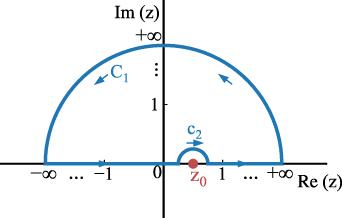


Figure 6. The contour for the complex-variable integral in equation ( |
To obtain the atom-dimer scattering amplitude $f_\mathrm{ad}$, we define the function $f(\boldsymbol{K})$ via equation (8 ). By substituting this definition into equation (B24 ) and multiplying $(\textrm{i}\varepsilon-3K^2/4)$ on both sides, we have
$\begin{align} \frac{1}{\left(2\pi\right)^2} \frac{3f\left(\boldsymbol{K}\right)}{4} & = {}_{3{\textrm{-}}12} \bra{\boldsymbol{K}}{}_{12} \bra{\phi_{b}} \left(V_{23}+V_{31}\right) \ket{\Psi_{+}\left(\varepsilon\right)} \nonumber \\ &\quad - \frac{\textrm{i}\varepsilon -3K^2/4}{4\pi \sqrt{E_{12} \pi}} \int \mathrm{d}{\boldsymbol{k}} \left[ g_{12} - \frac{1}{\log\left(\frac{k a_\textrm{2D}}{2\textrm{i}}\right)+\gamma}\right]\nonumber\\ &\quad \times \frac{{}_{12} \bra{\boldsymbol{k}+} {}_{3{\textrm{-}}12} \bra{\boldsymbol{K}} \left(V_{23}+V_{31}\right) \ket{\Psi_+}} {-E_{12} + \textrm{i}\varepsilon - k^2 - \frac{3}{4} K^2}.\end{align}$
Notice that the terms involving $\delta$ functions are canceled out. In the limit of $\varepsilon\rightarrow 0$ and setting $\boldsymbol{K} = 0$, the last term vanishes and we obtain $\begin{align} \lim_{\varepsilon \to0} f\left(K = 0,\varepsilon\right) = \frac{4M}{M+2} \left(2\pi\right)^2 \bra{\Psi_{\mathrm{in}}} \left(V_{12}+V_{31}\right) \ket{\Psi_{+}\left(\varepsilon\right)},\end{align}$
which is the scattering amplitude by definition.Appendix C. Basis transformation
The basis transformation is derived with the assumption C1 ), we have
$\begin{align} \ket{\boldsymbol{K}}_{1{\textrm{-}}23} \ket{\boldsymbol{k}}_{23} = \ket{a\boldsymbol{k} + b\boldsymbol{K}}_{3{\textrm{-}}12} \ket{c\boldsymbol{k} + d\boldsymbol{K}}_{12}.\end{align}$
The transformation of observable operators are $\begin{align} \hat{{\boldsymbol{K}}}_{3{\textrm{-}}12} = -\hat{{\boldsymbol{k}}}_{23} - \frac{M}{M+1}\,\hat{{\boldsymbol{K}}}_{1{\textrm{-}}23}.\end{align}$
Apply the operators on the corresponding sides of vectors equation ( $\begin{align} \hat{{\boldsymbol{K}}}_{3{\textrm{-}}12} \ket{\boldsymbol{K}}_{1{\textrm{-}}23} \ket{\boldsymbol{k}}_{23} & = \left(-\hat{{\boldsymbol{k}}}_{23} - \frac{M}{M+1}\,\hat{{\boldsymbol{K}}}_{1{\textrm{-}}23}\right) \ket{\boldsymbol{K}}_{1{\textrm{-}}23} \ket{\boldsymbol{k}}_{23}\nonumber\\& = \left( -\boldsymbol{k} - \frac{M}{M+1} \boldsymbol{K} \right) \ket{\boldsymbol{K}}_{1{\textrm{-}}23} \ket{\boldsymbol{k}}_{23},\end{align}$
and $\begin{align} \hat{{\boldsymbol{K}}}_{3{\textrm{-}}12} \ket{a\boldsymbol{k} + b\boldsymbol{K}}_{3{\textrm{-}}12} \ket{c\boldsymbol{k} + d\boldsymbol{K}}_{12} & = \left(a\boldsymbol{k} + b\boldsymbol{K}\right) \ket{a\boldsymbol{k} + b\boldsymbol{K}}_{3{\textrm{-}}12} \ket{c\boldsymbol{k} + d\boldsymbol{K}}_{12}.\end{align}$
By matching the coefficients, we obtain $\begin{align} \ket{\boldsymbol{K}}_{1{\textrm{-}}23} \ket{\boldsymbol{k}}_{23} & = \ket{-\boldsymbol{k} -\frac{M}{M+1}\boldsymbol{K}}_{3{\textrm{-}}12} \ket{-\frac{1}{2}\boldsymbol{k} +\frac{M+2}{2\left(M+1\right)}\boldsymbol{K}}_{12}, \nonumber\\ \ket{\boldsymbol{K}}_{2{\textrm{-}}31} \ket{\boldsymbol{k}}_{31} & = \ket{\boldsymbol{k} -\frac{M}{M+1}\boldsymbol{K}}_{3{\textrm{-}}12} \ket{-\frac{1}{2}\boldsymbol{k} -\frac{M+2}{2\left(M+1\right)}\boldsymbol{K}}_{12}.\end{align}$
Now we consider the interaction potential taking the form as $\begin{align}V_{23}& = \frac{g_{\textrm{23}}}{\left(2\pi\right)^2} \int\mathrm{d}\boldsymbol{k} \mathrm{d}\boldsymbol{k^{^{\prime}}}\mathrm{d}\boldsymbol{K} \left(\ket{\boldsymbol{K}}_{1{\textrm{-}}23} \ket{\boldsymbol{k}}_{23} \right) \otimes \left(\ _{23}\bra{\boldsymbol{k^{^{\prime}}}}_{1{\textrm{-}}23} \bra{\boldsymbol{K}}\right), \nonumber\\ V_{31}& = \frac{g_{23}}{\left(2\pi\right)^2} \int\mathrm{d}\boldsymbol{k} \mathrm{d}\boldsymbol{k^{^{\prime}}}\mathrm{d}\boldsymbol{K} \left(\ket{\boldsymbol{K}}_{2{\textrm{-}}31} \ket{\boldsymbol{k}}_{31}\right) \otimes \left(\ _{31}\bra{\boldsymbol{k^{^{\prime}}}}_{2{\textrm{-}}31} \bra{\boldsymbol{K}}\right),\end{align}$
and directly find the interaction potentials in non-diagonal Jacobi frameworks $\begin{align}V_{31}& = g_{23} \int \mathrm{d}{\boldsymbol{k}} \mathrm{d}{\boldsymbol{k}^{^{\prime}}} \mathrm{d}{\boldsymbol{K}} \left(\ket{\boldsymbol{k}-\frac{M}{M+1} \boldsymbol{K}}_{3{\textrm{-}}12} \ket{-\frac{1}{2}\boldsymbol{k} -\frac{M+2}{2\left(M+1\right)}\boldsymbol{K}}_{12}\right) \nonumber\\ & \quad \otimes \left(_{12} \bra{-\frac{1}{2}\boldsymbol{k}^{^{\prime}} -\frac{M+2}{2\left(M+1\right)}\boldsymbol{K}} _{3{\textrm{-}}12}\bra{\boldsymbol{k}^{^{\prime}} -\frac{M}{M+1}\boldsymbol{K}} \right) , \nonumber\\ V_{23}& = g_{23} \int \mathrm{d}{\boldsymbol{k}} \mathrm{d}{\boldsymbol{k}^{^{\prime}}} \mathrm{d}{\boldsymbol{K}} \left(\ket{-\boldsymbol{k} -\frac{M}{M+1}\boldsymbol{K}}_{3{\textrm{-}}12} \ket{-\frac{1}{2}\boldsymbol{k} +\frac{M+2}{2\left(M+1\right)} \boldsymbol{K}}_{12}\right) \nonumber\\ & \quad \otimes \left(_{12}\bra{-\frac{1}{2}\boldsymbol{k}^{^{\prime}} +\frac{M+2}{2\left(M+1\right)} \boldsymbol{K}} _{3{\textrm{-}}12} \bra{-\boldsymbol{k}^{^{\prime}} -\frac{M}{M+1}\boldsymbol{K}} \right) .\end{align}$