

1. Introduction
The analysis of complex networks has established itself as a unifying paradigm for deciphering systems defined by intricate interactions, spanning biological regulatory circuits, neural connectomes, social hierarchies, and technological infrastructures [1, 2]. A ubiquitous mesoscale feature of such systems is community structure, characterized by the tendency of nodes to organize into groups with dense internal connectivity and comparatively sparse external linkages [3]. Detecting these communities is fundamental to disentangling functional organization, identifying latent modules, and inferring the dynamical processes that govern system behavior.
To rigorously evaluate partition quality, numerous quantitative measures have been developed [4], among which modularity (Q) has emerged as the most influential objective function [5]. Modularity quantifies the deviation of the observed edge density within communities from the expected density in a random null model. However, maximizing modularity is a nondeterministic polynomial-time hard (NP-hard) problem [6]. This intrinsic complexity is highlighted by the development of exact optimization techniques based on integer linear programming, such as the Bayan algorithm [7], which utilize rigorous mathematical proofs to find the global optimum but scale exponentially with system size. Consequently, while exact solvers provide valuable ground truths for small datasets, large-scale network analysis necessitates the use of heuristic approximations.
The landscape of heuristic solvers is rich and varied. Greedy agglomerative algorithms [8] and multi-level refinement strategies, such as the Louvain [9] and Leiden [10] algorithms, strike a practical balance between computational speed and solution quality. Yet, these methods are inherently local in their search dynamics and are notoriously prone to becoming trapped in suboptimal local maxima. Theoretical analyses have shown that the modularity landscape is characterized by extreme degeneracy, containing an exponential number of high-modularity partitions with structurally distinct configurations [11]. Furthermore, modularity optimization is subject to a ‘resolution limit,’ wherein it may fail to resolve small clusters in large networks [12]. These challenges underscore the need for optimization strategies capable of navigating the rugged, glassy energy landscapes where standard heuristics often stall.
A transformative perspective on this challenge is provided by statistical physics, which maps the negative modularity of a partition exactly onto the Energy of a disordered Potts spin glass model [13]. In this isomorphism, nodes correspond to spins, community labels to spin states, and the coupling strengths to the modularity matrix elements. Building on this physical analogy, probabilistic inference methods, most notably the Belief Propagation (BP) algorithm, have been employed to approximate the marginal probabilities of node assignments within the finite-temperature Gibbs distribution [14]. While BP is highly effective for inferring consensus community structures and detecting phase transitions in the detectability of blocks [15], it encounters significant difficulties when used as a ground-state optimizer. In the low-temperature ‘spin-glass phase,’ the free-energy landscape fractures due to replica symmetry breaking [16]. In this regime, message-passing algorithms typically fail to converge to a stable fixed point, oscillating chaotically between metastable states and failing to identify the single partition that maximizes modularity.
To address these optimization deficits, we introduce a solver based on the Free-Energy Machine (FEM) framework [17]. FEM reformulates the discrete combinatorial optimization problem of modularity maximization as a continuous variational inference task. Rather than relying on message passing, this approach minimizes a mean-field approximation to the free energy using gradient-based optimization techniques adapted from machine learning. By integrating an annealing schedule, which gradually transitions the system from a convex high-entropy regime to the ground state with the parallel evolution of multiple independent replicas, FEM effectively traverses the rugged energy landscape. This architecture naturally exploits the massive parallelism of graph processing units (GPUs) to robustly explore the solution space.
In this work, we validate FEM as a high-performance solver for modularity optimization. We compare its performance against state-of-the-art heuristics (Louvain, Leiden), exact solvers (Bayan), and physical algorithms (BP) on a comprehensive suite of benchmarks. These include stochastic block models (SBM) [18], the Lancichinetti–Fortunato–Radicchi (LFR) benchmark [19], and Artificial Benchmark for Community Detection (ABCD) graphs [20], alongside standard real-world networks. Our results demonstrate that FEM consistently identifies partitions with superior modularity, particularly in regimes where the community structure is subtle or the optimization landscape is exceptionally complex.
2. Method
2.1. Modularity as the energy of a Potts model
Community detection in complex networks can be rigorously formulated as a ground-state search problem in statistical physics. The most widely used objective function for quantifying community structure is the modularity Q, introduced by Newman and Girvan [5]. For a network with N nodes and m edges, the modularity of a partition C = {C1, …, CN} is defined as:
$\begin{eqnarray}Q({\boldsymbol{C}})=\frac{1}{2m}\displaystyle \sum _{i,j=1}^{N}\left({A}_{ij}-\frac{{k}_{i}{k}_{j}}{2m}\right)\delta ({C}_{i},{C}_{j}),\end{eqnarray}$
where Aij is the adjacency matrix, ki is the degree of node i, and δ(Ci, Cj) is the Kronecker delta which equals 1 if nodes i and j belong to the same community (Ci = Cj) and 0 otherwise.As established by Reichardt and Bornholdt [13], maximizing equation (1 ) is mathematically equivalent to finding the ground state of an infinite-range Potts model, where the community assignment Ci of q communities is assigned to a q-state Potts spin σi ∈ {1, …, q}. The energy E(σ) of this system is given by:
$\begin{eqnarray}E({\boldsymbol{\sigma }})=-\displaystyle \sum _{i,j=1}^{N}{B}_{ij}\delta ({\sigma }_{i},{\sigma }_{j}),\end{eqnarray}$
where ${B}_{ij}={A}_{ij}-\frac{{k}_{i}{k}_{j}}{2m}$ is the modularity matrix. In this physical picture, Bij represents the coupling strength between spins i and j. The presence of both positive (ferromagnetic) and negative (antiferromagnetic) interactions in Bij induces frustration, creating a spin-glass-like energy landscape with numerous local minima [11]. Consequently, as shown in figure 1, maximizing Q is equivalent to minimizing the spin-glass energy E(σ), and thus finding the global maximum of Q remains an NP-hard combinatorial optimization problem [6].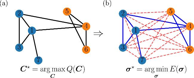
Figure 1. Mapping between community detection and spin glass systems. (a) Illustration of community detection, where nodes of the same color belong to the same community. (b) The corresponding Potts spin system representation. Solid blue edges denote ferromagnetic interactions, while dashed red edges indicate antiferromagnetic interactions. The same color also corresponds to the same spin state. |
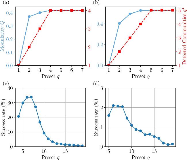
Figure 2. Robustness and search cost of extra community states. (a), (b) The maximum modularity Q (blue, left axis) and the effective number of non-empty communities q* (red, right axis) found by FEM as qset increases. (c), (d) The success rate of FEM replicas finding the exact ground state over 10 000 tests for different qset values. (a), (c) Zachary’s Karate Club and (b), (d) the Dolphins social network. |
2.2. Free energy formulation via variational inference
To effectively navigate the rugged energy landscape defined by the Potts energy in equation (2 ), we employ the FEM framework [17]. FEM approximates the intractable Boltzmann distribution PB(σ, β) ∝ e−βE(σ) using a tractable mean-field variational distribution PMF(σ). Consistent with the mean-field approximation, we assume the spins are statistically independent, leading to the factorized form ${P}_{\,\rm{MF}\,}({\boldsymbol{\sigma }})={\prod }_{i=1}^{N}{p}_{i,{\sigma }_{i}}$, where ${p}_{i,{\sigma }_{i}}$ is the probability that node i is in community σi.
The optimization is theoretically grounded in minimizing the reverse Kullback–Leibler (KL) divergence, DKL(PMF∣∣PB). As derived in the FEM framework, minimizing this divergence is equivalent to minimizing the variational free energy:
$\begin{eqnarray}{{ \mathcal F }}_{\rm{MF}\,}={U}_{\rm{MF}}-\frac{1}{\beta }{S}_{\,\rm{MF}},\end{eqnarray}$
where ${S}_{\,\rm{MF}\,}=-{\sum }_{i,{\sigma }_{i}}{p}_{i,{\sigma }_{i}}\mathrm{ln}{p}_{i,{\sigma }_{i}}$ is the Shannon entropy given mean-field solution.The crucial component is the internal energy $U({\boldsymbol{P}})={\langle E({\boldsymbol{\sigma }})\rangle }_{{P}_{\,\rm{MF}\,}}$. Substituting the modularity energy function E(σ) = −∑i,j Bij δ(σi, σj) into the expectation of the mean-field solution requires careful handling of diagonal terms For different nodes i ≠ j, the expectation is $\langle \delta ({\sigma }_{i},{\sigma }_{j})\rangle ={\sum }_{\sigma =1}^{q}{p}_{i,\sigma }{p}_{j,\sigma }$. However, for self-interactions i = j, $\delta ({\sigma }_{i},{\sigma }_{i})={\sum }_{\sigma =1}^{q}{p}_{i,\sigma }\equiv 1$ regardless of the configuration. Thus, the expected energy is: A for details of the derivation.
$\begin{eqnarray}U({\boldsymbol{P}})=-\displaystyle \sum _{i\ne j}{B}_{ij}\displaystyle \sum _{\sigma =1}^{q}{p}_{i,\sigma }{p}_{j,\sigma }-\displaystyle \sum _{i=1}^{N}{B}_{ii}.\end{eqnarray}$
The second term represents the constant self-energy contribution and does not affect the optimization landscape. The variational structure depends exclusively on the pairwise interactions between distinct nodes. Refer to appendix 2.3. Optimization and complexity
The minimization of the free energy is performed with respect to the mean-field parameters ${\boldsymbol{H}}=\{{h}_{i,{\sigma }_{i}}\}$, which determine the probabilities with a softmax function ${p}_{i,{\sigma }_{i}}=\exp ({h}_{i,{\sigma }_{i}})/{\sum }_{\sigma =1}^{q}\exp ({h}_{i,\sigma })$. The gradient of the free energy with respect to the probabilities, ${{\rm{\nabla }}}_{{\boldsymbol{P}}}{ \mathcal F }$, drives the optimization.
Differentiating the correct internal energy form in equation (4 ) with respect to ${p}_{i{\sigma }_{i}}$, we note that the summation runs only over j ≠ i. Since Bij = Bji, we obtain: A .
$\begin{eqnarray}\frac{\partial U}{\partial {p}_{i{\sigma }_{i}}}=-2\displaystyle \sum _{j\ne i}{B}_{ij}{p}_{j{\sigma }_{i}}.\end{eqnarray}$
Combining this with the entropy derivative, the total explicit gradient is: $\begin{eqnarray}\frac{\partial { \mathcal F }}{\partial {p}_{i{\sigma }_{i}}}=-2\displaystyle \sum _{j\ne i}{B}_{ij}{p}_{j{\sigma }_{i}}+\frac{1}{\beta }(\mathrm{ln}{p}_{i{\sigma }_{i}}+1).\end{eqnarray}$
Critically, the summation in the gradient excludes the self-loop term ${B}_{ii}{p}_{i{\sigma }_{i}}$, which would erroneously appear if one blindly applied the derivative to a full quadratic form P ⊤ B P. The relation between $\frac{\partial { \mathcal F }}{\partial {h}_{i{\sigma }_{i}}}$ and $\frac{\partial { \mathcal F }}{\partial {p}_{i{\sigma }_{i}}}$ has been derived in [17], and is displayed in appendix We integrate these explicit gradients into a gradient-based optimizer (e.g. Adam [21] and SGD [22]) to iteratively update the fields H, following an annealing schedule for β. Regarding the implementation strategy, the original FEM study [17] demonstrated that while automatic differentiation (AD) offers flexibility, it typically requires approximately twice the execution time compared to optimized explicit gradients due to computational graph overhead. We also validate this conclusion on the community detection task (detailed in appendix B ). Consequently, to prioritize computational efficiency for large-scale networks, we strictly employ the explicit sparse gradient formulation described above in our main algorithm.
2.4. Algorithm summary
The FEM-based community detection procedure is outlined in Algorithm 1 . A key feature of our implementation is the use of Nrep parallel replicas, initialized with random fluctuations to explore distinct regions of the energy landscape simultaneously. The algorithm proceeds through an inverse-proportional annealing schedule [17], updating the fields through Nstep steps using a linear cooling in terms of temperature. In the inverse-proportional scheduling, the temperature after nstep steps is T(nstep) = 1/β(nstep) = nstep δT + 1/βmin, where δT = (1/βmin − 1/βmax)/(Nstep − 1) is step size, βmin and βmax are the start and end points of reverse temperature β respectively.
To achieve state-of-the-art performance, we do not rely on default hyperparameters. Instead, we perform a systematic tuning of the optimization parameters, including the learning rate η and optimizer-specific coefficients (e.g. β1, β2 for Adam, or momentum factors for SGD). We observe that different networks require distinct parameter sets to balance convergence speed and solution quality. For instance, larger or denser networks may benefit from more conservative learning rates to prevent oscillation, while the annealing steps Nstep is adjusted to ensure sufficient exploration time before the system undergoes the phase transition from the disordered state to the structured community definition.
Upon convergence, the final partition is selected by evaluating the modularity Q for each replica and choosing the configuration corresponding to the maximum Q.
FEM for Community Detection with Replicas
| Require: Adjacency A, Community numbers qset, Replicas Nrep, field factor h. |
| Require: Annealing: βmin, βmax, Nstep. |
| Require: Optimizer: Type (e.g., Adam, RMSprop, SGD), Learning rate η, Parameters Θ. |
| Ensure: Best community assignment σ *. |
| 1: Precompute: Degrees k, total edges m, inverse annealing step size δT. |
| 2: Initialize: Batch fields ${\boldsymbol{H}}\sim { \mathcal N }(0,{h}^{2})$ of shape (Nrep, N, qset). |
| 3: β ← βmin |
| 4: for step =1 to Nstep do |
| 5: ${p}_{i{\sigma }_{i}}^{(r)}\leftarrow \,\rm{softmax}\,({h}_{i{\sigma }_{i}}^{(r)})$ |
| 6: Compute sparse gradients ${{\rm{\nabla }}}_{{\boldsymbol{H}}}{ \mathcal F }$. |
| 7: Update H using selected optimizer with η, Θ. |
| 8: β ← 1/(1/β − δT) |
| 9: end for |
| 10: Decode: ${\sigma }_{i}^{(r)}\leftarrow \arg \mathop{\max }\limits_{{\sigma }_{i}}{p}_{i,{\sigma }_{i}}^{(r)}$. |
| 11: Select: ${r}^{* }\leftarrow \arg \mathop{\max }\limits_{r}Q({{\boldsymbol{\sigma }}}^{(r)})$. |
| 12: return ${{\boldsymbol{\sigma }}}^{({r}^{* })}$. |
3. Results
To rigorously evaluate the performance of FEM in maximizing modularity, we conducted a comparative analysis against a diverse set of state-of-the-art algorithms. These include widely adopted agglomerative heuristics such as Louvain [9], and Leiden [10]; the combinatorial optimization algorithm Combo [23]; physics-inspired methods including BP [14] and the Rb-pots spin glass solver [13] with same CD-Potts transformation; and the exact integer-programming solver Bayan [7].
All experiments were performed on unweighted and undirected networks. For the exact solver Bayan, which serves as a ground-truth baseline for tractable instances, we imposed a convergence threshold of 10−3 and a computational time limit of 48 h; instances exceeding this duration were marked as intractable. For FEM, the hyperparameters—specifically the annealing schedule (${\beta }_{\min },{\beta }_{\max }$) and the number of parallel replicas (Nrep)—were selected to balance exploration depth with computational cost. Detailed parameter configurations for each dataset are provided in appendix D .
The evaluation is structured to probe the physical limits of the solver: We first examine the method’s robustness to model selection, then analyze in synthetic landscapes (SBM, LFR, ABCD), and finally demonstrate optimization performance on complex real-world networks.
3.1. Robustness to model selection and complexity trade-offs
A key difference between FEM and standard heuristic methods (like Louvain and Leiden) lies in the solution space. While heuristics find the number of communities automatically [24], FEM needs a set maximum number of states, which we denote as qset. This naturally raises a critical requirement, while FEM with an insufficient qset cannot find the true optimal, FEM requires a qset larger than the community number of true optima q*. And the performance of FEM with redundant qset is also important.
We evaluate FEM on two canonical benchmarks: Zachary’s Karate Club and the Dolphins social network. We set the input qset from 1 up to qset = 20, which is significantly larger than the actual community count. As illustrated in figures 2(a) and (b), FEM exhibits a ‘vacuum alignment’ effect common in statistical physics. When qset exceeds the intrinsic number of modules q*, the replicas of FEM naturally find the true optima in the redundant solution space where the extra spin states have zero probability. Consequently, the algorithm converges to the optimal effective number of communities (q* = 4 for Karate, q* = 5 for Dolphins). This confirms that FEM effectively filters out redundant dimensions and does not require precise prior knowledge of q*.
To quantify this, we analyzed the probability of FEM replicas finding the optimal partition on both networks for different values of qset. As shown in figures 2(c) and (d), the success rate first increases with qset and then declines. This indicates a trade-off that while a excessively large state space exponentially expands the search volume and hinders convergence to the exact vacuum-aligned ground state, a moderately redundant qset actually smooths the energy landscape. These extra states act as escape routes to help FEM replica avoid local minima. Thus, a slightly over-parameterized qset effectively optimizes the balance between landscape traversability and state-space complexity.
However, this robustness imposes a thermodynamic cost governed by the expansion of the configuration space. The size of the solution space scales with the system size N as ${({q}_{\,\rm{set}\,})}^{N}$. While the true optimal partition remains stable, the search complexity required to locate it increases with qset.
3.2. Application on synthetic benchmarks
To evaluate the optimization power of FEM under varying degrees of landscape ruggedness, we test it on three synthetic benchmarks: the SBM, the LFR model, and the ABCD. While theoretical studies indicate the existence of detectability phase transitions in these models, our focus here is on the comparative performance trend as the community structure becomes progressively obscured by noise.
3.2.1. Performance on the stochastic block model
We first employ the SBM [18], a canonical generative model known for exhibiting a sharp detectability phase transition. In this model, the difficulty of the community detection task is tightly controlled by the intra-community edge probability (Pin) and the inter-community edge probability (Pout). We define the noise parameter as the ratio ε = Pout/Pin. As ε increases toward 1, the network undergoes a phase transition from an ‘easy’ phase, where the planted community structure is distinct and the energy landscape is smooth, to a ‘hard’ or glassy phase near the theoretical detectability limit, where the true structure is heavily obscured by topological noise. The primary purpose of our SBM experiments is to systematically test FEM’s optimization performance across these varying levels of difficulty.
Using the 300-node networks (q = 3), we analyze the stability of the obtained partitions as ε for different baseline values of Pin. In the low-noise regime (ε ≤ 0.4), the modularity landscape is relatively smooth. Consequently, both FEM and standard heuristic algorithms (such as Louvain and Leiden) reliably identify the optimal partition. However, as the noise increases (ε ≥ 0.6), the optimization problem becomes significantly harder. The energy landscape grows rough, populated with numerous suboptimal local minima. For example, in sparse networks (Pin = 0.1) at ε = 0.6, standard heuristics like Louvain become trapped in shallow minima (QLouvain ≈ 0.187). In contrast, FEM effectively utilizes its replica-based thermal fluctuations to escape these traps, consistently locating a deeper ground state (QFEM ≈0.206). This performance gap widens as the system approaches the highly noisy limit (ε = 0.8), highlighting FEM’s ability to navigate complex spaces where greedy agglomeration methods fail.
To further illustrate the relationship between optimization difficulty and theoretical network limits, we map our experimental results onto the ε–Pin phase diagram (figure 3). The solid curve represents the theoretical detectability threshold, which separates the detectable ordered phase from the noisy regime. We mark the points of experiments by whether FEM uniquely achieves the highest modularity for each experimental instance.
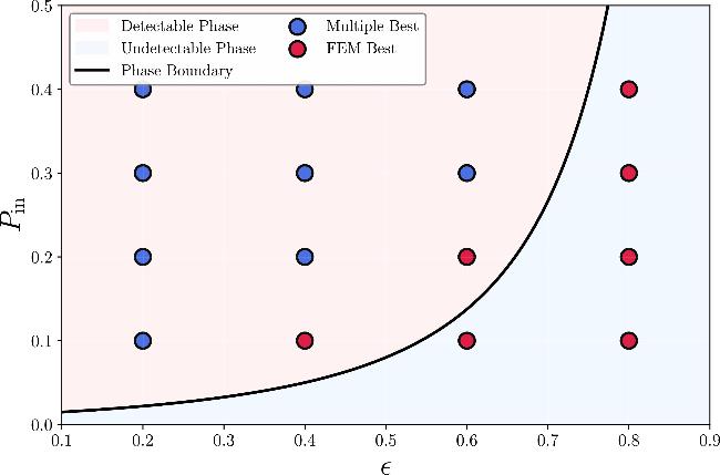
Figure 3. Optimization performance across the SBM phase diagram. The theoretical detectability threshold (solid line) divides the parameter space into detectable and undetectable phases. The scatter points represent experimental instances, categorized by whether FEM uniquely achieves the highest modularity (e.g. red markers) or whether other heuristic methods also find the optimal solution (e.g. blue markers). The distribution demonstrates that as the system approaches the rough energy landscape near the theoretical phase boundary, standard algorithms fail, allowing FEM to demonstrate a distinct optimization advantage. |
As depicted in the figure, in the region far above the transition curve (the easy phase), the energy landscape is smooth enough that multiple algorithms successfully find the ground state. However, as the network parameters approach the theoretical boundary, the optimization landscape becomes highly frustrated. In this rugged regime, standard heuristics become trapped in local minima, and FEM frequently emerges as the uniquely optimal solver. This trend is highly consistent with statistical physics theory: while the region where FEM shows a unique advantage does not perfectly overlap with the exact phase transition line, its superiority is clearly activated by the onset of the glassy landscape near the detectability limit.
Furthermore, SBM experiments reveal a critical limitation of exact optimization methods. As the network connections become more complex, the computational time required by the Bayan solver increases exponentially. In table 1, the instances marked with ‘–’, Bayan failed to process a single network within a 48 h window, whereas FEM and the heuristic algorithms completed the task in less than one second. This stark contrast highlights the severe computational cost of using exact solvers on complex networks. Therefore, for the subsequent experiments, we set a strict 2 h time limit for the Bayan algorithm.
Table 1. The optimal partition of SBM networks obtained by FEM and other algorithms. For each algorithm, the first value corresponds to the maximum modularity Q obtained across multiple runs, and the second value indicates the associated number of communities q, where the optimal result in each network with maximum modularity is highlighted in bold. |
| ε | Pin | Louvain | Combo | Leiden | BP | Rb-pots | FEM | Bayan | Planted |
|---|---|---|---|---|---|---|---|---|---|
| 0.2 | 0.1 | 0.36784, 3 | 0.36784, 3 | 0.36784, 3 | 0.36776, 3 | 0.36784, 3 | 0.36784, 3 | 0.36784, 3 | 0.36721 |
| 0.2 | 0.2 | 0.37920, 3 | 0.37920, 3 | 0.37920, 3 | 0.37920, 3 | 0.37920, 3 | 0.37920, 3 | 0.37920, 3 | 0.37920 |
| 0.2 | 0.3 | 0.37487, 3 | 0.37487, 3 | 0.37487, 3 | 0.37487, 3 | 0.37487, 3 | 0.37487, 3 | 0.37487, 3 | 0.37487 |
| 0.2 | 0.4 | 0.37184, 3 | 0.37184, 3 | 0.37184, 3 | 0.37184, 3 | 0.37184, 3 | 0.37184, 3 | 0.37184, 3 | 0.37184 |
| 0.4 | 0.1 | 0.22665, 8 | 0.23979, 5 | 0.23256, 7 | 0.21375, 3 | 0.22910, 8 | 0.24162, 6 | 0.23607, 5 | 0.21087 |
| 0.4 | 0.2 | 0.21641, 3 | 0.21641, 3 | 0.21641, 3 | 0.21641, 3 | 0.21641, 3 | 0.21641, 3 | 0.21641, 3 | 0.21527 |
| 0.4 | 0.3 | 0.21871, 3 | 0.21871, 3 | 0.21871, 3 | 0.21871, 3 | 0.21871, 3 | 0.21871, 3 | 0.21871, 3 | 0.21871 |
| 0.4 | 0.4 | 0.21960, 3 | 0.21960, 3 | 0.21960, 3 | 0.21960, 3 | 0.21960, 3 | 0.21960, 3 | 0.21960, 3 | 0.21937 |
| 0.6 | 0.1 | 0.18726, 8 | 0.20385, 5 | 0.19404, 7 | −0.01832, 8 | 0.19396, 8 | 0.20566, 6 | 0.19745, 5 | 0.11364 |
| 0.6 | 0.2 | 0.13007, 7 | 0.14061, 4 | 0.13385, 5 | 0.00084, 8 | 0.13329, 6 | 0.14082, 5 | 0.13709, 4 | 0.12151 |
| 0.6 | 0.3 | 0.12077, 4 | 0.12111, 3 | 0.12111, 3 | −0.00610, 4 | 0.12111, 3 | 0.12111, 3 | 0.12098,3 | 0.11654 |
| 0.6 | 0.4 | 0.11876, 3 | 0.11876, 3 | 0.11876, 3 | 0.11848, 3 | 0.11876, 3 | 0.11876, 3 | — | 0.11779 |
| 0.8 | 0.1 | 0.16945, 7 | 0.18132, 5 | 0.17493, 7 | 0.00218, 8 | 0.17378, 7 | 0.18418, 6 | 0.18041, 5 | 0.04111 |
| 0.8 | 0.2 | 0.11184, 7 | 0.11896, 5 | 0.11530, 6 | −0.01158, 6 | 0.11400, 7 | 0.12093, 5 | 0.11660, 4 | 0.05315 |
| 0.8 | 0.3 | 0.08677, 6 | 0.09001, 4 | 0.08545, 5 | −0.00075, 3 | 0.08651, 6 | 0.09105, 4 | 0.08773, 3 | 0.04771 |
| 0.8 | 0.4 | 0.06946, 6 | 0.07214, 4 | 0.07008, 5 | 0.00000, 1 | 0.06915, 6 | 0.07383, 5 | — | 0.04948 |
3.2.2. Robustness on heterogeneous topologies
While the SBM provides a clean theoretical baseline, real-world networks have heavy-tailed degree distributions that introduce significant structural heterogeneity. This irregularity can distort the energy landscape, creating traps for optimization algorithms that rely on local edge density. To validate FEM under realistic conditions, we evaluate it on the LFR [19] (N = 1000) and the ABCD [20] (N = 600) benchmarks. Both models generate networks with power-law distributions for node degrees and community sizes. The structural difficulty is controlled by a noise parameter: the mixing parameter μ for LFR and ABCD.
We generate LFR benchmarks with N = 1000 nodes, average degree ⟨k⟩ = 15, and power-law distributions for both degree (τ1 = 3) and community size (τ2 = 2). And the ABCD benchmarks have N = 600 nodes with power-law distributions for both degree (τ1 = 3) and community size (τ2 = 2). Minimum degree dmin = 10 and maximum degree dmax = 40. We incrementally increased the noise parameters from 0.4 to 0.8. As illustrated in figure 4, the optimization trend mirrors that of the SBM. When the communities are well-defined (e.g. μ ≤ 0.5), the performance of all algorithms is similar. However, as the noise parameters increase beyond 0.6, the internal links become sparse, and the structural heterogeneity begins to severely distort the local energy gradients. In this noisy regime, the obtained modularity of greedy heuristics drops quickly, as they struggle to differentiate structural hubs from true community cores. Conversely, FEM’s global optimization strategy and annealing schedule allow it to maintain a significantly higher accuracy. By effectively filtering out the noise caused by degree heterogeneity, FEM demonstrates strong robustness and superiority in the rugged landscapes typical of complex networks.
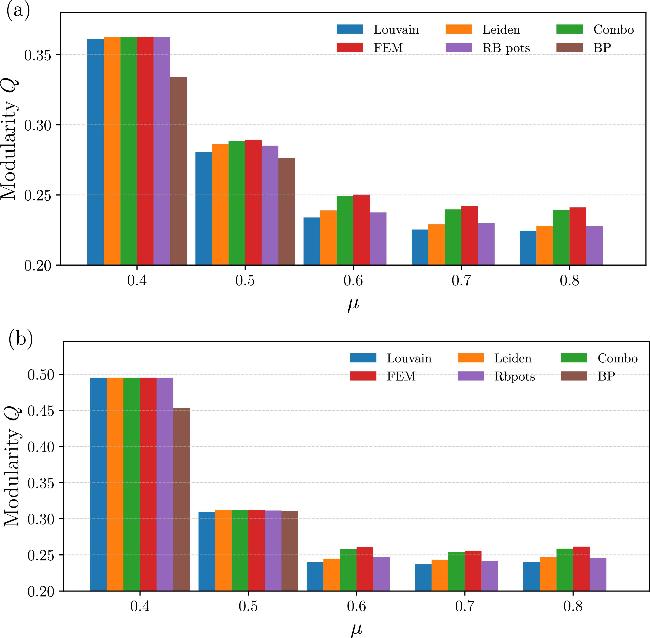
Figure 4. Performance on heterogeneous synthetic benchmarks. (a) Results on the LFR benchmark networks with N = 1000 nodes as a function of the mixing parameter μ. (b) Results on the ABCD benchmark networks with N = 600 nodes across varying mixing parameter μ. In both benchmarks, all algorithms perform similarly in the low-noise regime (μ ≤ 0.5). However, as the noise parameter increases (μ ≥ 0.6), the accuracy of standard heuristic methods drops sharply, whereas FEM maintains a significantly higher performance. |
3.3. Application to real-world networks
Having established the robustness of FEM on synthetic energy landscapes, we now evaluate its performance on a diverse collection of empirical networks. For this analysis, we selected widely studied real-world datasets from the publicly accessible Netzschleuder repository [25].
As summarized in table 2, we compare the maximum modularity obtained by FEM against other solvers. The empirical results indicate that no single algorithm consistently guarantees the global optimum across all network topologies. However, FEM demonstrates the highest success rate in identifying the partitions with the maximum known modularity.
Table 2. Results over the classic network examples. n denotes the number of nodes and m the number of edges. For each algorithm, the first value represents the maximum modularity Q obtained across multiple runs, and the second value is the corresponding number of communities q. For each network, the best result is highlighted in bold. |
| Network | n | m | Louvain | Combo | Leiden | BP | Rb_pots | FEM | Bayan |
|---|---|---|---|---|---|---|---|---|---|
| karate | 34 | 78 | 0.41979, 4 | 0.41979, 4 | 0.41979, 4 | 0.37147, 2 | 0.41979, 4 | 0.41979, 4 | 0.41979, 4 |
| plant_pol | 39 | 42 | 0.56689, 6 | 0.56689, 6 | 0.56689, 6 | -0.15420, 8 | 0.56689, 6 | 0.56689, 6 | 0.56689, 6 |
| sp_kenyan | 47 | 506 | 0.24714, 3 | 0.24714, 3 | 0.24714, 3 | 0.22925, 2 | 0.24714, 3 | 0.24714, 3 | 0.24656, 3 |
| dolphins | 62 | 159 | 0.52852, 5 | 0.52852, 5 | 0.52852, 5 | 0.39538, 2 | 0.52852, 5 | 0.52852, 5 | 0.52852, 5 |
| terrorists_911 | 62 | 152 | 0.53400, 6 | 0.53610, 6 | 0.53610, 6 | 0.50136, 3 | 0.53610, 6 | 0.53610, 6 | 0.53610, 6 |
| law_firm | 71 | 1008 | 0.22537, 3 | 0.22537, 3 | 0.22537, 3 | 0.22537, 3 | 0.22537, 3 | 0.22537, 3 | 0.22537, 3 |
| polbooks | 105 | 441 | 0.52724, 5 | 0.52724, 5 | 0.52724, 5 | 0.52078, 3 | 0.52724, 5 | 0.52724, 5 | 0.52724, 5 |
| football | 115 | 613 | 0.60457, 10 | 0.60457, 10 | 0.60457, 10 | 0.57353, 6 | 0.60457, 10 | 0.60457, 10 | 0.60457, 10 |
| dom | 151 | 1882 | 0.44255, 3 | 0.44255, 3 | 0.44255, 3 | 0.43836, 3 | 0.44255, 3 | 0.44255, 3 | 0.44255, 3 |
| email_company | 167 | 3251 | 0.14030, 4 | 0.14030, 4 | 0.14030, 4 | 0.05932, 5 | 0.14030, 4 | 0.14030, 4 | 0.13396, 4 |
| jazz | 198 | 2742 | 0.44514, 4 | 0.44447, 3 | 0.44514, 4 | 0.44406, 3 | 0.44514, 4 | 0.44514, 4 | 0.44447, 3 |
| contact | 274 | 2124 | 0.13780, 7 | 0.14574, 7 | 0.14366, 7 | −0.13613, 4 | 0.14403, 8 | 0.14574, 7 | 0.14273, 7 |
| celegans | 297 | 2148 | 0.40535, 6 | 0.40624, 4 | 0.40624, 5 | 0.40400, 4 | 0.40627, 5 | 0.40629, 5 | 0.40415, 5 |
| webkb | 434 | 15231 | 0.26591, 4 | 0.26591, 3 | 0.26591, 4 | 0.26325, 3 | 0.26591, 4 | 0.26591, 4 | — |
| dnc | 548 | 10429 | 0.44383, 32 | 0.443866, 16 | 0.443867, 32 | 0.44091, 5 | 0.443867, 32 | 0.443862, 13 | — |
Consistent with our observations on the synthetic benchmarks, the exact integer-programming solver Bayan scales poorly; as the network size and edge density increase, securing a converged solution within a practical timeframe becomes intractable. In contrast, FEM provides a tractable, physics-grounded alternative. By adjusting the thermodynamic hyperparameters—specifically the number of parallel replicas and annealing steps—FEM allows for a flexible balance between computational efficiency and search accuracy.
However, we also observe a specific limitation of the current FEM framework when applied to networks characterized by a massive number of underlying communities. For instance, in the dnc network, where other heuristic methods (e.g. Leiden) identified an optimal partition consisting of 32 communities, FEM failed to reach the absolute maximum modularity, even when initialized with a sufficiently large state space (qset). The physical mapping of community partitions to Potts spin configurations introduces an inherent permutation symmetry. As the intrinsic number of communities q* grows—necessitating a proportionally larger qset—the number of degenerate spin configurations and suboptimal local minima proliferates factorially. Consequently, in networks requiring high-q partitions, the sheer volume of this highly degenerate energy landscape traps the parallel replicas, preventing FEM from effectively breaking symmetry and settling into the true global optimum.
3.4. Computational complexity and scalability
While FEM demonstrates a robust capacity to navigate rugged energy landscapes, evaluating its practical utility requires a careful analysis of its computational complexity relative to established baselines. A comprehensive reporting of execution times across all datasets is provided in appendix D .
When comparing execution times, it is important to contextualize the underlying hardware paradigms: standard agglomerative heuristics (such as Louvain and Leiden) are sequential by nature and are executed on CPUs, whereas FEM leverages GPU acceleration to compute dense matrix multiplications for its mean-field updates. Under our standard hyperparameter configurations—designed to balance exploration depth with efficiency—the computational cost of FEM is highly competitive. Although typically slightly slower than the greedy heuristics, the runtime of FEM remains within the same order of magnitude. For instance, on standard networks (N ∼ 103), both methods generally converge in seconds. This demonstrates that transitioning from a discrete local search to a continuous free-energy optimization does not impose a prohibitive bottleneck for typical applications.
To visually illustrate this trade-off, figure 5 presents the time-quality Pareto front across networks with varying landscape roughness. As shown in the figure, greedy heuristics are exceptionally fast but frequently fall into suboptimal traps in the glassy phase. Exact solvers like Bayan can find the true ground state but scale exponentially, failing on larger or denser instances. FEM occupies a critical middle ground: it consistently recovers high-modularity partitions in structurally noisy regimes, requiring an execution time that is only a constant-factor increase over fast heuristics, while remaining orders of magnitude faster than exact global optimizers.
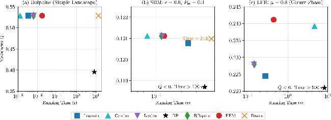


Figure 5. Time-quality pareto front across different energy landscapes. The performance of various algorithms plotted as Modularity Q versus execution time (log scale). (a) On the simple Dolphins network, most algorithms easily find the ground state, illustrating the baseline computational cost. FEM operates in the intermediate time regime between fast heuristics and the exponentially slow exact solver (Bayan). (b) In the intermediate glassy regime of the SBM (ε = 0.6, Pin = 0.3), greedy heuristics are trapped in local optima, while FEM efficiently navigates the landscape to find the deepest ground state faster than the exact solver. (c) In the highly heterogeneous and noisy LFR network (μ = 0.8), the structural noise completely obscures the global optimum from agglomerative methods. FEM remains the only solver capable of recovering the high-modularity partition, requiring only a modest, constant-factor increase in execution time relative to classical heuristics. |
4. Discussion
In this work, we have presented a physics-informed optimization approach for community detection by rigorously mapping the modularity maximization problem to the ground-state search of a Potts spin-glass model. Unlike heuristic methods that treat modularity merely as an arbitrary objective function to be optimized via local moves, our formulation leverages the exact physical equivalence between the modularity matrix and the coupling interactions of a disordered system. A central contribution of this study is the analytical derivation of the explicit gradients for the mean-field variational free energy corresponding to this specific energy. This theoretical step enables the application of the FEM framework, transforming the discrete combinatorial problem into a continuous, differentiable optimization task. By driving the system with these physically grounded gradients, our method effectively navigates the rugged energy landscapes characteristic of complex networks. The experimental results confirm that this approach successfully identifies high-quality partitions, particularly in ‘glassy’ regimes where the community structure is obscured by noise or heterogeneity, offering a rigorous alternative to standard agglomerative heuristics.
The superiority of FEM in the high-noise regime of the SBM and LFR benchmarks highlights the fundamental advantage of statistical physics approaches over greedy agglomeration. In the ‘easy’ phase, where the community structure is unambiguous, the energy landscape is relatively smooth, allowing local heuristics like Louvain and Leiden to converge rapidly to the global optimum. However, as the mixing parameter increases, the landscape undergoes a phase transition, becoming fractured with numerous metastable states (local optima) separated by high energy barriers. Greedy algorithms, lacking a mechanism to accept transient energy increases, typically freeze into these suboptimal configurations. In contrast, FEM employs a deterministic annealing schedule combined with parallel replica evolution. This thermal exploration allows the system to traverse potential barriers and avoid premature trapping in shallow minima, thereby accessing deeper ground states that correspond to partitions with higher modularity.
A practical advantage of our formulation is its inherent robustness to model selection, specifically regarding the number of communities qset given to FEM. Standard spectral or inference-based methods often require precise estimation of q* to avoid under- or over-fitting. Our experiments demonstrate that FEM exhibits a ‘vacuum alignment’ property: when initialized with a surplus of spin states (qset > q*), the variational optimization naturally suppresses the occupancy probability of redundant states to zero. However, it is crucial to note that this vacuum alignment is not strictly deterministic within a single trajectory but rather emerges probabilistically across parallel replicas. An excessively redundant spin space exponentially expands the configuration volume, which, as shown in our experiments, decreases the probability that a given replica spontaneously converges to the correct vacuum-aligned ground state. Consequently, extreme over-parameterization incurs a higher computational cost, requiring more replicas to adequately sample the expanded landscape. This suggests that while FEM is robust, operating with a suitably low qset is practically advantageous, making the development of adaptive qset-selection schemes—akin to traditional agglomerative algorithms—a promising direction. Interestingly, our results also reveal a nuanced dynamic: a moderately relaxed state space (a slightly redundant qset) can sometimes increase the probability of locating the true optimum. We hypothesize that these extra dimensions may act as ‘escape routes’ that effectively reduce the ruggedness of the local energy landscape. A systematic theoretical exploration of this dimensional smoothing effect is left for future work.
While FEM consistently outperforms state-of-the-art heuristics across the majority of benchmark networks, it is essential to recognize its fundamental limitations, particularly concerning networks with a large intrinsic number of communities (q*). As observed in our empirical evaluations, when the optimal partition requires a high q*, the necessary expansion of the spin state space qset induces a combinatorial explosion of degenerate local minima. This extreme degeneracy severely hinders the replicas from navigating to the exact global ground state. Due to the stochastic nature of the variational optimization and the extreme roughness of the modularity landscape, escaping these massive degenerate traps relies heavily on the allocated computational budget. Significantly relaxing resource constraints, such as increasing the number of replicas and annealing steps by an order of magnitude, may uncover partitions with marginally higher modularity. However, accessing these deeper ground states requires a disproportionate increase in execution time. This observation suggests a critical avenue for future research: breaking the permutation symmetry or improving the search efficiency of the FEM framework to navigate highly degenerate energy landscapes more effectively, thereby reducing the reliance on brute-force computational scaling.
Looking forward, the differentiable nature of the FEM framework opens several avenues for methodological extension. While this study focused on the standard modularity function for undirected, unweighted graphs, the gradient-based formulation can be readily adapted to more complex energy functions, including those for directed networks, overlapping communities, or multi-resolution quality functions. Furthermore, since the core computational bottleneck involves dense matrix-vector multiplications for the mean-field updates, the algorithm is well-suited for massive parallelization on modern hardware accelerators such as GPUs and TPUs. Future work will explore integrating FEM with graph neural networks to learn effective initialization strategies, potentially bridging the gap between combinatorial optimization and representation learning.
Appendix A. Derivation of the mean-field internal energy and field gradient
The mean-field internal energy for modularity UMF =−2 m∑ σ PMF( σ)Q( σ) can be simplified by expanding the mean field solution:
$\begin{eqnarray}\begin{array}{rcl}U({\boldsymbol{P}}) & = & -2m\displaystyle \sum _{{\boldsymbol{\sigma }}}\frac{1}{2m}\displaystyle \sum _{i,j}{B}_{ij}\delta ({\sigma }_{i},{\sigma }_{j})\displaystyle \prod _{k}{p}_{k,{\sigma }_{k}}\\ & = & -\displaystyle \sum _{i\ne j}\displaystyle \sum _{\sigma =1}^{q}{B}_{ij}{p}_{i,\sigma }{p}_{j,\sigma }-\displaystyle \sum _{i}\displaystyle \sum _{\sigma =1}^{q}{B}_{ii}{p}_{i,\sigma }\\ & = & -\displaystyle \sum _{i\ne j}\displaystyle \sum _{\sigma =1}^{q}{B}_{ij}{p}_{i,\sigma }{p}_{j,\sigma }-\displaystyle \sum _{i}{B}_{ii}.\end{array}\end{eqnarray}$
Following the function in the supplementary of [17], the derivative of free energy is A1 ), we have: A2 ), we can obtain the explicit gradient $\frac{\partial {F}_{\,\rm{MF}\,}}{\partial {h}_{i,{\sigma }_{i}}}$ to update H.
$\begin{eqnarray}\frac{\partial {F}_{\,\rm{MF}\,}}{\partial {h}_{i,{\sigma }_{i}}}=\left[{\hat{g}}_{i,{\sigma }_{i}}^{\,p}-\displaystyle \sum _{{\sigma }_{i}^{{\prime} }=1}^{q}{p}_{i,{\sigma }_{i}^{{\prime} }}{\hat{g}}_{i,{\sigma }_{i}^{{\prime} }}^{\,p}\right]{p}_{i,{\sigma }_{i}},\end{eqnarray}$
in which ${\hat{g}}_{i,{\sigma }_{i}}^{\,p}=\frac{\partial {F}_{\rm{MF}\,}}{\partial {p}_{i,{\sigma }_{i}}}=\frac{\partial {U}_{\rm{MF}}}{\partial {p}_{i,{\sigma }_{i}}}-\frac{1}{\beta }\frac{\partial {S}_{\,\rm{MF}}}{\partial {p}_{i,{\sigma }_{i}}}$ is the gradient to each mean-field probabilities. The second term of $\frac{\partial {S}_{\,\rm{MF}\,}}{\partial {p}_{i,{\sigma }_{i}}}\,=-\mathrm{ln}{p}_{i,{\sigma }_{i}}-1$ has been derived in [17]. Thus we only need gradient $\frac{\partial {U}_{\,\rm{MF}\,}}{\partial {p}_{i,{\sigma }_{i}}}$. By equation ( $\begin{eqnarray}\frac{\partial {U}_{\,\rm{MF}\,}}{\partial {p}_{i,{\sigma }_{i}}}=-2\displaystyle \sum _{j\ne i}{B}_{ij}{p}_{j,{\sigma }_{i}}.\end{eqnarray}$
Substitute to ${\hat{g}}_{i,{\sigma }_{i}}^{\,p}$ and then equation (Appendix B. Explicit gradient and automatic differentiation
As discussed in the main text, the FEM framework can be implemented using either AD or by analytically deriving the explicit gradients of the variational free energy. While AD offers significant flexibility for rapid prototyping with arbitrary network energy functions, it introduces substantial computational overhead due to the dynamic construction and evaluation of computational graphs during backpropagation. The original FEM study [17] empirically noted that AD typically requires approximately twice the execution time compared to an optimized explicit gradient implementation.
To validate this observation within the specific context of community detection, we compared the runtime of both approaches using the exact hyperparameter configurations that yielded the optimal results presented in section 3 . Table 3 illustrates this runtime comparison across both the SBM networks and the diverse suite of empirical real-world networks.
Table 3. Runtime comparison between explicit gradients and Automatic Differentiation (AD). The execution time of FEM using analytically derived explicit sparse gradients versus AD on SBM networks and real-world empirical networks. The evaluation employs the exact optimal hyperparameters utilized for the main results. Across all instances, the AD approach consistently requires approximately twice the computational time of the explicit gradient method, validating the necessity of our analytical derivations to optimize execution speed. |
| Network | Explicit gradient (s) | Automatic differentiation (s) |
|---|---|---|
| karate | 0.014 23 | 0.039 73 |
| dolphins | 0.017 22 | 0.039 97 |
| celegans | 0.077 06 | 0.175 11 |
| SBM_0.6,0.3 | 0.124 52 | 0.184 99 |
| ABCD_0.6 | 0.337 23 | 0.597 19 |
Consistent with the original findings [17], our results demonstrate that relying on AD roughly doubles the computational time across all tested network topologies and sizes. Crucially, because the analytically derived sparse gradients [as formulated in equation (6 )] are mathematically equivalent to those computed via AD, this acceleration comes with absolutely no loss of optimization accuracy or landscape exploration capability. Consequently, the explicit gradient formulation is strictly adopted in our main algorithm to ensure scalability and high-performance execution on large and complex networks.
Appendix C. Hyperparameter setting of FEM
For each dataset, the FEM was run with a specific hyperparameter configuration, including the annealing schedule $({\beta }_{\min },{\beta }_{\max },{N}_{\,\rm{step}\,})$, the number of parallel replicas Nreplica, the field initialization scale h, and the optimizer together with its associated coefficients. The full set of configurations used in the main experiments is summarized in table 4. Rather than relying on a universal default setting, we selected these parameters to balance exploration depth, optimization stability, and computational efficiency across networks with different sizes, densities, and landscape roughness. In all FEM experiments, computations were performed on an NVIDIA A100 GPU, and all variables were represented in 32-bit single-precision floating-point format. This implementation choice provides an effective compromise between numerical stability, memory usage, and execution speed for large-scale variational optimization.
Table 4. Hyperparameter settings for FEM. Nreplica and Nsteps denote the number of replicas and annealing steps, respectively. RC time refers to the replica computation time when running FEM. |
| Network | ${\beta }_{\min }$ | ${\beta }_{\max }$ | Nsteps | Nreplica | h | Optimizer | lr | Weight decay | ε | β1 | β2 | amsgrad | α | Momentum | Centered | RC time (s) |
|---|---|---|---|---|---|---|---|---|---|---|---|---|---|---|---|---|
| SBM_0.2,0.1 | 0.1 | 10 | 20 | 20 | 0.1 | adam | 1 | 0 | 1e-09 | 0.1 | 0.999 | False | — | — | — | 0.03270 |
| SBM_0.2,0.2 | 0.1 | 10 | 10 | 10 | 0.1 | rmsprop | 0.2 | 0 | 1e-08 | — | — | — | 0.98 | 0 | False | 0.04601 |
| SBM_0.2,0.3 | 0.1 | 1 | 10 | 5 | 0.2 | rmsprop | 0.2 | 0 | 1e-08 | — | — | — | 0.9 | 0 | True | 0.06444 |
| SBM_0.2,0.4 | 0.1 | 1 | 10 | 5 | 0.5 | adam | 1 | 0.0001 | 0.0001 | 0.0 | 0.1 | True | — | — | — | 0.08823 |
| SBM_0.4,0.1 | 0.1 | 10 | 500 | 100 | 0.1 | rmsprop | 0.2 | 0.01 | 1e-08 | — | — | — | 0.9 | 0.99 | False | 0.29696 |
| SBM_0.4,0.2 | 0.01 | 10 | 20 | 10 | 0.1 | rmsprop | 0.2 | 0.0001 | 1e-08 | — | — | — | 0.98 | 0.5 | False | 0.06386 |
| SBM_0.4,0.3 | 0.1 | 10 | 10 | 5 | 0.5 | adam | 1 | 0 | 1e-08 | 0.0 | 0.1 | True | — | — | — | 0.08387 |
| SBM_0.4,0.4 | 0.1 | 1 | 10 | 5 | 0.1 | adam | 1 | 0 | 0.0001 | 0.0 | 0.1 | False | — | — | — | 0.10873 |
| SBM_0.6,0.1 | 0.01 | 10 | 500 | 100 | 0.2 | rmsprop | 0.2 | 0.01 | 1e-08 | — | — | — | 0.95 | 0.99 | False | 0.30505 |
| SBM_0.6,0.2 | 0.01 | 10 | 200 | 50 | 0.1 | rmsprop | 0.2 | 0.0001 | 1e-08 | — | — | — | 0.95 | 0.9 | False | 0.17104 |
| SBM_0.6,0.3 | 0.1 | 10 | 50 | 50 | 0.1 | adam | 1 | 0 | 0.0001 | 0.1 | 0.999 | True | — | — | — | 0.12452 |
| SBM_0.6,0.4 | 0.001 | 10 | 50 | 50 | 1 | adam | 0.1 | 0 | 1e-08 | 0.1 | 0.1 | False | — | — | — | 0.15513 |
| SBM_0.8,0.1 | 0.01 | 10 | 500 | 50 | 0.2 | rmsprop | 0.2 | 0.01 | 1e-08 | — | — | — | 0.9 | 0.99 | False | 0.31425 |
| SBM_0.8,0.2 | 0.01 | 10 | 200 | 50 | 0.1 | rmsprop | 0.2 | 0.01 | 1e-08 | — | — | — | 0.9 | 0.99 | False | 0.18774 |
| SBM_0.8,0.3 | 0.1 | 10 | 100 | 50 | 0.2 | rmsprop | 0.2 | 0 | 1e-08 | — | — | — | 0.9 | 0.5 | True | 0.17788 |
| SBM_0.8,0.4 | 0.01 | 10 | 100 | 50 | 0.1 | rmsprop | 0.2 | 0.01 | 1e-08 | — | — | — | 0.9 | 0.99 | False | 0.21845 |
| | ||||||||||||||||
| LFR_0.4 | 0.1 | 1 | 100 | 50 | 0.2 | rmsprop | 0.2 | 0 | 1e-10 | — | — | — | 0.9 | 0.5 | False | 0.19223 |
| LFR_0.5 | 0.01 | 10 | 200 | 100 | 0.1 | rmsprop | 0.5 | 0.01 | 1e-08 | — | — | — | 0.95 | 0.9 | True | 0.46346 |
| LFR_0.6 | 0.01 | 10 | 200 | 100 | 1.0 | rmsprop | 0.5 | 0.01 | 1e-10 | — | — | — | 0.95 | 0.9 | True | 0.46674 |
| LFR_0.7 | 0.1 | 10 | 200 | 100 | 0.5 | rmsprop | 0.5 | 0.01 | 1e-08 | — | — | — | 0.9 | 0.9 | False | 0.44558 |
| LFR_0.8 | 0.1 | 10 | 200 | 200 | 0.5 | rmsprop | 0.2 | 0 | 1e-08 | — | — | — | 0.9 | 0.9 | True | 0.72154 |
| | ||||||||||||||||
| ABCD_0.4 | 0.001 | 1 | 50 | 50 | 0.2 | rmsprop | 0.5 | 0.01 | 1e-08 | — | — | — | 0.9 | 0.0 | False | 0.07452 |
| ABCD_0.5 | 0.001 | 10 | 100 | 100 | 0.5 | rmsprop | 0.5 | 1e-05 | 1e-08 | — | — | — | 0.9 | 0.5 | True | 0.13014 |
| ABCD_0.6 | 0.1 | 10 | 200 | 200 | 0.1 | rmsprop | 0.5 | 0.01 | 1e-08 | — | — | — | 0.9 | 0.9 | False | 0.33723 |
| ABCD_0.7 | 0.1 | 10 | 200 | 200 | 0.5 | rmsprop | 0.5 | 0.01 | 1e-08 | — | — | — | 0.9 | 0.9 | True | 0.34312 |
| ABCD_0.8 | 0.001 | 10 | 500 | 1000 | 1.0 | rmsprop | 0.5 | 0.01 | 1e-08 | — | — | — | 0.9 | 0.9 | True | 3.15937 |
| | ||||||||||||||||
| karate | 0.001 | 1.0 | 20 | 20 | 0.1 | adam | 1.0 | 0.0 | 1e-8 | 0.0 | 0.1 | False | — | — | — | 0.01423 |
| plant_pol | 0.001 | 1.0 | 20 | 20 | 0.1 | adam | 1.0 | 0.0 | 1e-8 | 0.9 | 0.999 | False | — | — | — | 0.01394 |
| sp_kenyan | 0.001 | 1.0 | 10 | 5 | 0.1 | adam | 0.1 | 0.0001 | 1e-9 | 0.9 | 0.98 | True | — | — | — | 0.01303 |
| terrorists_911 | 0.001 | 1.0 | 20 | 50 | 0.1 | adam | 0.1 | 1e-8 | 1e-16 | 0.1 | 0.999 | True | — | — | — | 0.01563 |
| dolphins | 0.001 | 1.0 | 20 | 50 | 0.1 | adam | 1.0 | 1e-8 | 1e-16 | 0.1 | 0.999 | True | — | — | — | 0.01722 |
| law_firm | 0.001 | 10 | 20 | 20 | 0.5 | adam | 0.1 | 0.0001 | 1e-9 | 0.0 | 0.98 | True | — | — | — | 0.02451 |
| polbooks | 0.001 | 1.0 | 20 | 50 | 0.1 | adam | 1.0 | 1e-8 | 1e-9 | 0.0 | 0.9 | True | — | — | — | 0.02027 |
| football | 0.001 | 1.0 | 50 | 50 | 0.5 | adam | 0.1 | 0.0001 | 1e-9 | 0.0 | 0.98 | True | — | — | — | 0.03957 |
| jazz | 0.001 | 1.0 | 50 | 50 | 0.5 | adam | 1.0 | 0.0001 | 1e-9 | 0.0 | 0.98 | True | — | — | — | 0.05984 |
| dom | 0.001 | 1.0 | 20 | 20 | 0.1 | adam | 0.1 | 0.0001 | 1e-9 | 0.0 | 0.98 | True | — | — | — | 0.03463 |
| email_company | 0.001 | 1.0 | 50 | 20 | 0.1 | adam | 1.0 | 0.0 | 1e-4 | 0.0 | 0.5 | False | — | — | — | 0.06314 |
| celegans | 0.1 | 10 | 100 | 50 | 0.1 | rmsprop | 0.1 | 0.0001 | 1e-8 | — | — | — | 0.9 | 0.5 | False | 0.07706 |
| contact | 0.001 | 10 | 500 | 10000 | 0.1 | rmsprop | 0.2 | 0.01 | 1e-8 | — | — | — | 0.98 | 0.99 | False | 4.87430 |
| webkb | 0.001 | 10 | 200 | 200 | 1.0 | adam | 0.1 | 0.0 | 0.0001 | 0.1 | 0.999 | False | — | — | — | 0.33726 |
| dnc | 0.001 | 1.0 | 400 | 400 | 0.5 | adam | 0.01 | 1e-8 | 1e-8 | 0.0 | 0.9 | False | — | — | — | 2.46268 |
Appendix D. Running time comparison
The running times of FEM and the baseline community-detection algorithms on the SBM, LFR, ABCD, and real-world benchmark datasets are reported in table 5. These results should be interpreted together with the different hardware paradigms of the compared methods: heuristic algorithms such as Louvain and Leiden are sequential CPU-based methods, whereas FEM leverages GPU acceleration for the parallel optimization of mean-field variables. The CPU-based experiments were conducted on an Intel® Core TM i5-14400F @ 2.50 GHz. Under the hyperparameter settings listed in tables 4 and 5, FEM typically remains within the same practical time scale as fast heuristic solvers, while consistently achieving higher-quality solutions in rugged or noisy landscapes; at the same time, it is substantially more scalable than the exact solver Bayan, whose running time becomes prohibitive on larger or denser instances. For the heuristic algorithms, the reported timings were collected over 1000 runs, and bold entries indicate cases in which the corresponding method attains the maximum modularity solution.
Table 5. Time comparison of community detection methods on SBM, LFR, ABCD, and real-world datasets. Data of greedy methods is running 1000 times. Bold entries indicate that the method successfully finds the maximum modularity solution. |
| Dataset | Louvain (s) | Combo (s) | Leiden (s) | BP (s) | Rb-pots (s) | FEM (s) | Bayan (s) |
|---|---|---|---|---|---|---|---|
| SBM 0.2,0.1 | 0.05845 | 0.02394 | 0.03496 | 10.36796 | 0.03477 | 0.03270 | 7707.03 |
| SBM 0.2,0.2 | 0.04946 | 0.01425 | 0.03970 | 17.52000 | 0.03953 | 0.04601 | 47575.12 |
| SBM 0.2,0.3 | 0.05313 | 0.01255 | 0.04497 | 29.04861 | 0.04088 | 0.06444 | 33194.58 |
| SBM 0.2,0.4 | 0.06213 | 0.01347 | 0.05665 | 45.69619 | 0.05588 | 0.08823 | 87614.32 |
| SBM 0.4,0.1 | 0.06441 | 0.14290 | 0.04226 | 61.05834 | 0.04257 | 0.29696 | 4264.82 |
| SBM 0.4,0.2 | 0.10679 | 0.03196 | 0.05825 | 33.04199 | 0.05684 | 0.06386 | 25018.33 |
| SBM 0.4,0.3 | 0.08877 | 0.02136 | 0.06279 | 43.60820 | 0.06229 | 0.08387 | 72418.75 |
| SBM 0.4,0.4 | 0.08928 | 0.02271 | 0.07164 | 69.83765 | 0.07253 | 0.10873 | 133136.02 |
| SBM 0.6,0.1 | 0.07849 | 0.14001 | 0.04934 | 79.66638 | 0.04904 | 0.30505 | 4774.92 |
| SBM 0.6,0.2 | 0.13955 | 0.12424 | 0.07846 | 154.67767 | 0.07744 | 0.17104 | 33072.16 |
| SBM 0.6,0.3 | 0.24032 | 0.07800 | 0.11855 | 119.72449 | 0.11536 | 0.12452 | 89882.57 |
| SBM 0.6,0.4 | 0.20904 | 0.04085 | 0.11444 | 105.38294 | 0.11368 | 0.15513 | — |
| SBM 0.8,0.1 | 0.08977 | 0.12921 | 0.05568 | 92.61624 | 0.05569 | 0.31425 | 6858.19 |
| SBM 0.8,0.2 | 0.15472 | 0.10967 | 0.08672 | 196.45522 | 0.08497 | 0.18774 | 51095.25 |
| SBM 0.8,0.3 | 0.21865 | 0.11378 | 0.11474 | 344.69290 | 0.11235 | 0.17788 | 151295.72 |
| SBM 0.8,0.4 | 0.27872 | 0.10820 | 0.14758 | 523.45163 | 0.14357 | 0.21845 | — |
| | |||||||
| LFR 0.4 | 0.20287 | 3.60421 | 0.11094 | 110.96890 | 0.11169 | 0.19223 | — |
| LFR 0.5 | 0.22764 | 5.22385 | 0.12419 | 240.44396 | 0.12403 | 0.46346 | — |
| LFR 0.6 | 0.26550 | 4.93960 | 0.13844 | 456.16529 | 0.13934 | 0.46674 | — |
| LFR 0.7 | 0.27153 | 4.70492 | 0.13817 | 502.13329 | 0.14117 | 0.44558 | — |
| LFR 0.8 | 0.27264 | 4.64826 | 0.14179 | 502.77521 | 0.14382 | 0.72154 | — |
| | |||||||
| ABCD 0.4 | 0.08159 | 0.13270 | 0.05582 | 45.29087 | 0.05633 | 0.07452 | — |
| ABCD 0.5 | 0.15129 | 0.79663 | 0.08001 | 95.94132 | 0.07926 | 0.13014 | — |
| ABCD 0.6 | 0.14345 | 1.06762 | 0.08101 | 203.25281 | 0.08073 | 0.33723 | — |
| ABCD 0.7 | 0.15377 | 1.02897 | 0.08400 | 205.20803 | 0.08315 | 0.34312 | — |
| ABCD 0.8 | 0.15119 | 1.03868 | 0.08325 | 201.13860 | 0.08182 | 3.15937 | — |
| | |||||||
| karate | 0.00170 | 0.00148 | 0.00400 | 8.53220 | 0.00412 | 0.01423 | 1.45689 |
| plant_pol | 0.00128 | 0.00070 | 0.00350 | 8.42835 | 0.00358 | 0.01394 | 0.86720 |
| sp_kenyan | 0.00426 | 0.00102 | 0.00849 | 11.78332 | 0.00826 | 0.01303 | 29.15627 |
| terrorists_911 | 0.00326 | 0.00175 | 0.00640 | 8.64174 | 0.00587 | 0.01563 | 9.08253 |
| dolphins | 0.00330 | 0.00125 | 0.00634 | 8.22396 | 0.00621 | 0.01722 | 13.31875 |
| law_firm | 0.00850 | 0.00156 | 0.01276 | 19.58261 | 0.01266 | 0.02451 | 183.52224 |
| polbooks | 0.00745 | 0.00625 | 0.01018 | 2.29347 | 0.00980 | 0.02027 | 129.46696 |
| football | 0.00706 | 0.00672 | 0.01036 | 4.10450 | 0.00998 | 0.03957 | 147.92120 |
| jazz | 0.03090 | 0.00891 | 0.02421 | 13.10062 | 0.02463 | 0.05984 | 6701.29833 |
| dom | 0.01895 | 0.00585 | 0.01799 | 8.19518 | 0.01827 | 0.03463 | 701.04215 |
| email_company | 0.04132 | 0.01620 | 0.03208 | 87.34269 | 0.03163 | 0.06314 | 2816.19837 |
| contact | 0.03886 | 0.08597 | 0.02629 | 31.33303 | 0.02647 | 4.87430 | 3368.91957 |
| celegans | 0.04065 | 0.05519 | 0.02800 | 34.32253 | 0.02868 | 0.07706 | 4388.82409 |
| webkb | 0.15897 | 0.05304 | 0.10532 | 173.93826 | 0.10463 | 0.33726 | — |
| dnc | 0.13498 | 1.13962 | 0.08180 | 156.48173 | 0.08201 | 2.46268 | — |