

1. Introduction
2. Previous heuristic algorithms
3. Exact algorithm
3.1. Branch-and-bound framework
3.2. Structural branching strategy: from spins to clusters
| • Scenario 1 (Site Decimation, Sv = −1). The vertex v is removed. This is a strictly local operation, analogous to the standard decimation procedure acting on a single site and its immediate edges. | |
| • Scenario 2 (Cluster Decoupling, Sv = +1). The vertex v is retained. To satisfy the subcritical constraint, v must be confined within a finite cluster ${\mathscr{G}}(v)$ of size $| {\mathscr{G}}(v)| \leqslant C$. This imposes an extended topological constraint: the boundary $\partial {\mathscr{G}}(v)$ must be removed (${{\boldsymbol{S}}}_{u}=-1,\forall u\in \partial {\mathscr{G}}(v)$). |
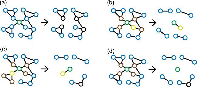
Figure 1. Branching scenarios for network dismantling. The pivot vertex is shown in green; vertices retained together with the pivot as a cluster ${\mathscr{G}}(v)$ are shown in yellow/brown; vertices that must be removed (either the pivot itself or the boundary $\partial {\mathscr{G}}(v)$) are shown in black. The four panels enumerate the branches generated at a single pivot for C = 2. (a) Scenario 1 (Sv = − 1): the pivot is directly removed; recursion then continues on G\{v}. This is a purely local (site-level) move. (b)–(d) Scenario 2 (Sv = + 1): the pivot is retained and must lie inside some connected subgraph ${\mathscr{G}}(v)$ with $| {\mathscr{G}}(v)| \leqslant C$; the entire boundary $\partial {\mathscr{G}}(v)$ is then removed in one mesoscopic step. Panels (b) and (c) show two distinct two-vertex clusters containing the pivot, each producing a different boundary and hence a different child sub-problem; panel (d) shows the degenerate singleton cluster ${\mathscr{G}}(v)=\{v\}$, in which case every immediate neighbour of v must be deleted. Scenarios 1 and 2 together exhaust all configurations of v consistent with the subcritical constraint, guaranteeing completeness of the search tree. |
3.3. Completeness and optimality of the pruning
Branch-and-Bound Dismantling (BD)
| Input: Undirected graph G = (V, E), threshold C, current set Scurr, best solution Smin |
| Output: Updated minimal dismantling set Smin |
| 1: Function BD(G, Scurr) |
| 2: if ∣LCC(G)∣≤C then ⊳Global constraint satisfied |
| 3: if ∣Scurr∣ < ∣Smin∣ then |
| 4: Smin ← Scurr |
| 5: end if |
| 6: return |
| 7: end if |
| 8: Pruning: |
| 9: if ∣Scurr∣≥∣Smin∣ then return |
| 10: end if |
| 11: $v\leftarrow {{\rm{\arg }}\,{\rm{\max }}}_{u\in {\rm{LCC}}(G)}\,{\rm{\deg }}(u)$ ⊳Select pivot vertex |
| 12: Branch 1: Remove v |
| 13: BD(G\{v}, Scurr ∪ {v}) |
| 14: Branch 2: Retain v (Group Isolation) |
| 15: Identify all connected subgraphs $\{{{\mathscr{G}}}_{i}(v)\}$ where $v\in {{\mathscr{G}}}_{i}(v)$ and $| {{\mathscr{G}}}_{i}(v)| \leqslant C$ |
| 16: for each group ${{\mathscr{G}}}_{i}(v)$ do |
| 17: $D\leftarrow \partial {{\mathscr{G}}}_{i}(v)$ ⊳Boundary to remove |
| 18: ${G}^{{\prime} }\leftarrow G\setminus ({{\mathscr{G}}}_{i}(v)\cup D)$ ⊳Remove group and boundary |
| 19: BD(${G}^{{\prime} },{S}_{\,\rm{curr}\,}\cup D$) |
| 20: end for |
| 21: End Function |
3.4. Case study: the 9/11 terrorist network
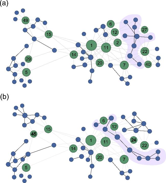
Figure 2. Exact dismantling of the 9/11 terrorist network (C = 9). (a) An initial solution derived from degree-based heuristics (∣S∣ = 15, LCC size = 9). (b) The optimal solution identified by BD (∣S∣ =12). Bold labels indicate key low-degree vertices (e.g., nodes 45 and 24) identified by the exact solver. These vertices serve as critical connectors that are overlooked by heuristics like HD or CI, which produce larger dismantling sets for the same threshold. |
4. Numerical experiments
4.1. Exact results on random graphs
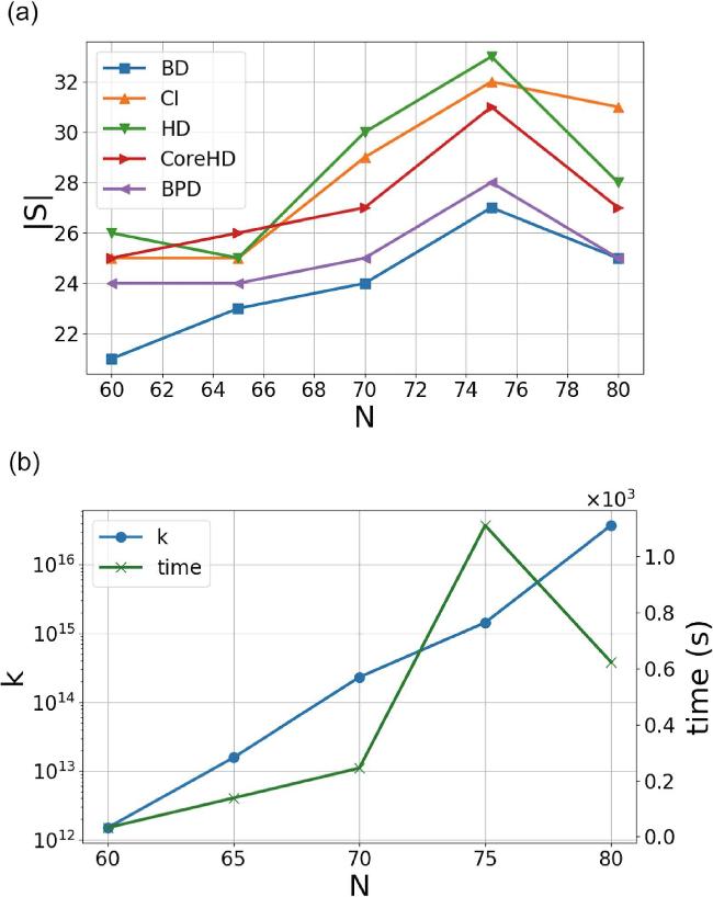
Figure 3. Results on Erdős–Rényi (ER) graphs. Networks were generated with a fixed seed and an average degree ⟨k⟩ = 3.5. (a) Dismantling set size ∣S∣ versus vertex count N. BPD exhibits the best average performance among heuristics. (b) Efficiency of the exact algorithm: k-value (pruning efficiency, blue) and computation time (green) versus N. The slope change in k reflects the transition from C = 3 to C = 4 (maintaining a 5% LCC threshold), illustrating the trade-off between group search complexity and pruning power. |
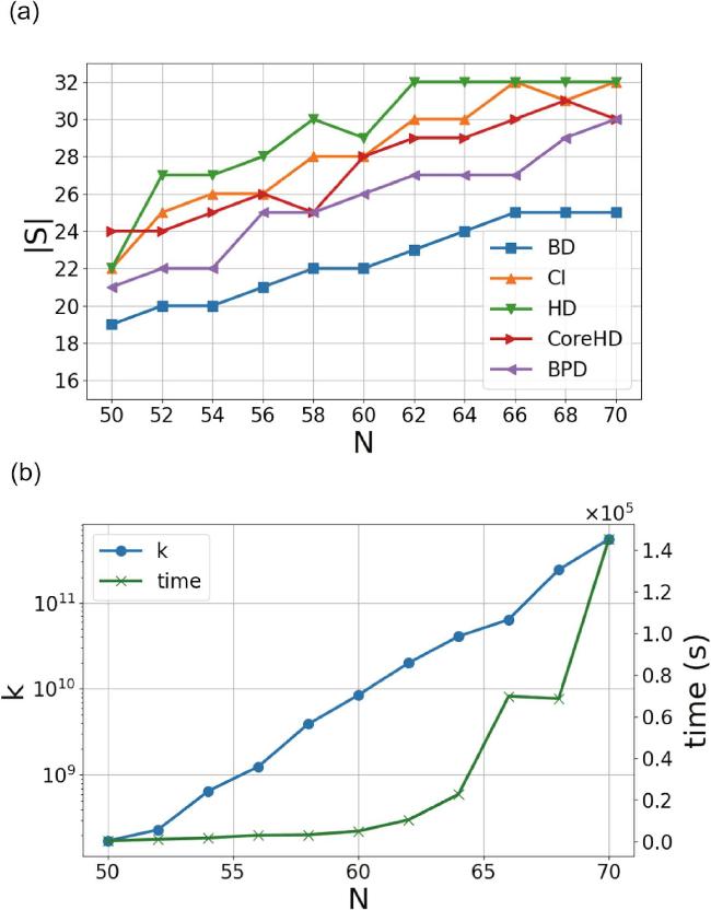


Figure 4. Performance on 4-regular random graphs. (a) Dismantling set size versus vertex count. BPD consistently outperforms other heuristics. (b) Computational metrics for BD: pruning efficiency (k-value) and runtime. The structural homogeneity of regular graphs makes pruning less effective (lower k) compared to ER graphs. |
4.2. Approximation and scalability
Table 1. Performance on 100-vertex Erdős–Rényi graphs (⟨k⟩ = 3.5). BDA denotes our approximate algorithm. Bold values indicate the best found solution. BDA consistently outperforms heuristics while maintaining high computational efficiency. |
| Edges | BDA | CI | HD | CoreHD | BPD |
|---|---|---|---|---|---|
| 162 | 26 | 35 | 35 | 29 | 28 |
| 176 | 29 | 34 | 34 | 33 | 32 |
| 185 | 30 | 37 | 38 | 34 | 32 |
| 187 | 30 | 38 | 38 | 34 | 31 |
| 191 | 30 | 34 | 34 | 33 | 33 |
4.3. Results on real-world social networks
Table 2. Performance on real-world social networks. N and E denote vertex and edge counts. Bold entries highlight optimal solutions (for N ≤ 80) or best-known solutions found by BDA. BDA demonstrates significant superiority on larger networks (Polbooks, Football). |
| Graph | N | E | k | BDA | CI | HD | CoreHD | BPD |
|---|---|---|---|---|---|---|---|---|
| Dolphins | 62 | 159 | 7.9 × 10¹¹ | 23 | 23 | 27 | 25 | 24 |
| Lesmis | 77 | 254 | 2.3 × 10¹⁵ | 24 | 27 | 27 | 24 | 27 |
| Polbooks | 105 | 441 | 1.0 × 1024 | 39 | 45 | 47 | 45 | 45 |
| Football | 115 | 613 | 1.5 × 1027 | 69 | 80 | 81 | 81 | 81 |
| Adjnoun | 112 | 425 | 2.1 × 1026 | 39 | 43 | 43 | 42 | 41 |
4.4. Hybrid exact-heuristic strategy
| • Preprocessing. Use BPD to dismantle the network down to a coarse threshold (e.g. LCC ≤ 100). | |
| • Refinement. Apply the exact BD algorithm to the residual components (now N ≤ 100) to reach the final target (e.g. C = 5). |
Table 3. Performance on 2000-vertex ER graphs (⟨k⟩ = 3.5). Comparison of the hybrid BPD-BD approach versus standalone BPD. The hybrid method (bold) consistently yields smaller dismantling sets. |
| C | Algorithm | Seed1 | Seed2 | Seed3 | Seed4 | Seed5 |
|---|---|---|---|---|---|---|
| 3 | BPD-BD | 673 | 671 | 657 | 673 | 657 |
| BPD | 688 | 699 | 680 | 694 | 677 | |
| | ||||||
| 4 | BPD-BD | 600 | 614 | 586 | 618 | 600 |
| BPD | 615 | 628 | 600 | 624 | 618 | |
| | ||||||
| 5 | BPD-BD | 555 | 570 | 543 | 577 | 552 |
| BPD | 570 | 583 | 555 | 590 | 570 | |