

1. Introduction
Phase transitions and critical phenomena are core research topics in condensed matter physics, classic problems in statistical physics, and deeply connected to theoretical concepts in fields such as particle physics [1–3]. From the Curie point of ferromagnetic materials to the critical point of liquid–gas phase transitions, a deep understanding of the characteristics of these transition points is crucial for revealing the fundamental properties of matter [4–7]. In recent years, machine learning methods have provided new perspectives and tools for phase transition research. Especially the application of supervised learning methods in phase transition detection has shown remarkable effects [8–10, 13].
In current supervised learning frameworks, the sample labeling strategy plays a decisive role in determining both the performance and interpretability of the model. The mainstream labeling methods are typically based on theoretical critical points, where system configurations are classified according to whether the control parameter exceeds a known or estimated critical value. For example, in the percolation model, configurations with a site or bond occupation probability higher than the critical value $p_\mathrm{c}$ are labeled as percolating, while those below $p_\mathrm{c}$ are labeled as non-percolating [10–14]. Similarly, in the Ising model, the system is divided into ordered and disordered phases based on the known critical temperature $T_\mathrm{c}$ [15–19]. However, labeling solely according to the theoretical critical point has evident limitations. This approach performs binary classification using a single fixed threshold, which tends to oversimplify the complex and continuous physical evolution inherent to phase transitions. It may not adequately distinguish microscopic configurations that genuinely undergo a phase transition from those that do not, and it often overlooks the influence of thermodynamic fluctuations. Near the critical region, fluctuations are ubiquitous: configurations with phase transition characteristics may occur below the critical point, while configurations still showing non-phase transition features may also exist above the critical point. It should also be noted that, in the percolation model, another commonly used labeling approach is based on geometric connectivity. Under open boundary conditions, percolation is typically determined by whether a spanning path connecting opposite sides of the system appears; under periodic boundary conditions, it is identified by the presence of a wrapping cluster [9, 10, 20]. This method captures the topological structure of the system, but it is also sensitive to system size and boundary conditions, especially in small-scale systems where lattice geometry can introduce systematic errors that compromise labeling accuracy. Moreover, this approach is mainly applicable to regular lattice systems. For irregular structures such as Erdõs–Rényi (ER) random networks, the definition of ‘spanning’ becomes inapplicable, thereby limiting the generality and applicability of the method. In summary, although both labeling strategies offer advantages in practical applications, they do not fully leverage the deeper physical insights embedded in the system’s observables. The physical rationale behind these models warrants further exploration, and more refined methods are needed to better incorporate key phenomena, such as fluctuation effects and finite-size effects, in order to improve model accuracy, interpretability, and generalization.
To address the above issues, this paper proposes an observable-based labeling strategy. This method uses the statistical average of observables near the critical point as a classification threshold, which is then applied to determine the label of each configuration. Specifically, a large number of configurations are first generated at the theoretical critical point, and the mean value of the observable is calculated to obtain the threshold. Subsequently, for each configuration, the corresponding observable is computed and compared with this threshold to determine its label. In the percolation system, a large number of configurations are generated at the theoretical critical occupation probability, and the average relative size of the largest connected cluster is calculated as the labeling threshold. For each configuration, if the relative size of its largest connected cluster exceeds this threshold, it is labeled as percolating (label 1); otherwise, it is labeled as non-percolating (label 0). In the Ising model, a large number of configurations are generated at the theoretical critical temperature, with the ensemble average of the absolute magnetization or energy serving as the labeling threshold. A configuration is assigned to the disordered phase (label 1) if its absolute magnetization is lower than the threshold or its energy is higher than the threshold. Otherwise, it is labeled as the ordered phase (label 0). This approach does not rely on human-defined thresholds but naturally emerges from the system’s intrinsic statistical behavior, providing a clear physical basis. To validate the effectiveness and universality of the proposed method, we conducted numerical experiments on percolation and Ising models. In site and bond percolation on two-dimensional square and triangular lattices, the relative size of the largest connected cluster was used as the observable, and a convolutional neural network (CNN) was constructed for phase identification. For percolation in ER random networks, the same observable was employed, and a graph convolutional network (GCN) was used to analyze connectivity phase transitions. In the Ising models on two-dimensional square and triangular lattices, magnetization and energy were respectively used as observables, with a CNN applied to study ferromagnetic phase transition behaviors.
This paper is organized as follows:In section 2 , we introduce the phase transitions and traditional observables in the percolation and Ising models, as well as the observables for studying phase transitions based on machine learning and the finite-size scaling theory. In section 3.1 , we study the phase transition in percolation models by labeling samples based on the average relative size of the largest connected cluster. In section 3.2 , we study the phase transition in the Ising model by labeling samples based on the average absolute magnetization and energy. In section 3.3 , we compare our observable-based labeling strategy with existing methods. In section 4 , we draw some conclusions.
2. Model and method
2.1. Phase transition models and traditional observables
In the study of phase transitions, percolation models are one of the important theoretical frameworks for exploring continuous phase transitions and critical phenomena. This paper mainly investigates the percolation behavior on two-dimensional square lattices, triangular lattices, and ER random networks. In the site percolation model, each lattice point is marked as ‘occupied’ or ‘unoccupied’ with a certain probability $p$. If a lattice point is in the occupied state, it can be connected to its neighboring occupied lattice points to form a connected cluster. The percolation process essentially describes the formation and expansion of such connected structures in the system. As the occupation probability $p$ increases, the number of lattice points marked as occupied gradually increases, thereby promoting the continuous expansion of the connected clusters. When the occupation probability $p$ exceeds a certain critical threshold, the occupied lattice points will form a macroscopic connected group spanning the entire system, marking the system’s entry into the percolation phase. Theoretical studies show that the critical point of site percolation on a two-dimensional square lattice is $p_\mathrm{c} = 0.59274621$, while that on a triangular lattice is $p_\mathrm{c} = 0.5$ [3]. In the bond percolation model, bonds are occupied with a certain probability $p$. As the occupation probability increases, the occupied bonds gradually connect to form a path, eventually achieving global connectivity in the system. The critical value of bond percolation on a square lattice is $p_\mathrm{c} = 0.5$, and on a triangular lattice is $p_\mathrm{c} = 2 \sin(\pi/18)$. For the ER random network, the phase transition is governed by the average degree. By defining the probability $p$ as the ratio of the total number of edges to the number of nodes, the critical point (corresponding to an average degree of $\langle k \rangle = 1$) is located at $0.5$ [21, 22]. Regarding critical behavior, the critical exponents of two-dimensional systems are all $1/\nu = 3/4$, while those of ER random networks are $1/\nu = 1/3$. The relative size of the largest connected cluster is an important macroscopic observable for evaluating the connectivity of the system, and it is defined as:
$\begin{equation}S_{\text{max}} = \frac{N_{\text{max}}}{N},\end{equation}$
where $N_{\text{max}}$ represents the number of nodes in the largest connected cluster, and $N$ is the total number of nodes in the system. By analyzing the variation of $S_{\text{max}}$ with the occupation probability, we can quantitatively characterize and compare the phase transition properties of different percolation models.The Ising model is a classic theoretical framework used to study the phase transition behavior of spin systems, especially widely applied in revealing the ordered-to-disordered transition in magnetic materials [23, 24]. Unlike the percolation model, the core of the Ising model lies in describing how the interaction between neighboring spins triggers the collective magnetic behavior of the system. This model is typically defined on regular lattices (such as two-dimensional square or triangular lattices), where the spin variable $s_i$ at each lattice site can take the values $+1$ (up) or $-1$ (down). The energy per lattice site is defined as [25]:
$\begin{equation}E = -\frac{J}{N}\sum_{\langle i,j \rangle} s_i s_j,\end{equation}$
where $J \gt 0$ represents the ferromagnetic coupling constant (in this paper, $J = 1$), and $\langle i,j \rangle$ denotes the summation over all nearest-neighbor pairs of lattice sites. At low temperatures, the system is in the ferromagnetic phase, where spins tend to align in a certain direction. As the temperature increases and exceeds a critical value $T_\mathrm{c}$, the system undergoes a phase transition and enters the paramagnetic phase. Theory has shown that the critical temperature for the Ising model on a square lattice is $T_\mathrm{c} = 2/\ln(1 + \sqrt{2})$, while the critical temperature for the triangular lattice is $T_\mathrm{c} = 4/\ln(3)$. Near the critical point, the system’s correlation length diverges, characterized by the critical exponent $1/\nu = 1$. To quantitatively characterize the phase transition properties of the Ising model, certain observables are usually introduced, such as magnetization $M$ and the energy per lattice site $E$. The absolute magnetization is used to measure the macroscopic magnetism of the system, defined as the absolute value of the average spin: $\begin{equation}|M| = \frac{1}{N} \left|\sum_i s_i \right|.\end{equation}$
In practical calculations, the absolute value is often taken to reflect the magnitude of the ferromagnetic order. By analyzing the variation of $|M|$ and $E$ with temperature, the phase transition point and critical properties of the Ising model can be clearly revealed.2.2. Observables for studying phase transitions based on machine learning
This study employs CNN and GCN methods for analysis. For the two-dimensional lattice percolation model and the Ising model, we adopt a CNN architecture. The network first performs feature extraction through a convolutional layer containing four $5\times 5$ convolution kernels (padding = 2 to maintain spatial dimensions, ReLU activation function); then, a $2\times2$ max pooling operation is conducted for downsampling; finally, classification is accomplished through two fully connected layers, where the first layer maps features to a 64-dimensional space and applies ReLU activation and Dropout regularization, and the second layer outputs a 2-dimensional result for classification. For the detection of percolation phase transitions in ER random networks, we utilized an architecture based on GCN and self-attention graph pooling (SAGPool) [26]. This network consists of three GCNConv-SAGPool modules, where each layer first executes graph convolution operations through GCNConv and then uses SAGPool for graph coarsening, with a pooling ratio set at 0.5. The node importance scores for SAGPool are calculated through a GCN layer with a tanh activation function, retaining the top 50% important nodes. The outputs of the three layers are merged after global average pooling to obtain the graph’s embedding representation. The subsequent classification part includes two hidden layers and an output layer, ultimately outputting the probability predictions of the percolation phase and the non-percolation phase. All models are implemented based on the PyTorch framework [27], trained using the Adam optimizer (initial learning rate set at 0.0001) and the negative log-likelihood loss function, and the training process is optimized by combining dynamic learning rate adjustment and early stopping mechanism (stopping training after 50 consecutive rounds without significant improvement).
The definition of the labels is based on the observables method. In the percolation model, we choose the relative size of the largest connected cluster as the observable, and set the threshold by simulating the average value of the relative size of the largest connected cluster at the theoretical critical point. When the relative size of the largest connected cluster of the sample is greater than this threshold, it is labeled as the percolation phase (label 1); otherwise, it is labeled as the non-percolation phase (label 0). For the Ising model, we respectively take the magnetization and energy as the observables, and simulate the average values of the absolute magnetization and energy at the theoretical critical temperature as the thresholds. For each configuration, it is labeled as the disordered phase (label 1) if its absolute magnetization is lower than the threshold or its energy is higher than the threshold; otherwise, it is labeled as the ordered phase (label 0).
In this study, the critical point, phase transition probability, and cross-entropy are employed as the observation indicators. For each configuration, we define the ground-truth label as a probability vector $y = (y_1, y_2)^{\mathrm{T}}$, where $y_1$ and $y_2$ represent the true probabilities of the system being in the non-percolating (ordered) phase and the percolating (disordered) phase, respectively. Correspondingly, the neural network outputs a prediction vector $\hat{y} = (\hat{y}_1, \hat{y}_2)^{\mathrm{T}}$, where $\hat{y}_1$ and $\hat{y}_2$ denote the predicted probabilities for the non-percolating (ordered) and percolating (disordered) phases. For the $i$-th configuration, the model’s prediction $n_i$ is determined as:
$\begin{equation}n_i = \left\{ \begin{array}{lll}0 & \text{(non-percolating}\quad \text{or}\quad \text{ordered),} & \text{if }\hat{y}_1 \gt \hat{y}_2,\\[2pt]1 & \left(\text{percolating}\quad \text{or}\quad \text{disordered}\right), & \text{otherwise.} \end{array} \right.\end{equation}$
We define $\Phi$ as the probability that the system undergoes a phase transition. In the percolation model, $\Phi$ represents the probability that the system changes from the non-percolating phase to the percolating phase, while in the Ising model, it corresponds to the probability that the system changes from the ordered phase to the disordered phase. The expression of $\Phi$ is given as follows: $\begin{equation} \Phi = \frac{1}{N_{\text{test}}} \sum_{i = 1}^{N_{\text{test}}} n_i,\end{equation}$
where $N_{\text{test}}$ denotes the number of configurations in the test set. The cross-entropy loss for a single configuration is defined as [28]: $\begin{equation}L_{\text{CE}} = - y_1 \ln\left(\hat{y}_1\right) - y_2 \ln\left(\hat{y}_2\right),\end{equation}$
where $y_1$ and $y_2$ denote the ground-truth labels, while $\hat{y}_1$ and $\hat{y}_2$ represent the predicted probabilities from the network. This equation defines the loss computation for a single configuration, and the final result is obtained by averaging over all configurations.2.3. Finite-size scaling theory based on machine learning
In the field of statistical physics and phase transition studies, the finite-size effect refers to the systematic deviation that exists between the macroscopic behavior of a system with a finite actual size and the theoretical predictions of an ideal infinite system under thermodynamic limits. To effectively analyze and correct such deviations, researchers have developed the finite-size scaling theory [29]. This theory provides a universal framework for uniformly describing and predicting the critical behavior of systems at different scales by introducing scaling variables related to the system size. The core of finite-size scaling theory lies in the assumption that near the critical point, a certain observable $\Phi(m, N)$ for systems of different sizes can be expressed in the following scaling form [10, 11]: 9 ) becomes a constant. Consequently, the critical exponent $1/\nu$ can be extracted from the slope of the log–log plot of $\partial \Phi/\partial t$ as a function of $N^{1/d}$ at the critical point $m_\mathrm{c}$.
$\begin{equation} \Phi\left(m, N\right) = f\left(t N^{1/d\nu}\right),\end{equation}$
where the reduced control parameter is given by $t = (m-m_\mathrm{c})/m_\mathrm{c}$, and $m_\mathrm{c}$ is the critical value in the thermodynamic limit. Specifically, the control parameter $m$ represents the occupation probability $p$ in percolation models and the temperature $T$ in the Ising model. Here, $N$ represents the system size, $\nu$ is the critical exponent of the correlation length, and $d$ is used to distinguish the system dimensions between the two-dimensional lattice and the ER network. For a two-dimensional lattice, $d = 2$, while for an ER network, $d = 1$. Additionally, $f$ is the universal scaling function. At the critical point $t = 0$, $\Phi$ should be independent of $N$, which manifests as the common intersection of curves for different system sizes. To determine the critical exponent $\nu$, one can differentiate both sides of the above scaling relation with respect to $t$: $\begin{equation} \frac{\partial \Phi\left(m, N\right)}{\partial t} = N^{1/d\nu} f^{^{\prime}} \left( t N^{1/d\nu} \right).\end{equation}$
Taking the logarithm on both sides of the equation gives: $\begin{equation} \ln \left( \frac{\partial \Phi\left(m, N\right)}{\partial t} \right)= \frac{1}{\nu} \ln \left(N^{1/d}\right) + \ln \left( f^{^{\prime}}\!\left( t N^{1/d\nu} \right)\right).\end{equation}$
When $m = m_\mathrm{c}$(t = 0), the term $\ln ( f^{^{\prime}}\!( t N^{1/d\nu} ))$ in equation (Furthermore, in the research on phase transition recognition using machine learning methods, the cross-entropy loss function also exhibits significant scaling behavior. Its scaling form can be expressed as: 11 ) becomes a constant. Consequently, the critical exponent $\psi/\nu$ can be extracted from the slope of the log–log plot of $L_{\text{CE}}$ as a function of $N^{1/d}$ at the critical point $m_\mathrm{c}$.
$\begin{equation}L_{\text{CE}}\left(m, N\right) = N^{\psi/d\nu} \tilde{f} \left(t N^{1/d\nu}\right),\end{equation}$
where $\tilde{f}$ is the universal scaling function corresponding to the cross-entropy, and $\psi/\nu$ is its characteristic scaling exponent. Taking the logarithm on both sides of the equation gives: $\begin{equation} \ln \left(L_{\text{CE}}\left(m, N\right)\right)= \frac{\psi}{\nu} \ln\left(N^{1/d}\right) + \ln \left(\tilde{f}\!\left( t N^{1/d\nu}\right)\right).\end{equation}$
When $m = m_\mathrm{c}$(t = 0), the term $\ln (\tilde{f}\!( t N^{1/d\nu}))$ in equation (3. Results and discussion
To verify the effectiveness of the labeling strategy based on observables for phase transition identification, we conducted detailed studies on the percolation and Ising models. In the percolation models, we applied labeling based on the largest connected cluster, and investigated both site percolation and bond percolation on two-dimensional square and triangular lattices, as well as bond percolation on ER networks. For the Ising model, we employed magnetization and energy as observables for labeling, and studied the phase transitions on two-dimensional square and triangular lattices. In these studies, we used a CNN architecture for the two-dimensional lattice systems and a GCN architecture for the ER network.
3.1. Percolation models
In the study of the percolation part, we analyzed the site percolation and bond percolation on the square lattice and triangular lattice, and also discussed the percolation phenomenon on the ER network. To describe the percolation characteristics of these systems, we used the average relative size of the largest connected cluster at the critical point as the labeling threshold. This measure can effectively capture the changes in connectivity during the percolation process. Through the research of these models, our aim is to reveal the applicability of the labeling method based on the observables in different lattice structures and random networks for percolation phase transitions, thereby providing new perspectives and methodologies for further exploring the laws of percolation phase transitions.
3.1.1. Site percolation and bond percolation on square lattices.
For the site percolation model on two-dimensional square lattices, Monte Carlo simulations were performed at the theoretical critical point $p_\mathrm{c} = 0.5927$ for different system sizes ($N^{1/2} = 16, 24, 32, 48, 64$), with $10^5$ independent samples generated for each size. The mean values of the relative size of the largest connected cluster, $S_{\max}$, at the critical point were 0.3540(4), 0.3304(4), 0.3161(4), 0.2983(3), and 0.2868(3), respectively, and were used as the labeling thresholds. To adapt to the CNN input, the site percolation configurations were encoded as binary matrices of size $N^{1/2}\times N^{1/2}$, where 0 and 1 represent unoccupied and occupied nodes, respectively. For the bond percolation model on two-dimensional square lattices, Monte Carlo simulations were carried out at the theoretical critical point $p_\mathrm{c} = 0.5$ for different system sizes ($N^{1/2} = 16, 20, 24, 32, 48$), again with $10^5$ independent samples generated for each size. The corresponding mean values of $S_{\max}$ at the critical point were 0.7378(5), 0.7200(5), 0.7075(5), 0.6864(4), and 0.6569(4), and these values were used as the labeling thresholds. To adapt to the CNN input, the bond percolation configurations were represented as binary matrices of size $2N^{1/2}\times N^{1/2}$, where 0 and 1 denote unoccupied and occupied edges, respectively.
For both models, the datasets were generated by Monte Carlo simulations. The training set consisted of 50 000 configurations uniformly sampled over the occupation probability range $[0,1]$, and the validation set contained 20 000 configurations. For the test set, 50 occupation probability values were uniformly selected from $[0.49, 0.7]$ for site percolation and from $[0.4, 0.596]$ for bond percolation, and 20 000 configurations were generated at each occupation probability. Each sample was labeled as 1 when $S_{\max}$ exceeded the preset threshold and as 0 otherwise. After training, classification was performed on the test set to obtain the phase transition probability curves of the neural network outputs at different system sizes, together with the corresponding cross-entropy loss curves, which were used to characterize and compare the statistical behaviors of the system near the critical point.
Figure 1 shows the phase transition recognition results of two-dimensional square lattice site percolation. In figures 1(a) and (b), the phase transition probability curves and the cross-entropy loss curves are presented, respectively. The intersection points of the curves for different system sizes allow the identification of the critical point $p_\mathrm{c} = 0.593(4)$. Figure 1(c) displays the logarithmic relationship between $\partial\Phi/\partial t$ and system size $N^{1/2}$, and the critical exponent $1/\nu$ is obtained by linear fitting as $0.767(14)$. Figure 1(d) shows the logarithmic relationship between $L_{\mathrm{CE}}$ and $N^{1/2}$, and the linear fitting results give the critical exponent $\psi/\nu = 0.358(10)$ for the cross-entropy. Furthermore, based on the obtained critical exponents, a data collapse analysis was performed, as shown in figures 1(e) and (f), where all data points exhibit good scaling collapse behavior. This result indicates that the observable-based labeling strategy can effectively identify the phase transition characteristics of square lattice site percolation model.
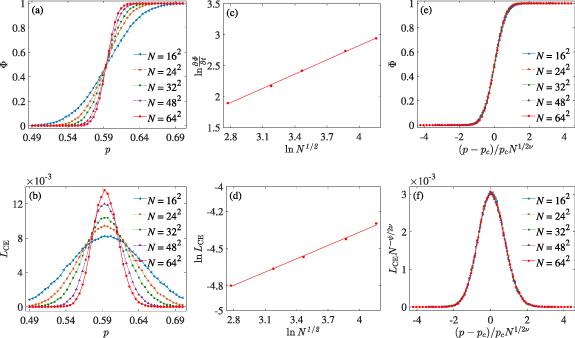
Figure 1. Prediction results using CNN on the square lattices for site percolation, labeled based on the relative size of the largest connected cluster. (a) Phase transition probability $\Phi$ as a function of the lattice occupation probability $p$. (b) Cross-entropy $L_{\mathrm{CE}}$ as a function of the lattice occupation probability $p$. (c), (d) Logarithmic curves of $\partial\Phi/\partial t$ and $L_{\mathrm{CE}}$ as a function of system size $N^{1/2}$. (e), (f) Collapse curves of different system sizes. |
Figure 2 shows the phase transition recognition results of two-dimensional square lattice bond percolation. In figures 2(a) and (b), the phase transition probability curves and the cross-entropy loss curves are presented, respectively. The intersection points of the curves for different system sizes allow the identification of the critical point $p_\mathrm{c} = 0.500(4)$. Figure 2(c) displays the logarithmic relationship between $\partial\Phi/\partial t$ and system size $N^{1/2}$, and the critical exponent $1/\nu$ is obtained by linear fitting as $0.757(23)$. Figure 2(d) shows the logarithmic relationship between $L_{\mathrm{CE}}$ and $N^{1/2}$, and the linear fitting results give the critical exponent $\psi/\nu = 0.468(23)$ for the cross-entropy. Furthermore, based on the obtained critical exponents, a data collapse analysis was performed, as shown in figures 2(e) and (f), where all data points exhibit good scaling collapse behavior. This result indicates that the observable-based labeling strategy can effectively identify the phase transition characteristics of square lattice bond percolation model.
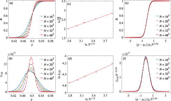
Figure 2. Prediction results using CNN on the square lattices for bond percolation, labeled based on the relative size of the largest connected cluster. (a) Phase transition probability $\Phi$ as a function of the lattice occupation probability $p$. (b) Cross-entropy $L_{\mathrm{CE}}$ as a function of the lattice occupation probability $p$. (c), (d) Logarithmic curves of $\partial\Phi/\partial t$ and $L_{\mathrm{CE}}$ as a function of system size $N^{1/2}$. (e), (f) Collapse curves of different system sizes. |
3.1.2. Site percolation and bond percolation on triangular lattices.
For site and bond percolation on two-dimensional triangular lattices, the dataset construction, sample labeling, model training, and testing procedures were the same as those used for the square-lattice case. Here, we focus only on the settings that differ from the square-lattice models and the corresponding results.
For the site percolation model, Monte Carlo simulations were performed at the theoretical critical point $p_\mathrm{c} = 0.5$ for different system sizes ($N^{1/2} = 16, 24, 32, 48, 64$), with $10^5$ independent samples generated for each size. The mean values of the relative size of the largest connected cluster, $S_{\max}$, at the critical point were 0.2919(3), 0.2717(3), 0.2596(3), 0.2448(3), and 0.2360(3), respectively, and these values were used as the labeling thresholds. The site percolation configurations were again encoded as binary matrices of size $N^{1/2}\times N^{1/2}$. For the bond percolation model, Monte Carlo simulations were carried out at the theoretical critical point $p_\mathrm{c} = 0.3473$ for system sizes $N^{1/2} = 16, 20, 24, 32, 48$, again with $10^5$ independent samples generated for each size. The corresponding mean values of $S_{\max}$ were 0.7294(5), 0.7119(5), 0.6994(4), 0.6783(4), and 0.6502(4), and were used as the labeling thresholds. Unlike the square-lattice bond percolation case, the input configurations were represented as binary matrices of size $3N^{1/2}\times N^{1/2}$ to accommodate the connectivity structure of the triangular lattice, where 0 and 1 denote unoccupied and occupied edges, respectively.
The test intervals of the occupation probability were also adjusted accordingly: 50 occupation probability values were uniformly selected from $[0.356, 0.650]$ for site percolation and from $[0.250, 0.449]$ for bond percolation, with 20 000 configurations generated at each occupation probability. After training, the neural network outputs on the test set yielded the percolation probability curves and the corresponding cross-entropy loss curves for different system sizes, which were used for further analysis and comparison of the phase transition characteristics of the system.
Figure 3 presents the phase transition identification results of two-dimensional triangular lattice site percolation. Among them, figures 3(a) and (b) respectively show the phase transition probability curve and the cross-entropy loss curve. The critical point position $p_\mathrm{c}$ of the system can be identified as $0.500(6)$ from the intersection points of the curves of different system sizes. Figure 3(c) shows the double logarithmic relationship of $\partial \Phi/\partial t$ with system size, and the critical exponent $1/\nu$ is obtained as $0.757(28)$ through linear fitting. Figure 3(d) displays the double logarithmic relationship of $L_{\mathrm{CE}}$ with $N^{1/2}$, and the linear fitting result gives the critical exponent $\psi/\nu$ of cross-entropy as $0.344(8)$. Further, based on the obtained critical exponents, data collapse analysis was conducted, and the results are shown in figures 3(e) and (f). All data points exhibit good scaling collapse behavior. This result indicates that the marking strategy based on the observable can effectively identify the phase transition characteristics of the two-dimensional triangular lattice site percolation model.
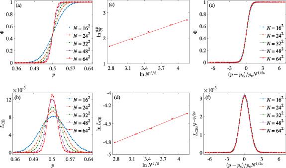
Figure 3. Prediction results using CNN on the triangular lattices for site percolation, labeled based on the relative size of the largest connected cluster. (a) Phase transition probability $\Phi$ as a function of the lattice occupation probability $p$. (b) Cross-entropy $L_{\mathrm{CE}}$ as a function of the lattice occupation probability $p$. (c), (d) Logarithmic curves of $\partial\Phi/\partial t$ and $L_{\mathrm{CE}}$ as a function of system size $N^{1/2}$. (e), (f) Collapse curves of different system sizes. |
Figure 4 presents the phase transition identification results of two-dimensional triangular lattice bond percolation. Among them, figures 4(a) and (b) respectively show the phase transition probability curve and the cross-entropy loss curve. The critical point position $p_\mathrm{c}$ of the system can be identified as $0.348(4)$ from the intersection points of the curves of different system sizes. Figure 4(c) shows the double logarithmic relationship of $\partial \Phi/\partial t$ with system size, and the critical exponent $1/\nu$ is obtained as $0.737(28)$ through linear fitting. Figure 4(d) displays the double logarithmic relationship of $L_{\mathrm{CE}}$ with $N^{1/2}$, and the linear fitting result gives the critical exponent $\psi/\nu$ of cross-entropy as $0.528(18)$. Further, based on the obtained critical exponents, data collapse analysis was conducted, and the results are shown in figures 4(e) and (f). All data points exhibit good scaling collapse behavior. This result indicates that the marking strategy based on the observable can effectively identify the phase transition characteristics of the two-dimensional triangular lattice bond percolation model.
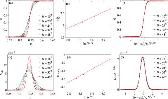
Figure 4. Prediction results using CNN on the triangular lattices for bond percolation, labeled based on the relative size of the largest connected cluster. (a) Phase transition probability $\Phi$ as a function of the lattice occupation probability $p$. (b) Cross-entropy $L_{\mathrm{CE}}$ as a function of the lattice occupation probability $p$. (c), (d) Logarithmic curves of $\partial\Phi/\partial t$ and $L_{\mathrm{CE}}$ as a function of system size $N^{1/2}$. (e), (f) Collapse curves of different system sizes. |
3.1.3. Bond percolation on ER networks.
For the bond percolation model on ER networks, simulations of the $S_{\max}$ were conducted at the theoretical critical point $p_\mathrm{c} = 0.5$ across various system sizes. For each system size, 100 000 independent samples were generated. The resulting average of the $S_{\max}$ at the theoretical critical point for the respective system sizes are as follows: 0.2239(2), 0.1761(2), 0.1397(2), 0.1111(2), and 0.0975(1). In the model training phase, the GCN framework is used. In both the training set and the validation set, 2000 configurations were uniformly selected within the probability range [0, 1]. The test set takes 32 probability values in the [0.03 125, 1] interval, and generates 20 000 configurations for each probability. The sample is marked as follows: if the $S_{\max}$ exceeds the set threshold, it is marked as 1 ; Conversely, it is marked as 0. After the training is completed, the model is used for the classification recognition of the test set, and the training process of GCN is averaged 50 times. Finally, the corresponding curves of the output values of the neural network and the cross-entropy loss curves under the system size $N = 64,128,256,512,768$ are obtained.
Figure 5 presents the phase transition identification results of bond percolation on the ER network. In this figure, figures 5(a) and (b) respectively show phase transition probability curves and the cross-entropy loss curves. The intersection points of the curves corresponding to different system sizes can identify the critical point position $T_\mathrm{c}$ of the system as $ 0.500(31)$. Figure 5(c) shows the double logarithmic relationship of $\partial \Phi/\partial t$ with respect to the system size $N$. Through linear fitting, the critical exponent $1/\nu$ is obtained as $ 0.324(8)$. Figure 5(d) displays the double logarithmic relationship of $L_{\mathrm{CE}}$ with respect to $N$, and the linear fitting result gives the critical exponent ${\psi}/{\nu}$ of the cross-entropy as $0.024(10)$. Further, based on the obtained critical exponents, data collapse analysis was conducted, and the results are shown in figures 5(e) and (f). All data points exhibit good scaling collapse behavior. This result indicates that the labeling strategy based on observable can effectively identify the phase transition characteristics of the ER networks percolation model.
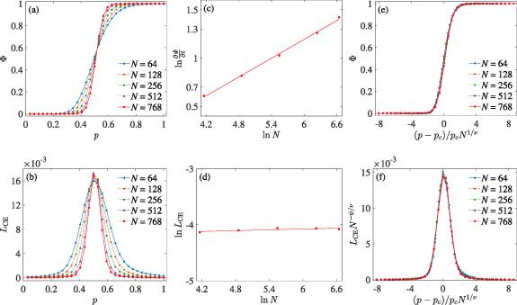
Figure 5. Prediction results using GCN on the ER networks for bond percolation, labeled based on the relative size of the largest connected cluster. (a) Phase transition probability $\Phi$ as a function of the lattice occupation probability $p$. (b) Cross-entropy $L_{\mathrm{CE}}$ as a function of the lattice occupation probability $p$. (c), (d) Logarithmic curves of $\partial \Phi/\partial t$ and $L_{\mathrm{CE}}$ as a function of system size $N$. (e), (f) Collapse curves of different system sizes. |
3.2. Ising models
In the study of the Ising model, we used observable quantities for labeling, selecting magnetization and energy as observables, and analyzed the Ising phase transitions on square and triangular lattices. Magnetization and energy are key physical quantities for describing the system’s phase transition behavior and can reflect the macroscopic state changes near the critical point. Using neural networks, we labeled the system with these physical quantities and studied the Ising phase transition characteristics for different lattice structures. The evolution process of the Ising model was carried out using the Metropolis Monte Carlo algorithm [30]. First, the system was constructed on two-dimensional lattices with periodic boundary conditions. For each temperature, 50 random initializations were performed, and after each initialization, a 2000-step thermalization process was executed to ensure the system reached equilibrium. Then, for each initialization, 2000 configurations were sampled (with a gap of 10 Monte Carlo steps between each configuration), and the magnetization and energy were recorded for each configuration.
3.2.1. Ising model on square lattices.
To further verify the applicability of the observables-based labeling strategy in phase transition recognition, we selected the Ising model on a two-dimensional square lattice as the research object. At different system sizes, the changes in absolute magnetization and energy were simulated at the theoretical critical temperature $T_\mathrm{c} = 2.2692$. For each system size, 10 0000 samples were independently generated. The average absolute magnetization at the critical temperature for different sizes were: 0.7136(6), 0.6943(6), 0.6775(6), 0.6542(6), and 0.6286(5); the average energy were: $-$1.4525(5), $-$1.4457(5), $-$1.4404(4), $-$1.4339(3), and $-$1.4286(2). In the model training stage, a CNN architecture was adopted. The training set was generated by selecting a temperature point every 0.2 within the temperature range [0.5$T_\mathrm{c}$, 1.5$T_\mathrm{c}$], with 1000 configurations generated at each temperature, totaling 114 000 training samples. The validation set was generated by creating 500 configurations at each temperature point, resulting in a total of 57 000 samples. The test set was generated by uniformly selecting 40 temperature points within the range [1.5, 3], with 20 000 configurations generated at each temperature. The samples were labeled based on magnetization and energy. A configuration is labeled as 1 (disordered phase) if its absolute magnetization is below the threshold or its energy is above the threshold. Conversely, it is labeled as 0 (ordered phase) if its absolute magnetization exceeds the threshold or its energy is below the threshold. After training, the CNN model was used to classify and identify phase transitions in the test set. Finally, the phase transition probability curves and cross entropy loss curves for system sizes $N^{1/2}$ = 16, 20, 24, 32, and 48 were obtained.
Figure 6 presents the phase transition identification results of the Ising model on a two-dimensional square lattice, the observable is the magnetization. In this figures 6(a) and (b) respectively show the phase transition probability curves and the cross-entropy loss curves. The intersection points of the output value curves of the neural network under different system sizes can identify the critical temperature position $T_\mathrm{c}$ of the system as $ 2.269(39)$. Figure 6(c) shows the double logarithmic relationship of $\partial \Phi/\partial t$ with respect to the system size $N^{1/2}$. Through linear fitting, the critical exponent $1/\nu$ is obtained as $ 0.950(49)$. Figure 6(d) displays the double logarithmic relationship of $L_{\mathrm{CE}}$ with respect to $N^{1/2}$, and the linear fitting result gives the critical exponent ${\psi}/{\nu}$ of the cross-entropy as $ 0.132(10)$. Furthermore, based on the obtained critical exponents, data collapse analysis was conducted, and the results are shown in figures 6(e) and (f). All data points exhibit good scaling collapse behavior. This result indicates that the labeling strategy based on magnetization can effectively identify the phase transition characteristics of the Ising model on a two-dimensional square lattice.
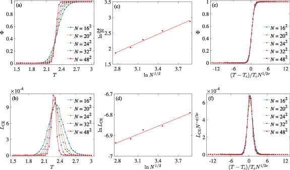
Figure 6. Prediction results using CNN on Ising models of square lattices, with labels based on magnetization. (a) Phase transition probability $\Phi$ as a function of the temperature $T$. (b) Cross-entropy $L_{\mathrm{CE}}$ as a function of the temperature $T$. (c), (d) Logarithmic curves of $\partial \Phi/\partial t$ and $L_{\mathrm{CE}}$ as a function of system size $N^{1/2}$. (e), (f) Collapse curves of different system sizes. |
Figure 7 presents the phase transition identification results of the Ising model on a two-dimensional square lattice, the observable is the energy. In this figures 7(a) and (b) respectively show the phase transition probability curves and the cross-entropy loss curves. The intersection points of the output value curves of the neural network under different system sizes can identify the critical temperature position $T_\mathrm{c}$ of the system as $ 2.269(39)$. Figure 7(c) shows the double logarithmic relationship of $\partial \Phi/\partial t$ with respect to the system size $N^{1/2}$. Through linear fitting, the critical exponent $1/\nu$ is obtained as $ 0.965(33)$. Figure 7(d) displays the double logarithmic relationship of $L_{\mathrm{CE}}$ with respect to $N^{1/2}$, and the linear fitting result gives the critical exponent ${\psi}/{\nu}$ of the cross-entropy as $ 0.493(18)$. Furthermore, based on the obtained critical exponents, data collapse analysis was conducted, and the results are shown in figures 7(e) and (f). All data points exhibit good scaling collapse behavior. This result indicates that the labeling strategy based on energy can effectively identify the phase transition characteristics of the Ising model on two-dimensional square lattices.
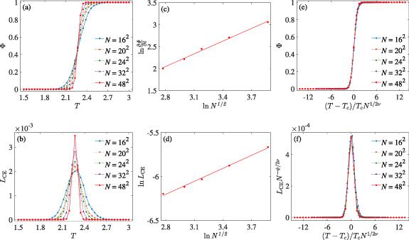
Figure 7. Prediction results using CNN on Ising models of square lattices, with labels based on energy. (a) Phase transition probability $\Phi$ as a function of the temperature $T$. (b) Cross-entropy $L_{\mathrm{CE}}$ as a function of the temperature $T$. (c), (d) Logarithmic curves of $\partial \Phi/\partial t$ and $L_{\mathrm{CE}}$ as a function of system size $N^{1/2}$. (e), (f) Collapse curves of different system sizes. |
3.2.2. Ising model on triangular lattices.
Next, we selected the two-dimensional triangular lattice Ising model as the research object, focusing on two observables: magnetization and energy. We performed Monte Carlo simulations at the theoretical critical temperature $T_\mathrm{c} = 3.6410$ for different system sizes, generating $10^5$ independent samples for each size. And the average absolute magnetization and energy at the theoretical critical temperature was calculated and used as the labeling threshold. The results showed that the average absolute magnetization at the critical temperature for the different sizes was 0.4306(6), 0.4191(6), 0.4078(6), and 0.3947(6), respectively, while the corresponding average energy values were $-1.6284(4)$, $-1.6845(4)$, $-1.7241(4)$, and $-1.7782(4)$. During the model training phase, a CNN architecture was employed. The training set samples were taken from the temperature interval [0.5$T_\mathrm{c}$, 1.5$T_\mathrm{c}$], with temperature points selected at intervals of 0.2. At each temperature, 1000 configurations were generated, resulting in a total of 114 000 training samples. The validation set consisted of 500 configurations generated at the same temperature points, totaling 57 000 samples. The test set was constructed by uniformly selecting 40 temperature points within the interval [2,6], with 20 000 configurations generated at each temperature. After training, the trained CNN model was used to classify phase transitions for the test set samples. Finally, phase transition probability curves and the corresponding cross-entropy loss curves were obtained for system sizes $N^{1/2} = 16, 20, 24, 32$.
Figures 8 and 9 present the phase transition identification results for the two-dimensional triangular lattice Ising model based on magnetization and energy labeling, respectively. Specifically, figures 8(a), 9(a) and 8(b), 9(b) show the phase transition probability curves and cross-entropy loss curves of the system, respectively. By extracting the intersection points of the phase transition probability curves at different system sizes, the critical temperature of the system is determined to be $ T_\mathrm{c} = 3.641(103) $. To obtain the critical exponents, we further analyzed the finite-size scaling behavior. Figures 8(c) and 9(c) show the double logarithmic relationship between $\partial \Phi/\partial t$ and the system size $N^{1/2}$. Linear fitting yields the critical exponent $1/\nu = 0.925(77)$ for magnetization-based labeling and $ 1/\nu = 0.971(21)$ for energy-based labeling. Meanwhile, figures 8(d) and 9(d) display the double logarithmic relationship between the cross-entropy $L_{\mathrm{CE}}$ and $N^{1/2}$. Linear fitting gives the critical exponent $\psi/\nu $ for energy-based labeling as 0.273(43). Based on the above critical exponents, we performed a data collapse analysis, and the results are shown in figures 8(e), (f) and 9(e), (f), respectively. Comparison reveals that the critical exponents obtained from energy-based labeling are closer to the theoretical values, and the data collapse effect is satisfactory. In contrast, the collapse result based on magnetization-based labeling shows significant deviation.
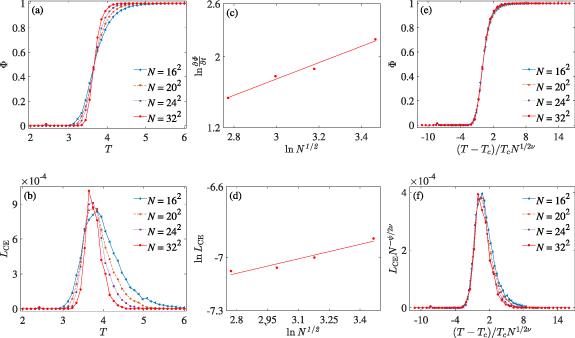
Figure 8. Prediction results using CNN on Ising models of triangular lattices, with labels based on magnetization. (a) Phase transition probability $\Phi$ as a function of the temperature $T$. (b) Cross-entropy $L_{\mathrm{CE}}$ as a function of the temperature $T$. (c), (d) Logarithmic curves of $\partial \Phi/\partial t$ and $L_{\mathrm{CE}}$ as a function of system size $N^{1/2}$. (e), (f) Collapse curves of different system sizes. |
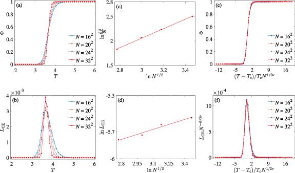
Figure 9. Prediction results using CNN on Ising models of triangular lattices, with labels based on energy. (a) Phase transition probability $\Phi$ as a function of the temperature $T$. (b) Cross-entropy $L_{\mathrm{CE}}$ as a function of the temperature $T$. (c), (d) Logarithmic curves of $\partial \Phi/\partial t$ and $L_{\mathrm{CE}}$ as a function of system size $N^{1/2}$. (e), (f) Collapse curves of different system sizes. |
In the triangular-lattice Ising model, energy-based supervised labeling exhibits superior classification performance and a stronger capacity to characterize critical behavior than magnetization-based labeling. This advantage likely arises from the combined effects of order-parameter fluctuations and lattice geometry. Although magnetization directly captures the spontaneous symmetry breaking of the system, its statistical stability becomes relatively weak in the critical region for finite-size systems due to strong thermal fluctuations. In particular, above $T_\mathrm{c}$, the absolute magnetization rapidly decays to nearly zero, which significantly reduces its ability to discriminate samples in the vicinity of the phase transition. By contrast, the energy reflects the overall local correlations determined by nearest-neighbor interactions, is insensitive to global spin inversion, and varies more smoothly with temperature. It therefore possesses better stability and separability near criticality. Furthermore, the triangular lattice has a larger coordination number, $z = 6$, allowing the energy to incorporate richer local correlation information and thus to characterize microscopic configurations more robustly.
Table 1 summarizes the research results of the labeling method based on observables in two-dimensional square lattices, two-dimensional triangular lattices, ER random networks, and two-dimensional square lattices and two-dimensional triangular lattices Ising models. For the percolation models, the relative size of the largest connected cluster is selected as the observable, while for the Ising models, the magnetization intensity and energy are selected as the observables. It can be seen that this method not only can identify the critical point positions of each system, but also can obtain critical exponents consistent with the theory through fitting. Moreover, the data collapse analysis indicates that the results of each system all exhibit good scaling collapse characteristics. The above results verify the universality and effectiveness of the labeling strategy centered on observables in different types of phase transition systems. Note that for cases with unsatisfactory data collapse, we consider that the corresponding scaling relation has not been established, and the relevant exponents are denoted by ‘$-$’ in table 1.
Table 1. Measurements of critical points and critical exponents ($1/\nu, \psi/\nu$) across different models. The results are categorized into those based on the critical point and those based on observables. |
| Model | Critical point | Based on critical point | Based on observables | ||
|---|---|---|---|---|---|
| $1/\nu$ | $\psi/\nu$ | $1/\nu$ | $\psi/\nu$ | ||
| Site percolation(SL) | $0.593(4)$ | $0.763(20)$ | $0.261(47)$ | $0.767(14)$ | $0.358(10)$ |
| Site percolation(TL) | $0.500(6)$ | $0.762(26)$ | $0.265(15)$ | $0.757(28)$ | $0.344(8)$ |
| Bond percolation(SL) | $0.500(4)$ | $0.737(30)$ | $0.191(12)$ | $0.757(23)$ | $0.468(23)$ |
| Bond percolation(TL) | $0.348(4)$ | $0.761(17)$ | $0.294(49)$ | $0.737(28)$ | $0.528(18)$ |
| Bond percolation(ER) | $0.500(31)$ | $0.309(26)$ | $0.104(8)$ | $0.324(8)$ | $0.024(10)$ |
| Ising-M (SL) | $2.269(39)$ | $0.962(28)$ | $0.019(28)$ | $0.950(49)$ | $0.132(10)$ |
| Ising-E (SL) | $2.269(39)$ | $0.962(28)$ | $0.019(28)$ | $0.965(33)$ | $0.493(18)$ |
| Ising-M (TL) | $3.641(103)$ | $0.926(43)$ | $-$ | $0.925(77)$ | $-$ |
| Ising-E (TL) | $3.641(103)$ | $0.926(43)$ | $-$ | $0.971(21)$ | $0.369(43)$ |
3.3. Comparison with the critical-point-based labeling strategy
In this section, we compare the observable-based labeling method with the traditional critical-point-based labeling strategy. Specifically, we present the comparison results between critical-point labeling and observable-based labeling using the relative size of the largest connected cluster (in the percolation model) and magnetization and energy (in the Ising model) as observables.
As shown in figure 10, for the site percolation model on a two-dimensional square lattice, figure 10(a) demonstrates the labeling method based on the critical point. In this figure, $y_1$ and $y_2$ represent the true label probabilities for non-percolating and percolating configurations, respectively, based on the critical point, while $\hat{y}_1$ and $\hat{y}_2$ represent the corresponding predicted probabilities output by the neural network. It can be observed that there is a significant difference between the true label values and the neural network’s predicted probabilities. Figure 10(b) shows the labeling method based on the relative size of the largest connected cluster. Compared to the critical-point-based labeling, this method shows a closer alignment between the true label values and the predicted probabilities from the neural network. Furthermore, we compare the cross-entropy output by the neural network for the two labeling methods, as shown in figure 10(c). The results indicate that near the theoretical critical point, the cross-entropy obtained from the labeling based on the largest connected cluster is significantly lower than that from the critical-point-based labeling.
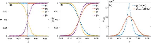
Figure 10. Comparison of labeling methods based on the relative size of the largest connected cluster and based on the critical point for site percolation on a two-dimensional square lattice, with system size $N^{1/2} = 32$. (a) Comparison between true label values and neural network predictions when labeling is based on the critical point. (b) Comparison between true label values and neural network predictions when labeling is based on the relative size of the largest connected cluster. (c) Comparison of the cross-entropy loss of neural network predictions between labeling based on the critical point and labeling based on the relative size of the largest connected cluster. |
For the Ising model on a two-dimensional square lattice, we also conducted the same comparison, as shown in figure 11. Figure 11(a) demonstrates the labeling method based on the critical temperature. In this case, $y_1$ and $y_2$ represent the true label probabilities for the ordered phase and disordered phase, respectively, based on the critical temperature, while $\hat{y}_1$ and $\hat{y}_2$ represent the corresponding predicted probabilities output by the neural network. As in the percolation model, there is a noticeable difference between the true label values and the neural network’s predicted probabilities. Figure 11(b) and (c) provide the comparison results for labeling based on magnetization and energy, respectively. It can be seen that for these two observable-based labeling methods, the true label values and the neural network’s predicted values exhibit much higher consistency. We then further compared the cross-entropy output by the neural network for all three labeling methods in figure 11(d). The results show that at any temperature, the cross-entropy for the labeling based on magnetization and energy is significantly lower than that for the critical temperature-based labeling.
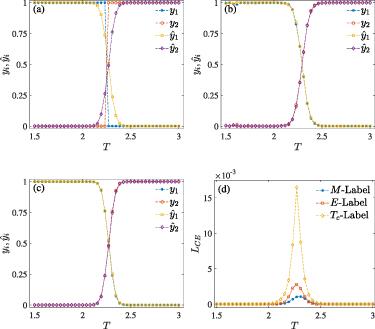


Figure 11. Comparison of labeling methods based on critical temperature, magnetization, and energy for the Ising model on a two-dimensional square lattice, with system size $N^{1/2} = 32$. (a) Comparison between true label values and neural network predictions when labeling is based on the critical temperature. (b) Comparison between true label values and neural network predictions when labeling is based on magnetization. (c) Comparison between true label values and neural network predictions when labeling is based on energy. (d) Comparison of the cross-entropy loss of neural network predictions among the three labeling methods. |
Therefore, the observable-based labeling method demonstrates higher consistency and lower cross-entropy compared to the traditional critical-point-based labeling method. Our experimental results show that the observable-based labeling strategy not only effectively identifies critical points and phase transition properties, but also handles finite-size effects and thermal fluctuations better, thus demonstrating greater stability and accuracy across multiple physical models.
4. Conclusions
This paper introduces a novel labeling strategy grounded in observable quantities for the identification of phase transitions and the analysis of critical properties. In the percolation model, the observable is the relative size of the largest connected cluster, while in the Ising model, the observables are the magnetization and energy. The research results in both models demonstrate that this method can stably identify critical points across different types of phase transitions. By employing finite-size scaling analysis, the method yields critical exponents consistent with theoretical values, proving its universality and reliability across these categories. It demonstrates that observable quantities can not only characterize the macroscopic ordering of the system but also serve as effective machine learning labels, providing a physically interpretable basis for phase transition identification. Compared with traditional labeling methods, this approach offers stronger transferability and physical consistency. Furthermore, the value of the critical exponent $\nu$ obtained through this method can serve as a criterion to determine the universality class of the phase transition, while other related physical properties remain to be further explored. Future research can extend this method to other complex systems, such as the Kosterlitz–Thouless transition and synchronization transition, to further verify its versatility and effectiveness.
It should be noted that the labeling strategy proposed in this paper still references the known theoretical critical point during the threshold construction phase. For entirely new systems where the critical point is completely unknown, the applicability of this method can be extended by combining it with existing critical point localization schemes. First, the ‘learning by confusion’ method [31], which does not rely on prior knowledge of the order parameter, is employed to obtain a preliminary estimate of the critical point location by exploiting the characteristic peaks of the classification accuracy curve in parameter space. After obtaining a rough estimate of the critical point, the observable-based labeling strategy proposed in this paper is introduced. Configurations are simulated near this estimate, and the statistical mean of the observable is extracted to serve as the classification threshold, after which a supervised learning model is trained. We find by comparison that, even under the same candidate critical point, the test accuracy of a classifier constructed using observable-based labeling (such as magnetization or energy) is significantly higher than that achieved by binary labeling directly based on the critical temperature.