

1. Introduction
The spin–orbit coupling (SOC) in ultracold atoms not only alters the dispersion to induce exotic phases (such as the stripe phase and magnetized phase) in boson systems [1–3], but also generates new states of matter in Fermi systems, such as topological superfluids [4–7] and the topological Fulde–Ferrell–Larkin–Ovchinnikov phase [8–11]. Novel quasiparticles of interest in condensed matter physics can also be produced, including Majorana fermions [12–15] and Weyl fermions [16–18]. Experimentally, Raman-type SOC is realized by employing a pair of counter-propagating Raman lasers to dress two atomic spin states [19–29] and is an equal-weight combination of Rashba and Dresselhaus SOCs. For Raman-type SOC, the spin is coupled to the motion of atoms along only one spatial direction, leading to anisotropic dynamical excitations. Recently, we studied the dynamical excitations of a one-dimensional (1D) Raman-type SOC Fermi superfluid and analyzed its primary dynamical characteristics [30]. However, anisotropic behavior cannot be continuously demonstrated in a 1D system due to the existence of only two equivalent directions. Consequently, it is worthwhile to study the angular dependence of anisotropic dynamical properties in a two-dimensional (2D) Raman-type SOC Fermi superfluid, particularly in the collective modes.
The full spectrum of dynamical excitations comprises collective modes and single-particle excitations. A collective mode corresponds to the coherent movement of all particles and is often associated with the breaking of a continuous symmetry in the system, whereas single-particle excitations reveal the information of the energy bands. For example, the breaking of $U(1)$ symmetry in a neutral superfluid gives rise to a gapless Goldstone mode [31, 32]. These dynamical excitations can be investigated through the dynamical structure factors [33–40]. As a two-body correlation observable quantity, the density dynamical structure factor can be directly measured in condensed matter physics through two-photon Bragg spectroscopy in Fermi atomic gases or inelastic neutron-scattering experiments in condensed matter physics [41–49]. Furthermore, several numerical methods have been developed to simulate the density dynamical structure factor [50–54]. Generally, collective modes are studied in the small momentum transfer regime, while the large momentum transfer regime reflects the properties of single-particle excitations.
Theoretically, the dynamical excitations of Fermi gases without SOC have been extensively studied. For SOC Fermi gases, however, only a few studies have discussed dynamical excitations [55–59] due to the complexity of multi-band effects. Consequently, more systematic investigations are necessary. In particular, most research on dynamical excitations has focused on Rashba-type SOC systems [55, 56, 58], which are typically isotropic. Recently, we discussed the dynamical excitations of 2D Fermi superfluids with Rashba-type SOC and found several evolutionary characteristics during the transition from the BCS superfluid to the topological superfluid [56, 60]. Therefore, the anisotropic dynamical behavior induced by SOC is particularly well-suited for investigation in 2D Raman-type systems.
In this paper, by calculating the density dynamical structure factor within the random-phase approximation (RPA), we discuss the effects of Raman-type SOC on the anisotropic dynamical excitations in a 2D Fermi superfluid and investigate the evolution of both collective modes and single-particle excitations across the Lifshitz phase transition.
This paper is organized as follows. In section 2 , starting from the Hamiltonian of a 2D Raman-type Fermi gas, we derive the mean-field Green’s functions using the equations of motion approach; subsequently, the RPA response functions are formulated to obtain the density dynamical structure factor. The main results for the density dynamical structure factor are presented and discussed in section 3 , with a particular focus on the anisotropic collective modes and complex single-particle excitations. Finally, our conclusions are summarized in section 4 . Technical details of the RPA calculations are provided in the appendix.
2. Theoretical framework
In this paper, we consider a 2D two-component SOC superfluid Fermi gas with an $s$-wave contact interaction that can be effectively tuned by the Feshbach resonances [23, 61, 62]. Interestingly, a phase transition occurs in this system at an appropriate Raman-type SOC strength. Since the Raman laser is directed along a specific axis, it induces an anisotropic distribution of physical quantities in space. Consequently, this model provides a suitable platform for investigating the anisotropic physical properties of Fermi superfluids. The Hamiltonian of a 2D Raman-type Fermi gas with an $s$-wave contact interaction is given by [15, 63]:
$\begin{align} H& = \sum_{\sigma}\int \mathrm{d}^{2}\boldsymbol{r}C^{\dagger}_{\sigma}\left(\boldsymbol{r}\right)\left[-\frac{\hbar^{2}}{2m}\nabla^{2}-\mu\right]C_{\sigma}\left(\boldsymbol{r}\right),\nonumber\\ &\quad -h\int \mathrm{d}^2\boldsymbol{r} \left[C^{\dagger}_{\uparrow}\left(\boldsymbol{r}\right)\mathrm{e}^{\mathrm{i}2k_{\mathrm{R}}x}C_{\downarrow}\left(\boldsymbol{r}\right)+C^{\dagger}_{\downarrow}\left(\boldsymbol{r}\right)\mathrm{e}^{-\mathrm{i}2k_{\mathrm{R}}x}C_{\uparrow}\left(\boldsymbol{r}\right)\right],\nonumber\\ &\quad +U_{0}\int \mathrm{d}^{2}\boldsymbol{r}C^{\dagger}_{\uparrow}\left(\boldsymbol{r}\right)C^{\dagger}_{\downarrow}\left(\boldsymbol{r}\right)C_{\downarrow}\left(\boldsymbol{r}\right)C_{\uparrow}\left(\boldsymbol{r}\right),\end{align}$
where $C_{\sigma}$ ($C^{\dagger}_{\sigma}$) is the annihilation (creation) operator for the spin-$\sigma$ component, $m$ is the atomic mass, $\mu$ is the chemical potential, $h$ is the Raman SOC strength, $k_{\mathrm{R}}$ is the recoil momentum of the SOC laser beam, and $U_{0} \lt 0$ is the bare interatomic attractive interaction strength. Here and thereafter, we always set $\hbar = k_\mathrm{B} = 1$. We define two normal density operators, $\hat{n}_{1} = C^{\dagger}_{\uparrow}C_{\uparrow}$ and $\hat{n}_{2} = C^{\dagger}_{\downarrow}C_{\downarrow}$, for the spin-up and spin-down components, respectively. In the superfluid state, two additional anomalous density operators related to superfluid pairing are introduced, namely, $\hat{n}_{3} = C_{\downarrow}C_{\uparrow}$ and $\hat{n}_{4} = C^{\dagger}_{\uparrow}C^{\dagger}_{\downarrow}$, which are Hermitian conjugates of each other. Accordingly, cas ${\Delta} = -U_{0}\langle C_{\downarrow}C_{\uparrow} \rangle$. Although ${\Delta}$ is generally complex, its phase can be arbitrarily chosen as a constant and set to zero due to the $U(1)$ symmetry breaking in the superfluid state, i.e. ${\Delta} = {\Delta}^*$.Within the mean-field theory, the four-operator term in the Hamiltonian equation (1 ) can be dealt with, $C^{\dagger}_{\uparrow}C^{\dagger}_{\downarrow}C_{\downarrow}C_{\uparrow} = n_{1}C^{\dagger}_{\downarrow}C_{\downarrow}+n_{2}C^{\dagger}_{\uparrow}C_{\uparrow}+n_{3}C^{\dagger}_{\uparrow}C^{\dagger}_{\downarrow}+n_{4}C_{\downarrow}C_{\uparrow}$. We use the mean value of operator $ \lt \hat{n}_{\sigma} \gt $ to replace the operator $\hat{n}_{\sigma}$ itself, and $ \lt \hat{n}_{\sigma} \gt $ renormalizes the chemical potential. Therefore, the Hamiltonian has a simplified mean-field form in the momentum space as:
$\begin{align}H_{\mathrm{MF}}& = \sum_{\boldsymbol{k},\sigma}\xi_{\boldsymbol{k}}C^{\dagger}_{\boldsymbol{k}\sigma}C_{\boldsymbol{k}\sigma}+\sum_{\boldsymbol{k}}\left({\Delta}^*C_{-\boldsymbol{k}\uparrow}C_{\boldsymbol{k}\downarrow}+{\Delta} C^{\dagger}_{\boldsymbol{k}\downarrow}C^{\dagger}_{-\boldsymbol{k}\uparrow}\right),\nonumber\\ &\quad -h\sum_{\boldsymbol{k}}\left(C^{\dagger}_{{\boldsymbol{k}+\boldsymbol{k}_{\mathrm{R}}}\uparrow}C_{{\boldsymbol{k}-\boldsymbol{k}_{\mathrm{R}}}\downarrow}+C^{\dagger}_{{\boldsymbol{k}-\boldsymbol{k}_{\mathrm{R}}}\downarrow}C_{{\boldsymbol{k}+\boldsymbol{k}_{\mathrm{R}}}\uparrow}\right),\end{align}$
where the single-particle energy is $\xi_{\boldsymbol{k}} = \boldsymbol{k}^{2}/(2m)-\mu$. Now we define the Green’s functions related to the normal particle density, with spin-up one $G_{\uparrow}(\boldsymbol{k},\tau-\tau^{^{^{\prime}}}) = -\langle T_{\tau} C_{{\boldsymbol{k}+\boldsymbol{k}_{\mathrm{R}}}\uparrow}(\tau)C^{\dagger}_{{\boldsymbol{k}+\boldsymbol{k}_{\mathrm{R}}}\uparrow}(\tau^{^{^{\prime}}})\rangle$ and spin-down one $G_{\downarrow}(\boldsymbol{k},\tau-\tau^{^{^{\prime}}}) = -\langle T_{\tau} C_{{\boldsymbol{k}-\boldsymbol{k}_{\mathrm{R}}}\downarrow}(\tau)C^{\dagger}_{{\boldsymbol{k}-\boldsymbol{k}_{\mathrm{R}}}\downarrow}(\tau^{^{^{\prime}}})\rangle$, where $T_{\tau}$ is a $\tau$-ordering operator. Then an anomalous Green’s function with pairing related terms is defined, namely, $\Gamma^{\dagger}(\boldsymbol{k},\tau-\tau^{^{^{\prime}}}) = -\langle T_{\tau} C^{\dagger}_{{-\boldsymbol{k}-\boldsymbol{k}_{\mathrm{R}}}\downarrow}(\tau)C^{\dagger}_{{\boldsymbol{k}+\boldsymbol{k}_{\mathrm{R}}}\uparrow}(\tau^{^{^{\prime}}})\rangle$. Furthermore, three Green’s functions are brought by the SOC effect, including spin-flip one $S^{\dagger}(\boldsymbol{k},\tau-\tau^{^{^{\prime}}}) = -\langle T_{\tau} C_{{\boldsymbol{k}-\boldsymbol{k}_{\mathrm{R}}}\downarrow}(\tau)C^{\dagger}_{{\boldsymbol{k}+\boldsymbol{k}_{\mathrm{R}}}\uparrow}(\tau^{^{^{\prime}}})\rangle$, spin-up triplet pairing one $F_{1}^{\dagger}(\boldsymbol{k},\tau-\tau^{^{^{\prime}}}) = -\langle T_{\tau} C^{\dagger}_{{-\boldsymbol{k}+\boldsymbol{k}_{\mathrm{R}}}\uparrow}(\tau)C^{\dagger}_{{\boldsymbol{k}+\boldsymbol{k}_{\mathrm{R}}}\uparrow}(\tau^{^{^{\prime}}})\rangle$, and spin-down triplet pairing one $F_{2}^{\dagger}(\boldsymbol{k},\tau-\tau^{^{^{\prime}}}) = -\langle T_{\tau} C^{\dagger}_{{-\boldsymbol{k}-\boldsymbol{k}_{\mathrm{R}}}\downarrow}(\tau)C^{\dagger}_{{\boldsymbol{k}-\boldsymbol{k}_{\mathrm{R}}}\downarrow}(\tau^{^{^{\prime}}})\rangle$. Based on the equations of motion of the Green’s functions, we can analytically derive these Green’s functions as: $\begin{align}G_{\uparrow}\left(\boldsymbol{k},\omega\right)& = \sum_{a}\left[\frac{U^{^{\prime} 2}_{a\boldsymbol{k}}}{\omega-E_{a\boldsymbol{k}}}+ \frac{V^{^{\prime} 2}_{a\boldsymbol{k}}}{\omega+E_{a\boldsymbol{k}}}\right],\nonumber\\G_{\downarrow}\left(\boldsymbol{k},\omega\right)& = \sum_{a}\left[\frac{U^2_{a\boldsymbol{k}}}{\omega-E_{a\boldsymbol{k}}}+ \frac{V^2_{a\boldsymbol{k}}}{\omega+E_{a\boldsymbol{k}}}\right],\nonumber\\ \Gamma^{\dagger}\left(\boldsymbol{k},\omega\right)& = \sum_{a}\left[ \alpha_{a\boldsymbol{k}}\left(\frac{1}{\omega+E_{a\boldsymbol{k}}}-\frac{1}{\omega-E_{a\boldsymbol{k}}}\right)\right],\end{align}$
and $\begin{align}S^{\dagger}\left(\boldsymbol{k},\omega\right)& = \sum_{a}\left[\frac{P_{a\boldsymbol{k}}}{\omega-E_{a\boldsymbol{k}}}+ \frac{Q_{a\boldsymbol{k}}}{\omega+E_{a\boldsymbol{k}}}\right],\nonumber\\F^{\dagger}_{1}\left(\boldsymbol{k},\omega\right)& = \sum_{a}\left[\frac{W_{a\boldsymbol{k}}}{\omega-E_{a\boldsymbol{k}}}+ \frac{T_{a\boldsymbol{k}}}{\omega+E_{a\boldsymbol{k}}}\right],\nonumber\\F^{\dagger}_{2}\left(\boldsymbol{k},\omega\right)& = \sum_{a}\left[\frac{T_{a\boldsymbol{k}}}{\omega-E_{a\boldsymbol{k}}}+ \frac{W_{a\boldsymbol{k}}}{\omega+E_{a\boldsymbol{k}}}\right],\end{align}$
where $a(a^{^{\prime}}) = 1,2$, and $a^{^{\prime}}\neq a$.$U^{^{\prime} 2}_{a\boldsymbol{k}} = (\Omega^{^{\prime}}_{a\boldsymbol{k}}+\Xi^{^{\prime}}_{a\boldsymbol{k}})/\Sigma_{a\boldsymbol{k}}$,
$V^{^{\prime} 2}_{a\boldsymbol{k}} = (\Omega^{^{\prime}}_{a\boldsymbol{k}}-\Xi^{^{\prime}}_{a\boldsymbol{k}})/\Sigma_{a\boldsymbol{k}}$,
$U^2_{a\boldsymbol{k}} = (\Omega_{a\boldsymbol{k}}+\Xi_{a\boldsymbol{k}})/\Sigma_{a\boldsymbol{k}}$,
$V^2_{a\boldsymbol{k}} = (\Omega_{a\boldsymbol{k}}-\Xi_{a\boldsymbol{k}})/\Sigma_{a\boldsymbol{k}}$,
$\alpha_{a\boldsymbol{k}} = [E^{2}_{a\boldsymbol{k}}-(\xi^{2}_{\boldsymbol{k}-\boldsymbol{k}_{\mathrm{R}}}+{\Delta}^{2}-h^{2})]{\Delta}/\Sigma_{a\boldsymbol{k}}$,
$P_{a\boldsymbol{k}} = -h[E^{2}_{a\boldsymbol{k}}+(\xi_{\boldsymbol{k}-\boldsymbol{k}_{\mathrm{R}}}+\xi_{\boldsymbol{k}+\boldsymbol{k}_{\mathrm{R}}})E_{a\boldsymbol{k}}+\xi_{\boldsymbol{k}-\boldsymbol{k}_{\mathrm{R}}}\xi_{\boldsymbol{k}+\boldsymbol{k}_{\mathrm{R}}}+{\Delta}^{2}-h^{2}]/\Sigma_{a\boldsymbol{k}}$,
$Q_{a\boldsymbol{k}} = h[E^{2}_{a\boldsymbol{k}}-(\xi_{\boldsymbol{k}-\boldsymbol{k}_{\mathrm{R}}}+\xi_{\boldsymbol{k}+\boldsymbol{k}_{\mathrm{R}}})E_{a\boldsymbol{k}}+\xi_{\boldsymbol{k}-\boldsymbol{k}_{\mathrm{R}}}\xi_{\boldsymbol{k}+\boldsymbol{k}_{\mathrm{R}}}+{\Delta}^{2}-h^{2}]/\Sigma_{a\boldsymbol{k}}$,
$T_{a\boldsymbol{k}} = h{\Delta}(2E_{a\boldsymbol{k}}+\xi_{\boldsymbol{k}-\boldsymbol{k}_{\mathrm{R}}}-\xi_{\boldsymbol{k}+\boldsymbol{k}_{\mathrm{R}}})/\Sigma_{a\boldsymbol{k}}$,
$W_{a\boldsymbol{k}} = h{\Delta}(2E_{a\boldsymbol{k}}-\xi_{\boldsymbol{k}-\boldsymbol{k}_{\mathrm{R}}}+\xi_{\boldsymbol{k}+\boldsymbol{k}_{\mathrm{R}}})/\Sigma_{a\boldsymbol{k}}$,
$\Sigma_{a\boldsymbol{k}} = 2(E^{2}_{a\boldsymbol{k}}-E^{2}_{a^{^{\prime}}\boldsymbol{k}})E_{a\boldsymbol{k}}$,
$\Omega^{^{\prime}}_{a\boldsymbol{k}} = E^{3}_{a\boldsymbol{k}}-(\xi^{2}_{\boldsymbol{k}-\boldsymbol{k}_{\mathrm{R}}}+{\Delta}^{2}+h^{2})E_{a\boldsymbol{k}}$,
$\Xi^{^{\prime}}_{a\boldsymbol{k}} = \xi_{\boldsymbol{k}+\boldsymbol{k}_{\mathrm{R}}}E^{2}_{a\boldsymbol{k}}+\xi_{\boldsymbol{k}-\boldsymbol{k}_{\mathrm{R}}}h^{2}-\xi_{\boldsymbol{k}+\boldsymbol{k}_{\mathrm{R}}}{\Delta}^{2}-\xi^{2}_{\boldsymbol{k}-\boldsymbol{k}_{\mathrm{R}}}\xi_{\boldsymbol{k}+\boldsymbol{k}_{\mathrm{R}}}$,
$\Omega_{a\boldsymbol{k}} = E^{3}_{a\boldsymbol{k}}-(\xi^{2}_{\boldsymbol{k}+\boldsymbol{k}_{\mathrm{R}}}+{\Delta}^{2}+h^{2})E_{a\boldsymbol{k}}$,
$\Xi_{a\boldsymbol{k}} = \xi_{\boldsymbol{k}-\boldsymbol{k}_{\mathrm{R}}}E^{2}_{a\boldsymbol{k}}+\xi_{\boldsymbol{k}+\boldsymbol{k}_{\mathrm{R}}}h^{2}-\xi_{\boldsymbol{k}-\boldsymbol{k}_{\mathrm{R}}}{\Delta}^{2}-\xi^{2}_{\boldsymbol{k}+\boldsymbol{k}_{\mathrm{R}}}\xi_{\boldsymbol{k}-\boldsymbol{k}_{\mathrm{R}}}$.
The quasiparticle spectra
$\begin{align}E_{1\boldsymbol{k}} = \sqrt{\left(\Theta_{\boldsymbol{k}}+\theta_{\boldsymbol{k}}\right)/2},\nonumber\\E_{2\boldsymbol{k}} = \sqrt{\left(\Theta_{\boldsymbol{k}}-\theta_{\boldsymbol{k}}\right)/2},\end{align}$
where $\Theta_{\boldsymbol{k}} = \xi^{2}_{\boldsymbol{k}-\boldsymbol{k}_{\mathrm{R}}}+\xi^{2}_{\boldsymbol{k}+\boldsymbol{k}_{\mathrm{R}}}+2({\Delta}^{2}+h^{2})$, $\theta_{\boldsymbol{k}}$ $ = \sqrt{(\xi^{2}_{\boldsymbol{k}-\boldsymbol{k}_{\mathrm{R}}}-\xi^{2}_{\boldsymbol{k}+\boldsymbol{k}_{\mathrm{R}}})^{2}+4h^{2}(\xi_{\boldsymbol{k}-\boldsymbol{k}_{\mathrm{R}}}+\xi_{\boldsymbol{k}+\boldsymbol{k}_{\mathrm{R}}})^{2}+16{\Delta}^{2}h^{2}}$. The pair parameters ${\Delta}$ and chemical potential $\mu$ are calculated self-consistently by solving the order parameter equation ${\Delta} = -U_{0} \lt C_{\downarrow}C_{\uparrow} \gt $ and the density equation $n = n_{\uparrow}+n_{\downarrow}$, respectively. Then we get two self-consistent equations, $\begin{align}n& = \sum_{\boldsymbol{k}a}\left[\left(U^{^{\prime} 2}_{a\boldsymbol{k}}+U^2_{a\boldsymbol{k}}\right)n_{\mathrm{F}}\left(E_{a\boldsymbol{k}}\right)+\left(V^{^{\prime} 2}_{a\boldsymbol{k}}+V^2_{a\boldsymbol{k}}\right)n_{\mathrm{F}}\left(-E_{a\boldsymbol{k}}\right)\right], \nonumber\\ \frac{1}{U_{0}}& = -\sum_{\boldsymbol{k}}\left[\frac{\alpha_{1\boldsymbol{k}}}{2E_{1\boldsymbol{k}}}\tanh\left(\frac{1}{2}\beta E_{1\boldsymbol{k}}\right)+\frac{\alpha_{2\boldsymbol{k}}}{2E_{2\boldsymbol{k}}}\tanh\left(\frac{1}{2}\beta E_{2\boldsymbol{k}}\right)\right].\nonumber\\ \end{align}$
The parameters ${\Delta}$ and $\mu$ can be obtained for given SOC strength $h$ and an s-wave contact interaction $U_{0}$. To eliminate the divergence of the pairing order parameter equation introduced by the s-wave contact interaction, the bare interaction strength $U_{0}$ should be regularized by [14] $\begin{align} \frac{1}{U_{0}} = -\sum_{\boldsymbol{k}}\frac{1}{2\epsilon_{\boldsymbol{k}}+E_{\mathrm{b}}},\end{align}$
where $E_{\mathrm{b}}$ is magnitude of binding energy and can be expressed through the 2D s-wave scattering length $a_{\mathrm{2D}}$, namely, $E_{\mathrm{b}} = 4\hbar^{2}/(ma_{\mathrm{2D}}^{2}\mathrm{e}^{2\gamma})$, $\gamma\simeq 0.577$ is the Euler’s constant [37, 64]. The $a_{\mathrm{2D}}$ can be tuned by 2D Feshbach resonances [61], then the BEC-BCS crossover in a 2D Fermi gas can be realized. As a result, our calculations are controllable without using any adjustable parameters.In a uniform 2D system with density $n$, we can use Fermi wave vector $k_{\mathrm{F}} = \sqrt{2\pi n}$ and Fermi energy $\varepsilon_{\mathrm{F}} = {k_{\mathrm{F}}}^{2}/(2m)$ as units of momentum and energy. To guarantee the reliability of the results, we take a relatively weak interaction strength $E_{\mathrm{b}} = 0.05\varepsilon_{\mathrm{F}}$. In the entire paper, the recoil momentum is taken as a typical experimental value, $k_{\mathrm{R}}/k_{\mathrm{F}} = 0.75$ [22]. ${\Delta}$ and $\mu$ strongly depend on the SOC strength. Therefore, we plot ${\Delta}$ and $\mu$ as a function of $h$ at $E_{\mathrm{b}} = 0.05\varepsilon_{\mathrm{F}}$ in figure 1. The Lifshitz phase transition point is marked by the critical effective SOC strength $h_{c} = 0.42\varepsilon_{\mathrm{F}}$. With the increase of $h$, the pair parameter ${\Delta}$ decreases slowly at low $h$, then decreases quickly at larger $h \gt h_{c}$, while the chemical potential $\mu$ is almost a constant until it reaches the highest value at $h_{c}$, then decreases when $h \gt h_{c}$. By calculating the spectral function, we can obtain the information of the electronic structure, particularly in Fermi surface. When $h = 0$, the Fermi surface is gapped by the pairing gap. As $h$ increases, the excitation gap decreases and then disappears. When $h$ is enough large, the energy bands cross the Fermi energy, leading to the appearance of Fermi surface. With $h$ further increases, the Fermi surface exhibits different topological structure, i.e. the Lifshitz phase transition happens.
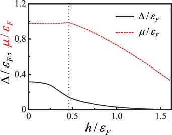
Figure 1. The order parameter ${\Delta}$ (black solid line) and chemical potential $\mu$ (red dashed line) as a function of SOC strength $h$. The critical effective SOC strength is around $h_{c} = 0.42\varepsilon_{\mathrm{F}}$. |
All density related dynamical excitations can be investigated by the density dynamical structure factor, which is related to the density response function $\chi_{D} = \chi_{11}+\chi_{22}+\chi_{12}+\chi_{21}$ by
$\begin{equation}S\left(\boldsymbol{q},{\omega}\right) = -\frac{1}{\pi}\frac{1}{1-\mathrm{e}^{-\omega/T}}\mathrm{Im}\,\chi_{D}\left(\boldsymbol{q},\mathrm{i}\omega_{n}\to \omega+\mathrm{i}\delta\right),\end{equation}$
where $q$ and $\omega$ are the transferred momentum and energy, respectively. $\delta$ is a small positive number, we set $\delta = 0.001$ in the entire paper. The response function $\chi$ can be obtained by the RPA. More details of $\chi$ under the RPA theory are presented in appendix.The RPA theory is widely used to study the dynamical excitation in condensed matter physics and ultra-cold atoms [65–68], and it even obtains quantitatively consistent results in three-dimensional (3D) Fermi superfluids when compared with two-photon Bragg spectroscopy [35, 45, 69]. In particular, for 2D Fermi atoms, the qualitative consistent results with the quantum Monte Carlo calculations are exhibited [37, 39, 51]. We therefore expect that our theoretical calculations are reliable for a 2D Fermi gas in the weak-coupling regimes.
3. SOC dependence of the dynamical excitations
The SOC can significantly modify the chemical potential, the pairing gap, and the quasiparticle spectra, thereby altering the dynamical excitations of the system. In this section, we investigate the SOC dependence of these excitations by calculating the density dynamical structure factor of 2D Fermi gases with Raman-type SOC. Since collective phonon modes typically emerge in a small transferred momentum region, we focus on the evolution of dynamical excitations under SOC at small $q$. In figure 2, we present the color maps of the density dynamical structure factor $S(q, \omega)$ from $q = 0$ to $q = 1k_{\mathrm{F}}$ for SOC strengths of (a) $h = 0$ and (b) $h = 0.45\varepsilon_{\mathrm{F}}$.
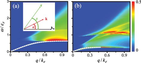
Figure 2. Color maps of the density dynamical structure factor $S(q, \omega)$ from $q = 0$ to $q = 1k_{\mathrm{F}}$ at a weak interaction strength $E_{\mathrm{b}} = 0.05\varepsilon_{\mathrm{F}}$ for SOC strengths (a) $h = 0$ and (b) $h = 0.45\varepsilon_{\mathrm{F}}$. The white dashed lines indicate the collective mode dispersions obtained from the RPA poles. Inset: momentum vectors $\boldsymbol{k}$, ${\boldsymbol{k}_{\mathrm{R}}}$ (recoil momentum), and the angles $\varphi$ (between $\boldsymbol{k}$ and ${\boldsymbol{k}_{\mathrm{R}}}$), $\theta$ (between the transferred momentum $\boldsymbol{q}$ and ${\boldsymbol{k}_{\mathrm{R}}}$). $\varphi$ is integrated out during the integration process. |
For $h = 0$ (in the absence of SOC), a gapless collective mode, characterized by a sharp $\delta$-like peak, emerges and exhibits a nearly linear dispersion ($\omega \propto q$) in the small transferred momentum region. This collective mode is identified as the Goldstone phonon mode, arising from the spontaneous breaking of $U(1)$ gauge symmetry of pairing gap in the superfluid state. The single-particle excitations appear when the transferred energy exceeds a horizontal threshold, $\omega = 2{\Delta} = 0.63\varepsilon_{\mathrm{F}}$, which represents the minimum energy required to break a Cooper pair. In contrast, for $h = 0.45\varepsilon_{\mathrm{F}}$, both the phonon mode and the single-particle excitations deviate significantly from the zero-field results, indicating that the dynamical excitations are highly sensitive to the SOC strength and exhibit a much more complex structure than those in the $h = 0$ case. Detailed analyses of these features are provided in the following subsections. Furthermore, the collective phonon mode corresponds to the poles of the RPA response function $\chi$, determined by the zeros of the denominator: $\mathrm{Re}\,[\hat{1}-\chi^{0}(\boldsymbol{q}, \mathrm{i}\omega_{n})U_{0}M_{\mathrm{I}}] = 0$. The numerical solutions to this equation are indicated by the white dashed lines in figure 2.
3.1. Anisotropic phonon mode
The sound velocity is defined by the slope of the phonon mode in the limit $q \to 0$, namely, $c_{\mathrm{s}} = \omega/q$. In our calculations, $c_{\mathrm{s}}$ is extracted by fitting the position of the $\delta$-like peak in $S(\boldsymbol{q}, \omega)$ at a small transferred momentum ($q = 0.1k_{\mathrm{F}}$). For a 2D non-interacting Fermi gas, the analytical sound velocity is $c_{\mathrm{s}} = v_{\mathrm{F}}/\sqrt{2} \approx 0.707v_{\mathrm{F}}$. As shown in figure 2(a), the calculated sound velocity is $c_{\mathrm{s}} = 0.714v_{\mathrm{F}}$, which is in close agreement with the ideal gas result. To elucidate the angular anisotropy of the phonon mode, we plot $S(\boldsymbol{q} = 0.1k_{\mathrm{F}}, \omega)$ as a function of $\omega$ for $\theta/\pi = 0$ (black solid line), $0.25$ (red dashed line), and $0.5$ (blue dotted line) in figure 3(a). The corresponding sound velocity $c_{\mathrm{s}}$ as a function of the angle $\theta$ is presented in figure 3(b).
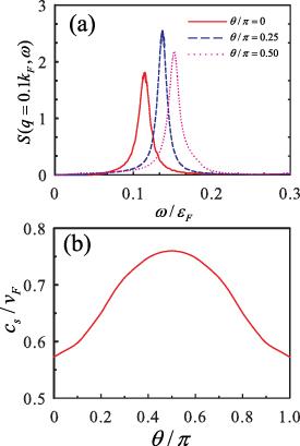
Figure 3. (a) $S(\boldsymbol{q} = 0.1k_{\mathrm{F}}, \omega)$ as a function of $\omega$ for $\theta/\pi = 0$ (black solid line), $0.25$ (red dashed line), and $0.5$ (blue dotted line). (b) Extracted sound velocity $c_{\mathrm{s}}$ versus the angle $\theta$ for $h = 0.45\varepsilon_{\mathrm{F}}$ and $E_{\mathrm{b}} = 0.05\varepsilon_{\mathrm{F}}$. |
The phonon mode exhibits a significant angular dependence, where the position of the sharp resonance peak shifts toward higher energies as $\theta$ increases from $0$ to $0.5\pi$. For instance, the sound velocity at $\theta/\pi = 0$ ($c_{\mathrm{s}} = 0.57v_{\mathrm{F}}$) is notably smaller than that at $\theta/\pi = 0.5$ ($c_{\mathrm{s}} = 0.76v_{\mathrm{F}}$). Furthermore, comparing figures 2(a) and (b), the phonon mode at $h = 0.45\varepsilon_{\mathrm{F}}$ possesses a larger spectral width than the $h = 0$ case. This broadening is attributed to the intense competition between the phonon mode and the gapless single-particle excitations.
3.2. SOC-dependent sound velocity
To further characterize the phonon mode, we calculate the sound velocity as a function of the SOC strength $h$, as shown in figure 4. Our results demonstrate that the sound velocity exhibits a non-monotonic dependence on the SOC strength. Specifically, $c_{\mathrm{s}}$ initially decreases with increasing $h$ and subsequently increases once $h$ exceeds the phase transition point, which is different from the case in 2D Rashba-type SOC Fermi superfluid [56]. The SOC dependence of the sound speed under a weak interaction can be understood qualitatively [70]. The sound speed is closely related to the root-mean-square Fermi velocity, namely, $c_{\mathrm{s}}\propto\sqrt{\langle v_{\mathrm{F}}^{2}\rangle}$, where $v_{\mathrm{F}}$ the Fermi velocity. When $h = 0$ (without SOC), the Fermi velocity $v_{\mathrm{F}} = {\partial \xi_{\boldsymbol{k}}}/{\partial \boldsymbol{k}}|_{\boldsymbol{k} = [k_{\mathrm{F}x},k_{\mathrm{F}y}]}$ is constant. However, when the SOC strength $h \gt 0$, the energy spectra (equation (5 )) become complex, then the Fermi velocity depends on $k_{\mathrm{R}}$ and $h$. Consequently, the sound speed also depends on $k_{\mathrm{R}}$ and $h$.
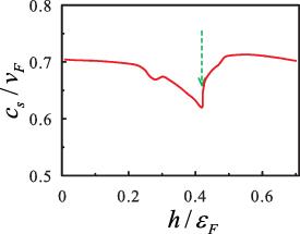
Figure 4. Sound velocity $c_{\mathrm{s}}$ as a function of the SOC strength $h$. The green arrow indicates the critical point of the Lifshitz phase transition. |
3.3. Anisotropic single-particle excitations
In the large transferred energy regime, the dynamical excitations of the system are dominated by single-particle excitations. Most of these excitations are associated with pair-breaking processes, where the absorption of sufficient energy causes Cooper pairs to dissociate into free fermionic atoms. Due to the presence of SOC, the single-particle excitations exhibit a more intricate structure compared to the case without SOC, where a uniform horizontal threshold appears at $\omega = 2{\Delta}$. Consequently, it is essential to investigate the threshold energy required to break a Cooper pair under the SOC effect. The two atoms forming a Cooper pair can originate from the two branches of the quasiparticle spectra, $E_{1\boldsymbol{k}}$ and $E_{2\boldsymbol{k}}$, giving rise to four distinct pair-breaking mechanisms: $\{11\}\rightarrow E_{1(\boldsymbol{k}+\boldsymbol{q})}+E_{1\boldsymbol{k}}$, $\{12\}\rightarrow E_{1(\boldsymbol{k}+\boldsymbol{q})}+E_{2\boldsymbol{k}}$, $\{21\}\rightarrow E_{2(\boldsymbol{k}+\boldsymbol{q})}+E_{1\boldsymbol{k}}$, and $\{22\}\rightarrow E_{2(\boldsymbol{k}+\boldsymbol{q})}+E_{2\boldsymbol{k}}$. Since the $\{12\}$- and $\{21\}$-type excitations overlap, only three types of pair-breaking thresholds are displayed. These thresholds, representing the minima of the pair-breaking energies, typically manifest as the edge curves of the dynamical structure factor shown in figure 2(b).
In figure 5, the minimum energies of three pair-breaking excitations are shown under different SOC strength for (a) $h = 0.2\varepsilon_{\mathrm{F}}$, (b) $h = 0.45\varepsilon_{\mathrm{F}}$. The results show that the minimum energies required for these three pair-breaking excitations depends on the SOC strength, particularly for the $\{22\}$-type excitations (magenta dotted line). At $h = 0.2\varepsilon_{\mathrm{F}}$, a distinct excitation gap is observed and decreases as $h$ increases. The excitation gap eventually vanishes at $h = 0.45\varepsilon_{\mathrm{F}}$, indicating that the $\{22\}$-type excitations become gapless. Moreover, the blue dashed line (the red solid line) denotes the 12-type (11-type) minimum energy. These excitations remain gapped, reflecting the coupling between spin and orbital degrees of freedom. Generally, the signal from $\{11\}$-type excitations is the weakest, as will be further shown in figure 6.
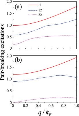
Figure 5. Three types of threshold energies for pair-breaking excitations at different momenta for (a) $h = 0.2\varepsilon_{\mathrm{F}}$ and (b) $h = 0.45\varepsilon_{\mathrm{F}}$. Red solid line: $\min[\{11\}]$ ($\min[E_{1(\boldsymbol{k}+\boldsymbol{q})}+E_{1\boldsymbol{k}}]$); blue dotted line: $\min[\{12\}]$ ($\min[E_{1(\boldsymbol{k}+\boldsymbol{q})}+E_{2\boldsymbol{k}}]$); magenta dotted line: $\min[\{22\}]$ ($\min[E_{2(\boldsymbol{k}+\boldsymbol{q})}+E_{2\boldsymbol{k}}]$). |
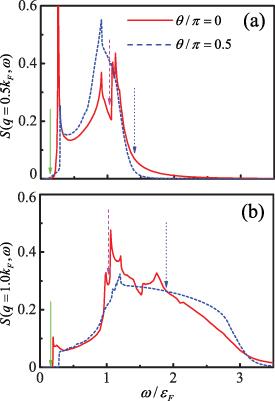


Figure 6. Dynamic structure factor $S(q, \omega)$ at (a) $q = 0.5k_{\mathrm{F}}$ and (b) $q = 1.0k_{\mathrm{F}}$ for $\theta/\pi = 0$ (red solid line) and $\theta/\pi = 0.5$ (blue dashed line) with $h = 0.45\varepsilon_{\mathrm{F}}$. For $\theta/\pi = 0$, the green solid, magenta dashed, and blue dotted arrows indicate the threshold energies for $\{22\}$-, $\{12\}$-, and $\{11\}$-type excitations, respectively. |
To better understand the energy and momentum dependencies of the anisotropic dynamical excitations, we calculate the dynamical structure factor at several representative transferred momenta. In figure 6, we plot $S(q, \omega)$ as a function of $\omega$ at the transferred momenta (a) $q = 0.5k_{\mathrm{F}}$ and (b) $q = 1.0k_{\mathrm{F}}$ for $\theta/\pi = 0$ (red solid line), and $\theta/\pi = 0.5$ (blue dashed line) with $h = 0.45\varepsilon_{\mathrm{F}}$, respectively. Along the $\theta/\pi = 0$ direction, the threshold energies for $\{22\}$-, $\{12\}$- (or $\{21\}$-), and $\{11\}$-type excitations are indicated by green solid, magenta dashed, and blue dotted arrows, respectively.
The dynamical excitations exhibit an anisotropic behavior under different $\theta$, which is attributed to the recoil momentum $k_{\mathrm{R}}$ of the SOC laser beam along the polar axis. At $q = 0.5k_{\mathrm{F}}$, a phonon mode peak appears near $\omega = 0.26\varepsilon_{\mathrm{F}}$ for $\theta/\pi = 0$ and $\omega = 0.29\varepsilon_{\mathrm{F}}$ for $\theta/\pi = 0.5$. Compared with the $\theta/\pi = 0$ case, the peak intensity at $\theta/\pi = 0.5$ is significantly suppressed. Furthermore, at $q = 1.0k_{\mathrm{F}}$, the phonon mode enters the single-particle excitation continuum, leading to intense competition between the single-particle excitations and the phonon mode. Consequently, the phonon peak is suppressed, appearing only as a weak feature at $\theta/\pi = 0$ or disappearing entirely at $\theta/\pi = 0.5$. The strong low-energy single-particle excitations result from the SOC effect, which makes $\{22\}$-type pair-breaking excitations (green solid line) to occur at energies lower than the phonon mode.
4. Summary
Within the framework of RPA theory, we have systematically investigated the dynamical excitations of a 2D Fermi superfluid with Raman-type SOC by calculating the density dynamical structure factor. Our theoretical results demonstrate that the dynamical excitations exhibit an obvious angular anisotropy. Specifically, the sound velocity along the direction of the recoil momentum is lower than that in the perpendicular direction. Under the influence of SOC, the single-particle excitations manifest a complex structure, which can be elucidated through three distinct Cooper-pair-breaking mechanisms. These mechanisms are attributed to the combination of two branches of the quasiparticle spectra. Our predictions provide key insights into the modifications of physical properties induced by Raman-type SOC in fermionic systems.
Appendix. Random phase approximation (RPA) and response functions
In a Fermi superfluid, there are four different densities as mentioned above, namely, $n_{1}$, $n_{2}$, $n_{3}$ and $n_{4}$. The interaction makes these densities coupled with each other. Any fluctuation in each kind of density will influence other densities and generate an obvious density fluctuation of them. Also any weak perturbation potential $V_{\mathrm{pert}}$ will generate density fluctuations $\delta n$, and they are connected with each other by response function $\chi$, namely $\delta n = \chi V_{\mathrm{pert}}$, in the frame of linear response theory. In the mean-field level, the mean-field response function is a $4\times4$ matrix as,
$\begin{align} \chi^{0} = \left[\begin{array}{cccc} \chi_{11}^{0} & \chi_{12}^{0} & \chi_{13}^{0} & \chi_{14}^{0}\\ \chi_{21}^{0} & \chi_{22}^{0} & \chi_{23}^{0} & \chi_{24}^{0}\\ \chi_{31}^{0} & \chi_{32}^{0} & \chi_{33}^{0} & \chi_{34}^{0}\\ \chi_{41}^{0} & \chi_{42}^{0} & \chi_{43}^{0} & \chi_{44}^{0} \end{array}\right],\end{align}$
with $\chi_{ij}^{0}\left(r_{1},r_{2},\tau,0\right) = -\left\langle \hat{n}_{i}\left(r_{1},\tau\right)\hat{n}_{j}\left(r_{2},0\right)\right\rangle $ in coordinate $r$ and imaginary time $\tau$ space. For simple, we use a generalized 4 dimension coordinate $R = \left(r,\tau\right)$ to go on discussion. These 16 matrix elements can be calculated by Wick’s theorem. For simplicity, $\begin{align} \chi_{11}^{0} & = -\left\langle \psi_{\uparrow}^{\dagger}\left(r_{1},\tau\right)\psi_{\uparrow}\left(r_{1},\tau\right)\psi_{\uparrow}^{\dagger}\left(r_{2},0\right)\psi_{\uparrow}\left(r_{2},0\right)\right\rangle, \nonumber\\ & = G_{\uparrow}\left(-R\right)G_{\uparrow}\left(R\right)-F_{1}^{\dagger}\left(-R\right)F_{1}\left(R\right),\end{align}$
similarly we can calculated all rest matrix elements. These 16 matrix elements are determined by the corresponding density-density correlation functions which can be obtained by defining corresponding Green’s functions. In fact, as a result of the symmetry of system, only 10 matrix elements are independent, i.e. $\chi^{0}_{12} = \chi^{0}_{21}$, $\chi^{0}_{33} = \chi^{0}_{44}$, $\chi^{0}_{31} = \chi^{0}_{14}$, $\chi^{0}_{32} = \chi^{0}_{24}$, $\chi^{0}_{41} = \chi^{0}_{13}$, $\chi^{0}_{42} = \chi^{0}_{23}$. Based on the mean-field theory by calculating the corresponding Green’s functions in 2D Fermi gas with Raman-type SOC, we can obtain the correlation functions as: $\begin{align} & \chi^{0}_{11}\left(\boldsymbol{q},\mathrm{i}\omega_{n}\right)\nonumber\\ &\quad = \sum_{\boldsymbol{k},aa^{^{\prime}}}\Big[\left(U^{^{\prime} 2}_{a\boldsymbol{k}}U^{^{\prime} 2}_{a^{^{\prime}}\boldsymbol{k}+\boldsymbol{q}}-W_{a\boldsymbol{k}}W_{a^{^{\prime}}\boldsymbol{k}+\boldsymbol{q}}\right)I_{1}\left(\boldsymbol{k},\boldsymbol{q},\mathrm{i}\omega_{n}\right),\nonumber\\ &\qquad +\left(U^{^{\prime} 2}_{a\boldsymbol{k}}V^{^{\prime} 2}_{a^{^{\prime}}\boldsymbol{k}+\boldsymbol{q}}-W_{a\boldsymbol{k}}T_{a^{^{\prime}}\boldsymbol{k}+\boldsymbol{q}}\right)I_{2}\left(\boldsymbol{k},\boldsymbol{q},\mathrm{i}\omega_{n}\right),\nonumber\\ &\qquad +\left(V^{^{\prime} 2}_{a\boldsymbol{k}}U^{^{\prime} 2}_{a^{^{\prime}}\boldsymbol{k}+\boldsymbol{q}}-T_{a\boldsymbol{k}}W_{a^{^{\prime}}\boldsymbol{k}+\boldsymbol{q}}\right)I_{3}\left(\boldsymbol{k},\boldsymbol{q},\mathrm{i}\omega_{n}\right),\nonumber\\ &\qquad +\left(V^{^{\prime} 2}_{a\boldsymbol{k}}V^{^{\prime} 2}_{a^{^{\prime}}\boldsymbol{k}+\boldsymbol{q}}-T_{a\boldsymbol{k}}T_{a^{^{\prime}}\boldsymbol{k}+\boldsymbol{q}}\right)I_{4}\left(\boldsymbol{k},\boldsymbol{q},\mathrm{i}\omega_{n}\right)\Big]\nonumber.\end{align}$
$\begin{align} \chi^{0}_{12}\left(\boldsymbol{q},\mathrm{i}\omega_{n}\right)& = \sum_{\boldsymbol{k},aa^{^{\prime}}}\Big[\left(P_{a\boldsymbol{k}}P_{a^{^{\prime}}\boldsymbol{k}+\boldsymbol{q}}-\alpha_{a\left(-\boldsymbol{k}\right)}\alpha_{a^{^{\prime}}\left(-\boldsymbol{k}-\boldsymbol{q}\right)}\right)I_{1}\left(\boldsymbol{k},\boldsymbol{q},\mathrm{i}\omega_{n}\right),\nonumber\\ &\quad +\left(P_{a\boldsymbol{k}}Q_{a^{^{\prime}}\boldsymbol{k}+\boldsymbol{q}}+\alpha_{a\left(-\boldsymbol{k}\right)}\alpha_{a^{^{\prime}}-\boldsymbol{k}-\boldsymbol{q}}\right)I_{2}\left(\boldsymbol{k},\boldsymbol{q},\mathrm{i}\omega_{n}\right),\nonumber\\ &\quad +\left(Q_{a\boldsymbol{k}}P_{a^{^{\prime}}\boldsymbol{k}+\boldsymbol{q}}+\alpha_{a\left(-\boldsymbol{k}\right)}\alpha_{a^{^{\prime}}-\boldsymbol{k}-\boldsymbol{q}}\right)I_{3}\left(\boldsymbol{k},\boldsymbol{q},\mathrm{i}\omega_{n}\right),\nonumber\\ &\quad +\left(Q_{a\boldsymbol{k}}Q_{a^{^{\prime}}\boldsymbol{k}+\boldsymbol{q}}-\alpha_{a\left(-\boldsymbol{k}\right)}\alpha_{a^{^{\prime}}-\boldsymbol{k}-\boldsymbol{q}}\right)I_{4}\left(\boldsymbol{k},\boldsymbol{q},\mathrm{i}\omega_{n}\right)\Big]\nonumber.\end{align}$
$\begin{align} \chi^{0}_{22}\left(\boldsymbol{q},\mathrm{i}\omega_{n}\right)& = \sum_{\boldsymbol{k} aa^{^{\prime}}}\Big[\left(U^2_{a\boldsymbol{k}}U^2_{a^{^{\prime}}\boldsymbol{k}+\boldsymbol{q}}-T_{a\boldsymbol{k}}T_{a^{^{\prime}}\boldsymbol{k}+\boldsymbol{q}}\right)I_{1}\left(\boldsymbol{k},\boldsymbol{q},\mathrm{i}\omega_{n}\right)\nonumber\\ &\quad +\left(U^2_{a\boldsymbol{k}}V^2_{a^{^{\prime}}\boldsymbol{k}+\boldsymbol{q}}-T_{a\boldsymbol{k}}W_{a^{^{\prime}}\boldsymbol{k}+\boldsymbol{q}}\right)I_{2}\left(\boldsymbol{k},\boldsymbol{q},\mathrm{i}\omega_{n}\right),\nonumber\\ &\quad +\left(V^2_{a\boldsymbol{k}}U^2_{a^{^{\prime}}\boldsymbol{k}+\boldsymbol{q}}-W_{a\boldsymbol{k}}T_{a^{^{\prime}}\boldsymbol{k}+\boldsymbol{q}}\right)I_{3}\left(\boldsymbol{k},\boldsymbol{q},\mathrm{i}\omega_{n}\right),\nonumber\\ &\quad +\left(V^2_{a\boldsymbol{k}}V^2_{a^{^{\prime}}\boldsymbol{k}+\boldsymbol{q}}-W_{a\boldsymbol{k}}W_{a^{^{\prime}}\boldsymbol{k}+\boldsymbol{q}}\right)I_{4}\left(\boldsymbol{k},\boldsymbol{q},\mathrm{i}\omega_{n}\right)\Big]\nonumber.\end{align}$
$\begin{align} \chi^{0}_{13}\left(\boldsymbol{q},\mathrm{i}\omega_{n}\right)& = \sum_{\boldsymbol{k},aa^{^{\prime}}}\Big[\left(W_{a\boldsymbol{k}}P_{a^{^{\prime}}\boldsymbol{k}+\boldsymbol{q}}-U^{^{\prime} 2}_{a\boldsymbol{k}}\alpha_{a^{^{\prime}}\boldsymbol{k}+\boldsymbol{q}}\right)I_{1}\left(\boldsymbol{k},\boldsymbol{q},\mathrm{i}\omega_{n}\right),\nonumber\\ &\quad +\left(P_{a\boldsymbol{k}}T_{a^{^{\prime}}\boldsymbol{k}+\boldsymbol{q}}+U^{^{\prime} 2}_{a\boldsymbol{k}}\alpha_{a^{^{\prime}}\boldsymbol{k}+\boldsymbol{q}}\right)I_{2}\left(\boldsymbol{k}\boldsymbol{q}\mathrm{i}\omega_{n}\right)\nonumber\\ &\quad +\left(Q_{a\boldsymbol{k}}W_{a^{^{\prime}}\boldsymbol{k}+\boldsymbol{q}}-V^{^{\prime} 2}_{a\boldsymbol{k}}\alpha_{a^{^{\prime}}\boldsymbol{k}+\boldsymbol{q}}\right)I_{3}\left(\boldsymbol{k}\boldsymbol{q}\mathrm{i}\omega_{n}\right)\nonumber\\ &\quad +\left(Q_{a\boldsymbol{k}}T_{a^{^{\prime}}\boldsymbol{k}+\boldsymbol{q}}+V^{^{\prime} 2}_{a\boldsymbol{k}}\alpha_{a^{^{\prime}}\boldsymbol{k}+\boldsymbol{q}}\right)I_{4}\left(\boldsymbol{k}\boldsymbol{q}\mathrm{i}\omega_{n}\right)\Big]\nonumber.\end{align}$
$\begin{align} \chi^{0}_{14}\left(\boldsymbol{q},\mathrm{i}\omega_{n}\right)& = \sum_{\boldsymbol{k},aa^{^{\prime}}}\Big[\left(W_{a\boldsymbol{k}}P_{a^{^{\prime}}\boldsymbol{k}+\boldsymbol{q}}-U^{^{\prime} 2}_{a^{^{\prime}}\boldsymbol{k}+\boldsymbol{q}}\alpha_{a\boldsymbol{k}}\right)I_{1}\left(\boldsymbol{k},\boldsymbol{q},\mathrm{i}\omega_{n}\right),\nonumber\\ &\quad +\left(W_{a\boldsymbol{k}}Q_{a^{^{\prime}}\boldsymbol{k}+\boldsymbol{q}}-V^{^{\prime} 2}_{a^{^{\prime}}\boldsymbol{k}+\boldsymbol{q}}\alpha_{a\boldsymbol{k}}\right)I_{2}\left(\boldsymbol{k},\boldsymbol{q},\mathrm{i}\omega_{n}\right),\nonumber\\ &\quad +\left(T_{a\boldsymbol{k}}P_{a^{^{\prime}}\boldsymbol{k}+\boldsymbol{q}}+U^{^{\prime} 2}_{a^{^{\prime}}\boldsymbol{k}+\boldsymbol{q}}\alpha_{a\boldsymbol{k}}\right)I_{3}\left(\boldsymbol{k},\boldsymbol{q},\mathrm{i}\omega_{n}\right),\nonumber\\ &\quad +\left(T_{a\boldsymbol{k}}Q_{a^{^{\prime}}\boldsymbol{k}+\boldsymbol{q}}+V^{^{\prime} 2}_{a^{^{\prime}}\boldsymbol{k}+\boldsymbol{q}}\alpha_{a\boldsymbol{k}}\right)I_{4}\left(\boldsymbol{k},\boldsymbol{q},\mathrm{i}\omega_{n}\right)\Big]\nonumber.\end{align}$
$\begin{align} \chi^{0}_{23}\left(\boldsymbol{q},\mathrm{i}\omega_{n}\right)& = \sum_{\boldsymbol{k},aa^{^{\prime}}}\Big[\left(P_{a\boldsymbol{k}}T_{a^{^{\prime}}\boldsymbol{k}+\boldsymbol{q}}-U^2_{a\boldsymbol{k}}\alpha_{a^{^{\prime}}\left(-\boldsymbol{k}-\boldsymbol{q}\right)}\right)I_{1}\left(\boldsymbol{k},\boldsymbol{q},\mathrm{i}\omega_{n}\right),\nonumber\\ &\quad +\left(P_{a\boldsymbol{k}}W_{a^{^{\prime}}\boldsymbol{k}+\boldsymbol{q}}+U^2_{a\boldsymbol{k}}\alpha_{a^{^{\prime}}\left(-\boldsymbol{k}-\boldsymbol{q}\right)}\right)I_{2}\left(\boldsymbol{k},\boldsymbol{q},\mathrm{i}\omega_{n}\right),\nonumber\\ &\quad +\left(Q_{a\boldsymbol{k}}T_{a^{^{\prime}}\boldsymbol{k}+\boldsymbol{q}}-V^2_{a\boldsymbol{k}}\alpha_{a^{^{\prime}}\left(-\boldsymbol{k}-\boldsymbol{q}\right)}\right)I_{3}\left(\boldsymbol{k},\boldsymbol{q},\mathrm{i}\omega_{n}\right),\nonumber\\ &\quad +\left(Q_{a\boldsymbol{k}}W_{a^{^{\prime}}\boldsymbol{k}+\boldsymbol{q}}+V^2_{a\boldsymbol{k}}\alpha_{a^{^{\prime}}\left(-\boldsymbol{k}-\boldsymbol{q}\right)}\right)I_{4}\left(\boldsymbol{k},\boldsymbol{q},\mathrm{i}\omega_{n}\right)\Big]\nonumber.\end{align}$
$\begin{align} \chi^{0}_{24}\left(\boldsymbol{q},\mathrm{i}\omega_{n}\right)& = \sum_{\boldsymbol{k},aa^{^{\prime}}}\Big[\left(T_{a\boldsymbol{k}}P_{a^{^{\prime}}\boldsymbol{k}+\boldsymbol{q}}-U^2_{a^{^{\prime}}\boldsymbol{k}+\boldsymbol{q}}\alpha_{a\left(-\boldsymbol{k}\right)}\right)I_{1}\left(\boldsymbol{k},\boldsymbol{q},\mathrm{i}\omega_{n}\right),\nonumber\\ &\quad +\left(T_{a\boldsymbol{k}}Q_{a^{^{\prime}}\boldsymbol{k}+\boldsymbol{q}}-V^2_{a^{^{\prime}}\boldsymbol{k}+\boldsymbol{q}}\alpha_{a\left(-\boldsymbol{k}\right)}\right)I_{2}\left(\boldsymbol{k},\boldsymbol{q},\mathrm{i}\omega_{n}\right),\nonumber\\ &\quad +\left(W_{a\boldsymbol{k}}P_{a^{^{\prime}}\boldsymbol{k}+\boldsymbol{q}}+U^2_{a^{^{\prime}}\boldsymbol{k}+\boldsymbol{q}}\alpha_{a\left(-\boldsymbol{k}\right)}\right)I_{3}\left(\boldsymbol{k},\boldsymbol{q},\mathrm{i}\omega_{n}\right),\nonumber\\ &\quad +\left(W_{a\boldsymbol{k}}Q_{a^{^{\prime}}\boldsymbol{k}+\boldsymbol{q}}+V^2_{a^{^{\prime}}\boldsymbol{k}+\boldsymbol{q}}\alpha_{a\left(-\boldsymbol{k}\right)}\right)I_{4}\left(\boldsymbol{k},\boldsymbol{q},\mathrm{i}\omega_{n}\right)\Big]\nonumber.\end{align}$
$\begin{align} \chi^{0}_{33}\left(\boldsymbol{q},\mathrm{i}\omega_{n}\right)& = \sum_{\boldsymbol{k},aa^{^{\prime}}}\Big[\left(W_{a\boldsymbol{k}}T_{a^{^{\prime}}\boldsymbol{k}+\boldsymbol{q}}+\alpha_{a\left({-\boldsymbol{k}}\right)}\alpha_{a^{^{\prime}}\left(-\boldsymbol{k}-\boldsymbol{q}\right)}\right)I_{1}\left(\boldsymbol{k},\boldsymbol{q},\mathrm{i}\omega_{n}\right),\nonumber\\ &\quad +\left(W_{a\boldsymbol{k}}W_{a^{^{\prime}}\boldsymbol{k}+\boldsymbol{q}}-\alpha_{a\left({-\boldsymbol{k}}\right)}\alpha_{a^{^{\prime}}\left(-\boldsymbol{k}-\boldsymbol{q}\right)}\right)I_{2}\left(\boldsymbol{k},\boldsymbol{q},\mathrm{i}\omega_{n}\right),\nonumber\\ &\quad +\left(T_{a\boldsymbol{k}}T_{a^{^{\prime}}\boldsymbol{k}+\boldsymbol{q}}-\alpha_{a\left({-\boldsymbol{k}}\right)}\alpha_{a^{^{\prime}}\left(-\boldsymbol{k}-\boldsymbol{q}\right)}\right)I_{3}\left(\boldsymbol{k},\boldsymbol{q},\mathrm{i}\omega_{n}\right),\nonumber\\ &\quad +\left(T_{a\boldsymbol{k}}W_{a^{^{\prime}}\boldsymbol{k}+\boldsymbol{q}}+\alpha_{a\left({-\boldsymbol{k}}\right)}\alpha_{a^{^{\prime}}\left(-\boldsymbol{k}-\boldsymbol{q}\right)}\right)I_{4}\left(\boldsymbol{k},\boldsymbol{q},\mathrm{i}\omega_{n}\right)\Big]\nonumber.\end{align}$
$\begin{align} \chi^{0}_{34}\left(\boldsymbol{q},\mathrm{i}\omega_{n}\right)& = \sum_{\boldsymbol{k},aa^{^{\prime}}}\Big[\left(U^{^{\prime} 2}_{a\boldsymbol{k}}V^{^{\prime} 2}_{a^{^{\prime}}\boldsymbol{k}+\boldsymbol{q}}-Q_{a\boldsymbol{k}}P_{a^{^{\prime}}\boldsymbol{k}+\boldsymbol{q}}\right)I_{1}\left(\boldsymbol{k},\boldsymbol{q},\mathrm{i}\omega_{n}\right),\nonumber\\ &\quad +\left(V^{^{\prime} 2}_{a\boldsymbol{k}}V^{^{\prime} 2}_{a^{^{\prime}}\boldsymbol{k}+\boldsymbol{q}}-Q_{a\boldsymbol{k}}Q_{a^{^{\prime}}\boldsymbol{k}+\boldsymbol{q}}\right)I_{2}\left(\boldsymbol{k},\boldsymbol{q},\mathrm{i}\omega_{n}\right),\nonumber\\ &\quad +\left(U^{^{\prime} 2}_{a\boldsymbol{k}}U^{^{\prime} 2}_{a^{^{\prime}}\boldsymbol{k}+\boldsymbol{q}}-P_{a\boldsymbol{k}}P_{a^{^{\prime}}\boldsymbol{k}+\boldsymbol{q}}\right)I_{3}\left(\boldsymbol{k},\boldsymbol{q},\mathrm{i}\omega_{n}\right),\nonumber\\ &\quad +\left(U^{^{\prime} 2}_{a\boldsymbol{k}}V^{^{\prime} 2}_{a^{^{\prime}}\boldsymbol{k}+\boldsymbol{q}}-P_{a\boldsymbol{k}}Q_{a^{^{\prime}}\boldsymbol{k}+\boldsymbol{q}}\right)I_{4}\left(\boldsymbol{k},\boldsymbol{q},\mathrm{i}\omega_{n}\right)\Big]\nonumber.\end{align}$
$\begin{align} \chi^{0}_{43}\left(\boldsymbol{q},\mathrm{i}\omega_{n}\right)& = \sum_{\boldsymbol{k},aa^{^{\prime}}}\Big[\left(U^2_{a\boldsymbol{k}}V^2_{a^{^{\prime}}\boldsymbol{k}+\boldsymbol{q}}-P_{a\boldsymbol{k}}Q_{a^{^{\prime}}\boldsymbol{k}+\boldsymbol{q}}\right)I_{1}\left(\boldsymbol{k},\boldsymbol{q},\mathrm{i}\omega_{n}\right),\nonumber\\ &\quad +\left(U^2_{a\boldsymbol{k}}U^2_{a^{^{\prime}}\boldsymbol{k}+\boldsymbol{q}}-P_{a\boldsymbol{k}}P_{a^{^{\prime}}\boldsymbol{k}+\boldsymbol{q}}\right)I_{2}\left(\boldsymbol{k},\boldsymbol{q},\mathrm{i}\omega_{n}\right),\nonumber\\ &\quad +\left(V^2_{a\boldsymbol{k}}V^2_{a^{^{\prime}}\boldsymbol{k}+\boldsymbol{q}}-Q_{a\boldsymbol{k}}Q_{a^{^{\prime}}\boldsymbol{k}+\boldsymbol{q}}\right)I_{3}\left(\boldsymbol{k},\boldsymbol{q},\mathrm{i}\omega_{n}\right),\nonumber\\ &\quad +\left(V^2_{a\boldsymbol{k}}U^2_{a^{^{\prime}}\boldsymbol{k}+\boldsymbol{q}}-Q_{a\boldsymbol{k}}P_{a^{^{\prime}}\boldsymbol{k}+\boldsymbol{q}}\right)I_{4}\left(\boldsymbol{k},\boldsymbol{q},\mathrm{i}\omega_{n}\right)\Big].\end{align}$
where the corresponding functions $I_{1}$, $I_{2}$, $I_{3}$ and $I_{4}$ are shown as $\begin{align} I_{1}\left(\boldsymbol{k},\boldsymbol{q},\mathrm{i}\omega_{n}\right)& = \frac{n_{\mathrm{F}}\left(E_{a\boldsymbol{k}}\right)-n_{\mathrm{F}}\left(E_{a^{^{\prime}}\left(\boldsymbol{k}+\boldsymbol{q}\right)}\right)}{\mathrm{i}\omega_{n}+E_{a\boldsymbol{k}}-E_{a^{^{\prime}}\left(\boldsymbol{k}+\boldsymbol{q}\right)}},\nonumber\\ I_{2}\left(\boldsymbol{k},\boldsymbol{q},\mathrm{i}\omega_{n}\right)& = \frac{n_{\mathrm{F}}\left(E_{a\boldsymbol{k}}\right)+n_{\mathrm{F}}\left(E_{a^{^{\prime}}\left(\boldsymbol{k}+\boldsymbol{q}\right)}\right)-1}{\mathrm{i}\omega_{n}+E_{a\boldsymbol{k}}+E_{a^{^{\prime}}\left(\boldsymbol{k}+\boldsymbol{q}\right)}},\nonumber\\ I_{3}\left(\boldsymbol{k},\boldsymbol{q},\mathrm{i}\omega_{n}\right)& = \frac{1-n_{\mathrm{F}}\left(E_{a\boldsymbol{k}}\right)-n_{\mathrm{F}}\left(E_{a^{^{\prime}}\left(\boldsymbol{k}+\boldsymbol{q}\right)}\right)}{\mathrm{i}\omega_{n}-E_{a\boldsymbol{k}}-E_{a^{^{\prime}}\left(\boldsymbol{k}+\boldsymbol{q}\right)}},\nonumber\\ I_{4}\left(\boldsymbol{k},\boldsymbol{q},\mathrm{i}\omega_{n}\right)& = \frac{n_{\mathrm{F}}\left(E_{a^{^{\prime}}\left(\boldsymbol{k}+\boldsymbol{q}\right)}\right)-n_{\mathrm{F}}\left(E_{a\boldsymbol{k}}\right)}{\mathrm{i}\omega_{n}-E_{a\boldsymbol{k}}+E_{a^{^{\prime}}\left(\boldsymbol{k}+\boldsymbol{q}\right)}}.\end{align}$
with $a(a^{^{\prime}}) = 1,2.$However, this mean-field response function fails to provide a qualitatively correct prediction of many dynamical excitations since it neglects the contribution from the fluctuation of interaction Hamiltonian. The RPA picks back this fluctuation and treats it as part of an effective perturbation potential. Then one can find connection between the response function $\chi$ and the mean-field response function $\chi^0$, and this relation is given below
$\begin{align} \chi\left(\boldsymbol{q},\mathrm{i}\omega_{n}\right) = \frac{\chi^{0}\left(\boldsymbol{q},\mathrm{i}\omega_{n}\right)}{\hat{1}-\chi^{0}\left(\boldsymbol{q},\mathrm{i}\omega_{n}\right)M_{\mathrm{I}}U_{0}},\end{align}$
where $M_{\mathrm{I}} = \sigma_{0}\otimes\sigma_{x}$ is a direct product of two Pauli matrices $\sigma_{0}$ and $\sigma_{x}$, and the unit matrix $\hat{1} = \sigma_{0}\otimes\sigma_{0}$.