

1. Introduction
Topological insulators (TIs) as a novel quantum state of matter have been extensively studied in condensed matter physics [1–5]. Generally, they possess nontrivial edge or surface states and have important applications in spintronics and topological quantum computing [6]. The topological phases are robust against weak disorder and local perturbations owing to the nontrivial topological properties of the bulk bands. In realistic materials, disorder will cause Anderson localization [7]. When disorder is strong, the stability of TIs is destroyed, and then the system becomes trivial. Surprisingly, it was demonstrated that moderate disorders can drive a trivial phase into a topologically nontrivial phase in HgTe/CdTe quantum wells [8]. The TI induced by disorder is called topological Anderson insulator (TAI), which has been experimentally observed in the disordered Su–Schrieffer–Heeger (SSH) lattice [9].
On the other hand, the scaling theory [10] of Anderson localization predicts that for an arbitrarily small disorder, all the single-particle states become localized in one- and two-dimensional systems. Consequently, the delocalization-localization phase transition cannot occur in low-dimensional disordered systems [11, 12]. In three dimensions, the metal–insulator transition is possible, and an energy-dependent mobility edge (ME) appears at the phase boundary separating the extended states from the localized states. However, the quasiperiodic systems can exhibit localization transitions in one dimension. Two typical quasiperiodic systems are the Aubry–André (AA) model [13] and the Fibonacci model [14, 15]. In the AA model, all extended single states become localized at a critical quasiperiodic disorder strength due to the self-duality symmetry [13, 16]. When the self-duality symmetry is broken, the ME emerges, leading to an intermediate phase with coexisting extended and localized eigenstates [17–23], similar to the localization in three-dimensions. Apart from the traditional ME, an anomalous ME exists in the AA model with incommensurate on-site potential or off-diagonal hopping [24–26], which separates the critical states from the extended and localized ones. In the Fibonacci model, the modulation has two interchangeably discrete values following the Fibonacci sequence. It was shown that the wavefunctions in the Fibonacci model are always critical for any values of modulation strength [14, 15, 27–29].
The AA and Fibonacci models can be viewed as two limits of an interpolating Aubry–André–Fibonacci (IAAF) model [30], which allows for a smooth interpolation between the two models by a tunable parameter. The IAAF model has been studied to discuss the topological relationship between the AA and the Fibonacci models [30, 31]. The localization properties have been studied in the diagonal IAAF model with non-Hermiticity [32, 33] or $p$-wave superconducting pairing terms [34]. Moreover, a cascade of delocalization transitions has been predicted and observed by continuously transforming the IAAF model from the AA limit to the Fibonacci limit [32, 35–37]. A recent study has shown that the localization transitions could be reentrant in the off-diagonal modulated IAAF model [38]. The phenomenon of reentrant localization transition was also reported in the generalized AA model with staggered on-site potential [22, 23, 26, 39–41]. In addition to localization phase transitions, a reentrant topological transition has been predicted recently [42]. The generalized AA model with quasiperiodic potential can also exhibit multiple reentrant transitions of TAI [43–45].
So far, many important and fruitful results have been achieved from the study of IAAF model in both theory and experiment. However, the impact of IAAF modulation on the SSH model remains unexplored. Our primary goal is to investigate the evolution of topological and localization characteristics as the system interpolates from the AA toward the Fibonacci limit. In this paper, we consider an off-diagonal quasiperiodic SSH chain model with an IAAF modulation. In the AA limit, the IAAF modulation reduces to the AA modulation up to a constant energy shift. We demonstrate that the system exhibits a topological phase transition from the traditional TI phase to the TAI phase. By analyzing the inverse participation ratio, normalized participation ratio, and fractal dimension, we observe three pure phases in the system, such as the extended, localized and critical phases. Furthermore, multiple reentrant localization transitions can emerge by tuning the quasiperiodic potential at a moderate value of interpolating parameter $\beta$. These reentrant topological and localization features develop gradually during the interpolation and eventually vanish in the regime of large $\beta$. A distinct feature of our results, which is absent in the standard AA–modulated SSH chain [46], is the observation of reentrant phenomena. Unlike the standard AA case, where the phase transition is monotonic without any reentrant behavior, the IAAF modulated model displays a reentrance of the topological or the localized phase in the phase diagram. Finally, we find that the intermediate phases host two different types of MEs, one of which separates the extended from the localized eigenstates and the other separates the critical from the localized eigenstates.
The rest of the paper is organized as follows. We introduce the SSH chain model with off-diagonal quasiperiodic modulation in section 2 . Then, the topological and localization properties of the system are discussed in sections 3 and 4 . The main results are given in section 5 .
2. Model Hamiltonian
We consider a one-dimensional dimerized lattice with off-diagonal quasiperiodic modulation. The tight-binding Hamiltonian of the system is
$\begin{equation} \begin{aligned} H = \sum_{n = 1}^{N}t_{1,n} c_{n,A}^{\dagger} c_{n,B}+\sum_{n = 1}^{N-1}t_2 c_{n+1,A}^{\dagger} c_{n,B}+\text {H.c.}. \end{aligned}\end{equation}$
Here, $N$ is the number of unit cell. $A$ and $B$ denote sublattice indices. Thus, the system size is $L = 2N$. $c_{n,A(B)}^{\dagger}$ and $c_{n,A(B)}$ are the creation and annihilation operators of electron on $A$ (or $B$) sublattice site in the $n$th unit cell. The intra- and inter-cell hopping strengths are represented by $t_{1 ,n}$ and $t_2$, respectively. The quasiperiodic modulation on the intracell hopping term is defined as $\begin{equation}t_{1,n} = t_1+\lambda V_{n}\left(\beta\right),\end{equation}$
where $\lambda$ is the amplitude of the hopping modulation and $V_n(\beta)$ is the spatially modulated function given by [30] $\begin{align} V_n\left(\beta\right) = \frac{\tanh \left[ \beta \left[\cos\left(2\pi \alpha n+\phi\right) - \cos\left(\pi \alpha\right)\right] \right]}{\tanh\beta}.\end{align}$
The modulation frequency of the function is represented by $ \alpha$, and $\phi$ is an additional phase shift. The tunable parameter $\beta$ allows for smooth interpolation between two limiting cases. At the limit of $\beta\rightarrow0$, the function $V_n(\beta)$ becomes the AA cosine modulation up to a constant energy shift $V_n = \cos(2\pi \alpha n + \phi) - \cos(\pi \alpha)$. At the opposite limit of $\beta\rightarrow\infty$, $V_n(\beta) $ approaches a step function between values $\pm 1$ corresponding to the Fibonacci sequence. When $\lambda = 0$, the system ($1$) reduces to the SSH model [47]. Throughout the paper, we set $t_2 = 1$ as the unit of energies. $\alpha$ is chosen to be the golden ratio $\alpha = (\sqrt5-1)/2$ and $\phi = 0$. Unless mentioned otherwise, the periodic boundary condition (PBC) is considered.3. Topological phase diagram and phase transitions
In the disordered SSH chain with chiral symmetry, the real-space winding number can be used to characterize the topological properties, which is defined as [48]
$\begin{equation} \nu = \frac{1}{L^{^{\prime}}} \mathrm{Tr^{^{\prime}}}\left( \Gamma Q\left[Q, X\right]\right),\end{equation}$
where $\Gamma = I_N\otimes \sigma_z$ is the chiral symmetry operator with the identity matrix $I_N$ and the Pauli matrix $\sigma_z$. $X$ is the coordinate operator and $\mathrm{Tr^{^{\prime}}}$ represents the trace over the middle interval of the lattice sites with the length $L^{^{\prime}} = L/2$. The operator $Q$ can be calculated as $Q = \sum\nolimits_{n = 1}^N (|\psi_n\rangle \langle \psi_n|-|\widetilde{\psi}_n\rangle \langle \widetilde{\psi}_n|)$ with $|\psi_n\rangle$ being the $n$th eigenstate of $H$ and $|\widetilde{\psi}_n\rangle = \Gamma^{-1}|\psi_n\rangle$.We start with the limit of small $\beta$, such as $\beta = 0.01$. The phase diagram using the real-space winding number $\nu$ as a function of $\lambda$ and $t_1$ is shown in figure 1(a). The yellow region $(\nu = 1)$ denotes the topologically nontrivial phase, and the blue region $(\nu = 0)$ denotes the topologically trivial phase. We find that the quasiperiodic potential $\lambda$ can drive a trivial phase into a TAI at $1 \lt t_1 \lt 1.3$. It is noticeable that, in a certain range of $t_1\in[0.85,1]$, the system is initially in a traditional TI phase. With increasing $\lambda$, the system enters into a trivial phase. Further increasing $\lambda$, the system enters into a TAI phase. Finally, the system is transformed into a trivial Anderson phase beyond $\lambda\unicode{x2A7E}2$. This reentrant topological transition is absent in the off-diagonal SSH model discussed in reference [46], where a AA cosine modulation was exclusively considered without the constant energy shift of $\cos(\pi\alpha)$. We also calculate the bulk energy gap in a log scale $\mathrm{ln} \Delta E = \mathrm{ln}(E_{N+1}-E_N)$ in figure 1(b). The bulk gap opens in the red region, while it closes in other regions. It can be seen that the bulk gap closes when crossing the phase boundaries shown in figure 1(a) and vanishes for the trivial Anderson phase when $\lambda$ is large enough.
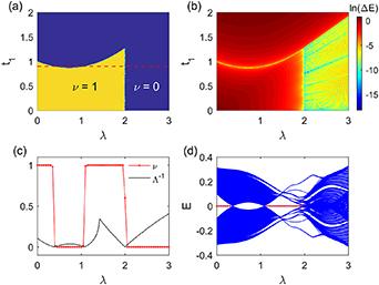
Figure 1. (a) The real-space winding number $\nu$ and (b) the bulk energy gap $\mathrm{ln} \Delta E$ as functions of $\lambda$ and $t_1$. The red dashed line in (a) represents the value of $t_1 = 0.9$. (c) The real-space winding number $\nu$ and the Lyapunov exponent $\Lambda^{-1}$ as a function of $\lambda$ for $t_1 = 0.9$. (d) The middle 200 eigenenergies as a function of $\lambda$ for $t_1 = 0.9$ under OBC. The system size is taken as $L = 2000$ and $\beta = 0.01$. |
To further reveal the reentrant property, we plot the real-space winding number for fixed $t_1 = 0.9$ in figure 1(c). On the other hand, the chiral symmetry is preserved in the disordered SSH chain, so that the localization length at energy $E = 0$ becomes divergent at the topological transition points [48]. We can derive the Lyapunov exponent $\Lambda^{-1}$ (the inverse of the localization length) from equation ($1$) as
$\begin{equation} \begin{aligned} \Lambda^{-1} & = & \left|\lim _{N \rightarrow \infty} \frac{1}{N} \sum_{n = 1}^N\ln\left| \frac{t_2}{t_{1,n}}\right| \right| = \left|\lim _{N \rightarrow \infty} \frac{1}{N} \sum_{n = 1}^N\ln\left| t_{1,n}\right| \right|. \end{aligned}\end{equation}$
The Lyapunov exponent $\Lambda^{-1}$ as a function of $\lambda$ for $t_1 = 0.9$ is depicted by the black line in figure 1(c). Notably, the three divergence points of the localization length coincide with the topological transition points from the real space winding number $\nu$, demonstrating the existence of the multiple reentrant topological transition. In figure 1(d), we plot the middle 200 eigenenergies in the energy spectrum under open boundary condition (OBC) as a function of $\lambda$ for $t_1 = 0.9$. The zero-energy edge modes match well with the results of $\nu$ shown in figure 1(c) owing to the bulk-boundary correspondence.4. Localization properties of the system
To study the localization properties of the eigenstates in the system, we calculate the inverse participation ratio (IPR) and the normalized participation ratio (NPR) for the $n$th eigenstate, which are given by [22]
$\begin{align} \textrm{IPR}_{n}& = \sum_{j = 1}^L|\psi_n^j|^4,\end{align}$
$\begin{align} \textrm{NPR}_{n}& = \left(L\sum_{j = 1}^L|\psi_n^j|^4\right)^{-1},\end{align}$
where $\psi_n^j$ is the amplitude of the $n$th eigenstate at $j$th site. The value of $\textrm{IPR}_{n}\sim 1/L$ and $\textrm{NPR}_n\sim\mathcal {O}(1)$ for an extended eigenstate, while $\textrm{IPR}_n\sim\mathcal{O}(1)$ and $\textrm{NPR}_n\sim 1/L$ for a localized eigenstate. Moreover, one can obtain the mean IPR and the mean NPR defined as $\begin{align} \langle\textrm{IPR}\rangle & = \frac{1}{L}\sum_{n = 1}^L \textrm{IPR}_{n},\end{align}$
$\begin{align} \langle\textrm{NPR}\rangle & = \frac{1}{L}\sum_{n = 1}^L\textrm{NPR}_{n}.\end{align}$
In the large $L$ limit, $\langle\textrm{IPR}\rangle = 0$ ($\neq 0$) and $\langle\textrm{NPR}\rangle\neq0$ ($ = 0$) for the extended (localized) phase. For the intermediate phase, both the $\langle\textrm{IPR}\rangle$ and the $\langle\textrm{NPR}\rangle$ are finite. In order to distinguish the intermediate phase from the extended and the localized phases in the phase diagram, we compute a quantity $\eta$, which is given by [22, 49] $\begin{equation} \eta = \textrm{log}_{10}{\left[{\langle\textrm{IPR}\rangle} \times{\langle\textrm{NPR}\rangle}\right]}.\end{equation}$
If the system is in an extended phase or a localized phase, either $\langle\textrm{IPR}\rangle$ or $\langle\textrm{NPR}\rangle$ scales as $1/L$, and we get $\eta \lt -\textrm{log}_{10}L$. Therefore, $\eta\unicode{x2A7E}-\textrm{log}_{10}L$ corresponds to the intermediate phase. For example, $\eta\unicode{x2A7E}-3.1$ in figure 2 where we have considered $L = 2N = 1220$.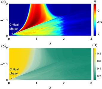
Figure 2. Phase diagram in the $\lambda-t_1$ plane in terms of $\eta$ (a) and $\langle{D}\rangle$ (b) with system size $L = 1220$ and $\beta = 0.01$. In (a), the blue regions represent the extended and localized phases. In (b), the yellow (green) region denotes the extended (localized) phase. |
Moreover, the fractal dimension can be used to accurately identify each eigenstate in different phases, which reads [20, 50]
$\begin{equation}D_n = {-}\mathop{\textrm{lim}}\limits_{L\rightarrow\infty}\frac{\textrm{log}\left(\textrm{IPR}_{n}\right)}{\textrm{log}\left(L\right)}.\end{equation}$
In the large $L$ limit, $D_n$ tends to $1(0)$ for an extended (localized) eigenstate and $0 \lt D_n \lt 1$ for a critical eigenstate. The mean value of the fractal dimension is given by $\begin{equation} \langle{D}\rangle = \frac{1}{L}\sum_{n = 1}^{L} D_{n}.\end{equation}$
When the system is in the extended (localized) phase, the value of $\langle{D}\rangle = 1 (0)$. When $0 \lt \langle{D}\rangle \lt 1$, the system is in the intermediate or critical phase. To further discern the pure critical phase from the intermediate phase, one needs to check if $D_n$ falls between $0$ and $1$ for all the eigenstates.4.1. Phase diagram for small $\beta$
As already mentioned, the potential $V_n(\beta)$ reduces to $V_n = \cos(2\pi \alpha n+\phi)-\cos(\pi \alpha)$ in the $\beta\rightarrow0$ limit, which is the AA modulation with a constant energy shift. Starting from small $\beta$, i.e. $\beta = 0.01$, we plot the phase diagram in the $\lambda-t_1$ plane in terms of $\eta$ and $\langle{D}\rangle$ in figures 2(a) and (b), respectively. The system size is taken as $L = 1220$. When $\beta$ is small, the phase diagram is similar to the case of the AA limit discussed in reference [46]. In figure 2(a), the pure extended and the pure localized phases are denoted by the dark blue regions. The other regions denote the intermediate phase. As $\lambda$ increases, there is a phase transition from the extended phase to the localized phase through the intermediate region. In particular, the system hosts a pure critical phase evidenced by a white arrow in figure 2(a). This pure critical phase can be clearly seen by $\langle{D}\rangle$ in figure 2(b). In figure 2(b), we can also distinguish the extended phase (yellow region) from the localized phase (green region). Therefore, we observe three distinct pure phases in the system, including the extended, localized and critical phases.
For a clear visualization of different pure phases, we calculate the corresponding probability distribution of the single-particle eigenstate $\psi_1^j$ as a function of the site index $j$ in figure 3. The extended state spreads over the whole chain, while the localized state shows a highly localized distribution (see figures 3(a) and (b)). For a critical state, the distribution exhibits a multifractal behavior (see figure 3(c)). We also compute the even–odd and the odd–even level spacings [20, 23, 51], which are defined as
$\begin{align}s^{\mathrm{e-o}}& = E_{2n}-E_{2n-1},\end{align}$
$\begin{align}s^{\mathrm{o-e}}& = E_{2n+1}-E_{2n},\end{align}$
where $E_n$ are the eigenenergies arranged in increasing order. For the extended eigenstate, there is a finite gap between $s^{\mathrm{e-o}}$ and $s^{\mathrm{o-e}}$ (see figure 3(d)). Whereas, this gap vanishes for the localized eigenstate (see figure 3(e)). For the critical eigenstate in figure 3(f), the distributions of $s^{\mathrm{e-o}}$ and $s^{\mathrm{o-e}}$ show noticeable fluctuations.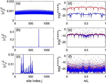
Figure 3. (a)–(c) Density distribution of the single-particle eigenstate $\psi_1^j$ as a function of site index $j$ with system size $L = 1220$. (d)–(f) The even–odd $s^{\mathrm{e-o}}$ (red dots) and odd–even $s^{\mathrm{o-e}}$ (blue dots) level spacings as a function of $n/L$ with system size $L = 13530$. Other parameters are (a), (d) $\lambda = 0.2, t_1 = 1.2$ (extended phase), (b), (e) $\lambda = 1.8, t_1 = 1.5$ (localized phase), and (c), (f) $\lambda = 0.1, t_1 = 0.04$ (critical phase). Here, we set $\beta = 0.01$. |
To explore deeper into the nature of pure phases, we carry out a multifractal and finite-size scaling analysis of the eigenstates. The multifractal behavior of the eigenstates can be identified via the generalized $\mathrm{IPR}$, which is defined as [12, 20, 52],
$\begin{equation} \textrm{IPR}^q_n = \sum_{j = 1}^L|\psi_n^j|^{2q}\sim L^{-\tau_q},\end{equation}$
where $q$ is a real number. $ \textrm{IPR}^q_n$ shows an anomalous scaling with the system size $L$, and $\tau_q$ is a continuous set of exponent. The generalized fractal dimension $D_q$ of the eigenstates can be introduced via $\tau_q = D_q(q-1)$. For an extended and a localized state, $D_q$ is $1$ and $0$, respectively. When $D_q$ is a value between $0$ and $1$, the state is fractal. On the other hand, $0 \lt D_q \lt 1$ with a dependence on $q$ implies the multifractal nature of the eigenstates. In figures 4(a)–(c), we examine the scaling behavior of the generalized $\mathrm{IPR}$ with system size $L$ by considering all eigenstates. For all values of $q$, the exponent $\tau_q$ is linear with $D_q = 1$ for the extended states, and becomes flat for the localized states with $D_q = 0$ (see figures 4(a) and (b)). However, for the critical states shown in figure 4(c), $\tau_q$ changes non-trivially with $q$. In addition to this, the $q$-dependence of the fractal dimension $D_q$ is shown in figure 4(d), which confirms the presence of multifractal states. The critical states observed here display non-trivial multifractal behavior, consistent with general critical states reported previously [53–56]. We confirm that the features of the extended, localized and multifractal states remain stable with increasing system size.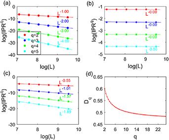
Figure 4. (a)–(c) The generalized IPR versus system size $L$ and different values of $q$ are shown corresponding to (a) $\lambda = 0.2,$ $t_1 = 1.2$, (b) $\lambda = 1.8, t_1 = 1.5$, and (c) $\lambda = 0.1, t_1 = 0.04$. The slope of the curves are characterized by the exponent $\tau_q$. (d) Fractal dimension $D_q$ as a function of $q$ with $ \lambda = 0.1, t_1 = 0.04$ and $L = 13530$. All the plots are shown for $\beta = 0.01$ and all eigenstates in the pure phases. |
In order to have an insight into the intermediate phases shown in figure 2, we plot the fractal dimension $D_n$ of all the eigenstates as a function of $\lambda$ for $t_1 = 0.2$ in figure 5(a) and $t_1 = 1.2$ in figure 5(b), respectively. The regions with red (blue) color for all the eigenstates imply that the system is in the pure extended (localized) phase. For $t_1\,{=}\, 0.2$ in figure 5(a), by increasing $\lambda$, we find that the critical states appear around $n/L\in(0.3,0.7)$. Moreover, the lower and higher eigenstates become localized. Thus, the system hosts an intermediate phase comprising the localized and the critical states. Furthermore, we select $\lambda = 0.5$ and plot the even–odd and odd–even level spacings as a function of the site index in figure 5(c). The distributions of $s^{\mathrm{e-o}}$ and $s^{\mathrm{o-e}}$ show significant fluctuations within the critical region where the states are critical. In the localized region, there is no gap between $s^{\mathrm{e-o}}$ and $s^{\mathrm{o-e}}$. The critical and the localized states in different energy regions are separated by an anomalous ME. For $t_1 = 1.2$ in figure 5(b), in the range $0.6\lesssim\lambda\lesssim2$, the intermediate phase is a mixture of the extended and the localized states which are separated by a traditional ME. Clearly, when $\lambda = 1$ is fixed in figure 5(d), we observe a gap between $s^{\mathrm{e-o}}$ and $s^{\mathrm{o-e}}$ for the middle energy states which are extended.
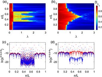
Figure 5. The fractal dimensions $D_n$ of all the eigenstates as a function of $\lambda$ for (a) $t_1 = 0.2$ and (b) $t_1 = 1.2$ with system size $L = 3194$, respectively. The even–odd $s^{\mathrm{e-o}}$ (red dots) and odd–even $s^{\mathrm{o-e}}$ (blue dots) level spacings as a function of $n/L$ for (c) $\lambda = 0.5, t_1 = 0.2$ and (d) $\lambda = 1, t_1 = 1.2$ with system size $L = 13530$. Here, we set $\beta = 0.01$. |
4.2. $\lambda$ induced reentrant localization transition
To study the effect of $\beta$ on the localization properties of the system, we show the phase diagram in the $\lambda-t_1$ plane using $\eta$ for different values of $\beta$ in figure 6. As shown in figure 6(a), $\beta = 1$ has no significant influence on the phase diagram compared to that of figure 2. For $\beta = 1.5$ in figure 6(b), one can see that the intermediate phases emerge in the large $\lambda$ regime. Interestingly, at suitable hopping strengths of $t_1$, the transition from the extended to the localized phase can encounter the intermediate regions multiple times with the increase in $\lambda$, indicating that the system exhibits multiple or reentrant localization transitions [22, 23]. For $\beta = 2.0$ in figure 6(c), the reentrant localization regions move towards the larger $\lambda$ direction. As $\beta$ is further increased (see figures 6(d) and (e)), the reentrant localizations will gradually weaken, and eventually disappear when $\beta$ is fairly large, as shown in figure 6(f).
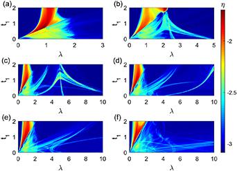
Figure 6. $\eta$ phase diagrams in the $\lambda-t_1$ plane with system size $L = 1220$ for (a) $\beta = 1$, (b) $\beta = 1.5$, (c) $\beta = 2$, (d) $\beta = 2.5$, (e) $\beta = 3$ and (f) $\beta = 5$. |
We also show how the topological phase diagram in the $t_1-\lambda$ plane changes with $\beta$ in figure 7. As $\beta$ increases, the reentrant transition region decreases and the nontopological region increases. Moreover, comparing with figures 7 and 6, it can be seen that the topological phase transition is not tied to the localization transition of the eigenstates.
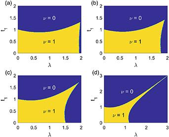
Figure 7. (a)–(d) The real-space winding number as a function of $\lambda$ and $t_1$ for $\beta = 0.5, 1, 2$, and $5$, respectively. The system size is taken as $L = 2000$. |
Next, we analyze in detail the reentrant localization behavior corresponding to $t_1 = 0.7$ and $t_1 = 1.2$ for $\beta = 2.0$ shown in figure 6(c). We first plot the $\langle\textrm{IPR}\rangle$, $\langle\textrm{NPR}\rangle$ and $\eta$ as a function of $\lambda$. For $t_1 = 0.7$ in figure 8(a), there exist four separate intermediate regions located in the shaded regions where both the $\langle\textrm{IPR}\rangle$ and the $\langle\textrm{NPR}\rangle$ are finite. In addition, the increase of $\eta$ in these intermediate regions confirms the presence of the reentrant localization feature. For $t_1 = 1.2$ in figure 8(b), three intermediate phases emerge with the increase in $\lambda$, and the localization transition occurs three times. To reveal the topological properties, we also plot the winding number $\nu$ as a function of $\lambda$ with $\beta = 2.0$ for $t_1 = 0.7$ in figure 8(a) and $t_1 = 1.2$ in figure 8(b), respectively. It is found that the topological phase transition points are not the same as the localization phase transition points.
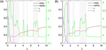
Figure 8. The $\langle\textrm{IPR}\rangle$, $\langle\textrm{NPR}\rangle$, $\eta$, and $\nu$ as a function of $\lambda$ for (a) $t_1 = 0.7$ and (b) $t_1 = 1.2$ with $L = 13530$. Here, $\beta = 2$. The shaded regions mark intermediate phases. |
We further plot the corresponding fractal dimension $D_n$ of all the eigenstates as a function of $\lambda$ in figure 9. In the reentrant localization regions for $t_1 = 0.7$, such as $3.9\lesssim \lambda\lesssim4.3$, $4.9\lesssim \lambda\lesssim5.2$ and $6.6\lesssim \lambda\lesssim7.9$ (see figure 9(a)), some of the already localized states are replaced by the critical states and then localized again as $\lambda$ increases. A similar reentrant feature can also be seen in the second and third intermediate regions for the case of $t_1 = 1.2$ in figure 9(b). Specifically, figure 9(c) shows the values of $D_n$ of all the eigenstates for the intermediate phase when $\lambda = 2.5$ and $t_1 = 0.7$ by increasing the system size. It can be seen that the $D_n$ of the localized eigenstates move towards zero as $L$ increases, while $D_n$ fluctuate around $D_n\simeq0.6$ for the critical eigenstates. When $\lambda = 4.9$ and $t_1 = 1.2$ in figure 9(d), the fractal dimension in different energy regions again confirms that the critical states and the localized states coexist in the intermediate phase.
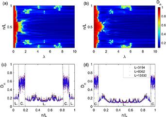
Figure 9. The fractal dimensions $D_n$ of all the eigenstates as a function of $\lambda$ for (a) $t_1 = 0.7$ and (b) $t_1 = 1.2$ with system size $L = 3194$, respectively. The fractal dimension $D_n$ as a function of eigenstate index ratio $n/L$ for (c) $\lambda = 2.5,t_1 = 0.7$ and (d) $\lambda = 4.9,t_1 = 1.2$ with system sizes $L = 3194, 8362$, and $13530$. Here, $\beta = 2$. |
Finally, we show the fractal dimension of all eigenstates as a function of energy and $\beta$ for $\lambda = 3$ and $L = 1220$ in figure 10(a). The lowest set of eigenstates overlaps, delocalizes at $\beta\approx 1.5$, and then localizes again with further increasing $\beta$. In figure 10(b), we plot the $\mathrm{IPR}$ as a function of $\beta$ corresponding to the lowest eigenstate appearing in figure 10(a). The localization-delocalization behavior recurs at different minimums of the $\mathrm{IPR}$ for larger $\beta$. Such reentrant localization of individual states does not occur uniformly, but instead takes place in different parameter regimes depending on the energies of the states [35, 37, 38], which may explain the emergence of multiple reentrant localizations.
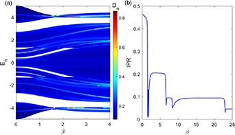


Figure 10. The fractal dimensions $D_n$ of all eigenstates as a function of energy and $\beta$. (b) The IPR of the lowest eigenstate as a function of $\beta$. Here, $L = 1220$ and $\lambda = 3$. |
5. Conclusion
In this paper, we investigate the topological and localization properties in the off-diagonal quasiperiodic SSH model with an IAAF modulation. We obtain the topological phase diagram via the real-space winding number. The behaviors of the bulk gap and the localization length of the zero-energy modes verifies the topological phase boundary. Moreover, the zero-energy edge modes are consistent with the calculation of the real-space winding number. In the AA limit, there exists a topological phase transition from the traditional TI phase to the TAI phase by increasing the quasiperiodic potential strength. Moreover, we find three distinct pure phases, such as the extended, localized and critical phases. Based on the inverse participation ratio, normalized participation ratio, and fractal dimension, we demonstrate the emergent multiple reentrant localization transitions in the system with varying the tunable parameter $\beta$. In the intermediate phase, besides the traditional ME separating the extended and localized states, there is an anomalous ME separating the localized and the critical states. We expect the experimental realization of these findings since the SSH model has been implemented in many artificial systems, such as optical waveguide arrays [57, 58], ultracold atoms [9, 59], and superconducting circuits [60].