Welcome to visit Communications in Theoretical Physics,
Topical Review: Others

Review on memristor application in discrete chaotic system and discrete neuron system

  • Feifei Yang 1 ,
  • Xinlin Song , 2, * ,
  • Ge Zhang 2 ,
  • Huiping Yin 1 ,
  • Jiangxing Chen 3
Expand
  • 1College of Artificial Intelligence and Computer Science, Xi’an University of Science and Technology, Xi’an 710054, China
  • 2College of Science, Xi’an University of Science and Technology, Xi’an 710054, China
  • 3School of Physics, Hangzhou Normal University, Hangzhou 311121, China

*Author to whom any correspondence should be addressed.

Received date: 2025-12-01

  Revised date: 2026-06-09

  Accepted date: 2026-06-10

  Online published: 2026-07-15

Copyright

© 2026 Institute of Theoretical Physics CAS, Chinese Physical Society and IOP Publishing. All rights, including for text and data mining, AI training, and similar technologies, are reserved.
This article is available under the terms of the IOP-Standard License.

Abstract

Continuous memristor nonlinear systems and discrete memristor nonlinear systems are two branches for studying complex dynamical behaviors in nonlinear fields. The nonlinear oscillator modeling based on memristor circuits and the circuit design of memristor nonlinear oscillators have achieved mature research results. However, the modeling of discrete systems based on memristor circuits and the memristor circuit design of map systems are open issues. Therefore, this review systematically elaborates on the precise modeling methods from memristor circuits to discrete dynamical models, and vice versa, to memristor circuits based on the discrete dynamical systems. This review first describes the modeling method from the memristor circuits to the memristor map models. We will construct the equivalent nonlinear map models based on the continuous dynamical oscillators of the memristor oscillation circuits. This process reveals that the connection topology of circuit elements (nonlinear resistors, capacitors, inductors, memristors) directly determines the specific form of the discrete dynamical system. Moreover, this review presents an inverse method from discrete dynamical models to memristor circuits. We demonstrate how to decompose and map the iterative equations of a discrete system into specific memristor circuits. This process reveals that the specific discrete dynamical system can be equivalent to different connection topologies of memristor circuits consisting of nonlinear resistors, capacitors, inductors, and memristors. The two-way framework established in this review profoundly reveals the intrinsic connection between continuous and discrete dynamics in memristor circuits and provides a systematic design methodology for specialized nonlinear hardware systems applicable to fields such as secure communication, true random number generation, and neuromorphic computing.

Cite this article

Feifei Yang , Xinlin Song , Ge Zhang , Huiping Yin , Jiangxing Chen . Review on memristor application in discrete chaotic system and discrete neuron system[J]. Communications in Theoretical Physics, 2026 , 78(9) : 097801 . DOI: 10.1088/1572-9494/ae7b16

1. Introduction

The memristor is the fourth basic circuit element after resistors, capacitors, and inductors. Due to its unique nonlinear memory characteristics and the potential for nano-scale integration, it has sparked a widespread research craze in nonlinear circuits, chaotic systems, brain-inspired computing, and artificial intelligence. The theory of the memristor was first predicted by Professor Chua [1] in 1971. It was not until 2008 when Hewlett-Packard Laboratories achieved a physical prototype in TiO2 material [2] that its dynamic resistance-switching behavior showed similarities to the biomimicry of biological synapses, providing a revolutionary carrier for the next generation of information processing technologies.
The nonlinear characteristic of memristors gives them unique advantages in chaotic circuit design. For example, a memristor chaotic circuit [3] is designed by applying a flux-controlled memristor to replace the nonlinear resistor of the Chua circuit. Bao et al [4] proposed a memristor chaotic circuit based on an active flux-controlled memristor with a smooth, continuous, cubic nonlinearity. Wu and Wang [5] introduced a new memristor for building a simple novel memristor chaotic circuit. Ma et al [6] constructed a memristor chaotic circuit by using a memristor, a memcapacitor, and an inductor. Jin et al [7] developed a locally active memristor from a voltage-controlled memristor for building a simple memristor chaotic circuit. Guo et al [8] built an autonomous memristor chaotic circuit based on a nonlinear current-controlled memristor. These memristor chaotic circuits are obtained by using a memristor and other electrical elements, and they can generate rich nonlinear dynamics. In fact, there are also other chaotic circuits based on memristors. Such as multistability memristive chaotic circuits [9, 10], memristor chaotic circuits with hidden attractors [1113], memristor chaotic circuits with coexisting attractors [1416]. In addition, memristor chaotic systems are obtained by adding one or two memristors to a chaotic system. For instance, multi-stability memristive hyperchaotic systems [17, 18], memristive chaotic systems with hidden attractors [19, 20], memristor chaotic systems with coexisting attractors [2123]. Moreover, memristive chaotic systems are implemented by using the analog circuit hardware [2426] and digital circuit hardware [2729], and they are also used in pseudo-random sequence generators [3032] and image encryption algorithms [3235].
Recently, memristors are widely used in neuroscience. For instance, magnetic flux-controlled memristor neural circuits [36, 37], charge-controlled neural circuit [38], dual memristors neural circuits [39, 40], neural circuits with memristive membrane [4143], neural circuits with memristor ion channel [4446]. These neural circuits are built from memristor-coupled nonlinear circuits. In addition, some memristor neurons are obtained by introducing one or two memristors into a neuron model presented by differential equations, for instance, HR memristive neuron [47], FHN memristive neuron [48], and memristor-coupled neuron systems [49, 50]. Furthermore, memristor neuron models are also implemented by using the analog circuit hardware [51, 52] and digital circuit hardware [53], and they are also used in pseudo-random sequence generators [54] and image encryption algorithms [55]. Moreover, there are many memristor neural networks [5658]. For more research on memristors in neurons and networks, readers can refer to the reviews [59, 60]. In addition, reservoir computing based on the nonlinear dynamical properties of memristors in the temporal information processing and physical computing are researched in [61, 62].
Discrete systems have lower computational complexity and more diverse dynamic behaviors compared to continuous systems. Chaos is particularly typical in discrete maps. Analyzing the dynamics of discrete chaotic systems not only reveals the universal path of nonlinear systems moving from order to disorder, but also provides a rigorous mathematical framework for understanding the unpredictability of complex systems. Additionally, constructing neuron models in discrete time can significantly improve computational efficiency while retaining the key discharge characteristics of biological neurons. This discretization processing breaks through the step size limitations and hardware implementation bottlenecks of traditional continuous differential equations, making it possible to simulate large-scale neural networks. The discrete memristor is not a new type of device that has different physical properties from continuous-time memristors. Instead, it refers to a method or model for implementing the function and behavior of a memristor in a discrete-time system. The core idea is to use discrete-time iterative operations to simulate the continuous and history-dependent resistance state changes of a memristor. A discrete memristor has significant advantages in enhancing system performance, increasing dynamic complexity, improving computational efficiency, and achieving neuro-like functions. Therefore, discrete memristor chaotic systems and discrete memristor neurons are widely researched in recent years. For example, 2-dimensional discrete memristor chaotic system [63], 3-dimensional discrete memristor chaotic system [64], high-dimensional discrete memristor chaotic system [65], hyperchaotic discrete memristive systems [6668]. In addition, discrete memristive chaotic systems are implemented based on digital circuit hardware [6971], and they are used in image encryption algorithms [7274]. Furthermore, there are many discrete memristor neurons proposed, such as the 2-dimensional memristive Chialvo neuron map [75], the diffusively delay-coupled memristive Chialvo neuron map [76], and the electrochemically coupled memristive Rulkov neuron map [77]. Moreover, there are many other memristive neuron maps [7880] and memristive map neuron networks [8183].
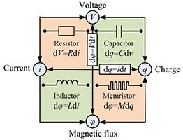
Metabolic energy maintains the vitality of biological neurons, while physical energy, named neuron energy, clarifies the dynamical mechanism for mode transition in electrical activities, and synchronization stability between neurons, formation of defects, and heterogeneity in the neural networks. Most of the neurons can simulate the electrical activities in many equivalent neural circuits, which are composed of capacitors, inductors, memristors, resistors, and nonlinear resistors. The field energy in the neural circuit is saved in the capacitive, inductive, and memristive elements. By applying a scale transformation on the physical variables in the nonlinear equations and field energy for the neural circuit, a dimensionless neuron model and Hamilton energy will be obtained for further nonlinear analysis. The energy function of the memristive map is defined in [84, 85]. Therefore, this review primarily introduces the discrete memristive models developed from the memristor-coupled nonlinear circuits and the verification of the chaotic maps expressed based on the mathematical iterative equations by applying the memristor-coupled nonlinear circuit. As is well known, a nonlinear circuit can be built by using a nonlinear electrical element and other electrical components. Memristor is a nonlinear electrical element, and it reveals the interrelationship between magnetic flux (φ) and charge (q). Figure 1 plotted the relationship diagram of the voltage (V), current (i), magnetic flux (φ), and charge (q).
Figure 1. The relationship among resistor (R), inductor (L), capacitor (C), and memristor (M).
From figure 1, the variables (V, i, φ, q) have six mathematical equations, and they are described by applying electrical elements (R, L, C, M), Faraday’s Law of electromagnetic induction (dφ = Vdt), and the relationship between electric charge and current (dq = idt). A memristor is a nonlinear electronic component with the physical dimension of resistance. Memristors are classified into magnetic flux-controlled memristors (MFCM, the resistance value depends on the magnetic flux) and charge-controlled memristors (CCM, the resistance value depends on the charge).
The relationship between the current and voltage in MFCM is expressed by
$\begin{align}{i_M} = M\left(\varphi \right){v_M};\frac{{{\text{d}}\varphi }}{{{\text{d}}t}} = f\left(\varphi ,{v_M}\right),\end{align}$
where M(φ) denotes the memductance, and it can be described by applying a function with the magnetic flux. (iM, vM) are the output current and input voltage across the memristor, respectively. According to [59], the field energy of the MFCM can be calculated by using the field energy of an inductor with a suitable inductance LM, and then the field energy function of an MFCM can be obtained by
$\begin{align}{W_M} = \frac{1}{2}{L_M}i_M^2 = \frac{1}{2}\varphi {i_M}.\end{align}$
Similarly, the volt–ampere characteristic of a CCM is estimated by
$\begin{align}{v_W} = W\left(q\right){i_W};\frac{{{\text{d}}q}}{{{\text{d}}t}} = g\left(q,{i_W}\right),\end{align}$
where W(q) means the mean-resistance. (iW, vW) denotes the input current and output voltage in the CCM, respectively. According to [59], the field energy of the CCM is estimated by using the field energy of an equivalent capacitor. Therefore, the field energy function of a CCM can be described as follows
$\begin{align}{H_W} = \frac{1}{2}{C_W}v_W^2 = \frac{1}{2}q{v_W}.\end{align}$

2. Modeling of discrete chaotic systems based on memristor circuits
The discrete memristive chaotic system is a kind of chaotic system based on discrete memristors, and its research mainly focuses on how to utilize the nonlinear characteristics of memristors to enhance the chaotic characteristics of the system. This type of system can achieve more complex chaotic behaviors by introducing the discrete memristor model, such as expanding chaotic regions, increasing complexity, generating hyperchaotic sequences, and so on. The construction of discrete memristor chaotic systems is widely researched. However, it is very interesting research on the memristive chaotic maps built by the memristor-coupled nonlinear circuit.
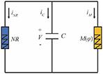
In [86], a two-dimensional MFCM chaotic map is constructed from an MFCM-coupled nonlinear circuit. Figure 2 is a memristor-coupled nonlinear circuit without an inductor.
Figure 2. An MFCM-coupled nonlinear circuit without an inductor. NR is a nonlinear resistor; C denotes a capacitor, and M(φ) means an MFCM.
In figure 2, the equation of the circuit state variable is described as follows
$\begin{equation}\left\{ \begin{aligned} C\frac{{{\text{d}}V}}{{{\text{d}}t}} &= \frac{r}{\rho }\left(V - \frac{{{V^2}}}{{{V_0}}}\right) - \varphi V,\\ \frac{{{\text{d}}\varphi }}{{{\text{d}}t}} &= \alpha \varphi + \beta V.\\ \end{aligned} \right.\end{equation}$
The dimensionless equation in equation (5) is described by
$\begin{equation}\left\{ \begin{aligned} \frac{{{\text{d}}x}}{{{\text{d}}t}} &= - cwxr + \left(x - {x^2}\right),\\ \frac{{{\text{d}}w}}{{{\text{d}}t}} &= \beta x + aw.\\ \end{aligned} \right.\end{equation}$
The parameters and variables in equation (6) can be calculated as follows
$\begin{equation}\left\{ \begin{aligned} x &= \frac{V}{{{V_0}}},w = \frac{\varphi }{{\rho C{V_0}}},\tau = \frac{t}{{\rho C}},\\ c &= {\rho ^2}C{V_0},a = \alpha \rho C.\\ \end{aligned} \right.\end{equation}$
The field energy function of the electrical elements in figure 2 is estimated by
$\begin{equation}\left\{ \begin{aligned}W&=\frac{1}{2}C{V^2} + \frac{1}{2}\varphi {i_M},\\ H&=\frac{W}{{CV_0^2}}=\frac{1}{2}{x^2}+\frac{1}{2}c{w^2}x.\\\end{aligned}\right.\end{equation}$
Furthermore, a memristor chaotic map is built based on equation (6), and the result is described as follows
$\begin{equation}\left\{ \begin{aligned}{y_{n + 1}} &= \lambda \left({y_n} - y_n^2\right) - \gamma {y_n}{z_n},\\ {z_{n + 1}} &= \delta {y_n} + \mu {z_n}.\\\end{aligned}\right.\end{equation}$
Similarly, parameters and variables in equation (9) are calculated by
$\begin{equation}\left\{\begin{aligned}{y_n}&=\frac{{r\Delta\tau}}{{1+r\Delta\tau}}{x_n},{z_n}=\frac{{r\Delta \tau }}{{1 + r\Delta \tau }}{w_n},\\ \lambda &=1+r\Delta\tau,\delta=a\Delta\tau+1,\gamma=c\Delta\tau,\mu=b\Delta\tau.\\\end{aligned}\right.\end{equation}$
In addition, the energy function of the memristive chaotic map is calculated
$\begin{align}{H_n} = \frac{1}{2}{y_n} + \frac{1}{2}\gamma z_n^2{y_n}.\end{align}$
In [86], a two-dimensional CCM chaotic map is obtained by applying a CCM-coupled nonlinear circuit without a capacitor. The circuit diagram of a CCM nonlinear circuit consists of a CCM, a nonlinear resistor, and a constant voltage source, as plotted in figure 3.
Figure 3. A CCM-coupled nonlinear circuit without a capacitor. NR is a nonlinear resistor; L denotes an inductor, and M(q) means a CCM.
The equations of a CCM-coupled nonlinear circuit without a capacitor in figure 3 are described as follows
$\begin{equation}\left\{\begin{aligned}L\frac{{{\text{d}}{i_L}}}{{{\text{d}}t}}&=r\rho \left({i_L} - \frac{{\rho i_L^2}}{{{V_0}}}\right) - \left(\alpha + 3\beta {q^2}\right){i_L} - E,\\ \frac{{{\text{d}}q}}{{{\text{d}}t}} &= aq + b{i_L}.\\\end{aligned}\right.\end{equation}$
The dimensionless equations for the memristor-coupled nonlinear circuit are expressed by variables as follows
$\begin{equation}\left\{ \begin{aligned}\frac{{{\text{d}}y}}{{{\text{d}}t}}&=r\left(y - {y^2}\right) - d - \left(\alpha ^{\prime} + \beta ^\prime{u^2}\right)y,\\ \frac{{{\text{d}}u}}{{{\text{d}}t}} &= by + a^{\prime} u.\\\end{aligned}\right.\end{equation}$
The parameters and variables in equation (13) can be calculated as follows
$\begin{equation}\left\{ \begin{aligned}y &=\frac{{\rho {i_L}}}{{{V_0}}},u=\frac{{{\rho ^2}q}}{{L{V_0}}},\tau =\frac{{\rho t}}{L},\\ \alpha ^{\prime} &= \frac{\alpha }{\rho },\beta ^{\prime} = \frac{{3\beta {L^2}V_0^2}}{{{\rho ^5}}},a^{\prime} = \frac{{aL}}{\rho },d = \frac{E}{{{V_0}}}.\\ \end{aligned}\right.\end{equation}$
The field energy for the memristor-coupled nonlinear circuit in figure 3 and its dimensionless energy function are calculated by
$\begin{align}\left\{ \begin{gathered} {W_2} = \frac{1}{2}Li_L^2 + \frac{1}{2}{C_M}V_M^2 = \frac{1}{2}Li_L^2 + \frac{1}{2}q{V_M},\\ {H_2} = \frac{{{W_2}}}{{V_0^2\left(L/{\rho ^2}\right)}} = \frac{1}{2}{y^2} + \frac{1}{2}\left(\alpha ^{\prime} u + \beta ^\prime{u^3}\right)y.\\ \end{gathered} \right.\end{align}$
Furthermore, the parameters and variables in equation (13) are defined as follows
$\begin{align}\left\{ {\begin{array}{*{20}{l}} {{w_n} = \frac{{r\Delta \tau }}{{1 + r\Delta \tau }}{y_n},{v_n} = \frac{{r\Delta \tau }}{{1 + r\Delta \tau }}{u_n},\chi = 1 + r\Delta \tau ,\xi = {\alpha ^{\prime} }\Delta \tau ,} \\ {\varepsilon = \frac{{{\beta ^{\prime} }{{\left(1 + r\Delta \tau \right)}^2}}}{{{r^2}\Delta \tau }},\kappa = a\Delta \tau + 1,\eta = b\Delta \tau ,{d^{\prime} } = d\Delta \tau .} \end{array}} \right.\end{align}$
A two-dimensional CCM map is described by
$\begin{equation}\left\{ \begin{aligned}{w_{n + 1}} &= \chi \left({w_n} - w_n^2\right) - \left(\zeta + \varepsilon v_n^2\right){w_n} - d^{\prime} ,\\ {v_{n + 1}}&=\kappa{w_n}+\eta {v_n}.\\\end{aligned}\right.\end{equation}$
The energy function for the two-dimensional discrete memristor system in equation (17) can be obtained as follows
$\begin{align}{H^{\prime}_n} = \frac{1}{2}{w_n} + \frac{1}{2}\left(\xi + \varepsilon v_n^2\right){w_n}{v_n}.\end{align}$
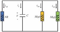
Furthermore, in [87], a dual memristor discrete system is developed from a two-memristor-coupled nonlinear circuit without an inductor. Figure 4 is a dual memristor-coupled nonlinear circuit without an inductor.
Figure 4. A dual memristor-coupled nonlinear circuit without an inductor. NR is a nonlinear resistor, C denotes a capacitor, M(φ) means an MFCM, and M(q) is a CCM.
The circuit equations of the dual memristor-coupled nonlinear circuit in figure 4 are obtained as follows
$\begin{equation}\left\{\begin{aligned}C\frac{{{\text{d}}V}}{{{\text{d}}t}}&=\frac{r}{\rho }\left(V - \frac{{{V^2}}}{{{V_0}}}\right) - \sin qV - \varphi V,\\ \frac{{{\text{d}}\varphi }}{{{\text{d}}t}} &= bV + a\varphi ,\\ \frac{{{\text{d}}q}}{{{\text{d}}t}} &= \sin qV + dq.\\\end{aligned}\right.\end{equation}$
To obtain the dimensionless equations of equation (19), the parameters and variables are redefined in equation (20).
$\begin{align}\left\{ \begin{gathered} x = \frac{V}{{{V_0}}},w = \frac{\varphi }{{\rho C{V_0}}},u = \frac{q}{{C{V_0}}},\tau = \frac{t}{{\rho C}},\\ a = {\rho ^2}C{V_0},k = C{V_0},c = a\rho C,d^{\prime} = dC\rho ,\alpha = \rho .\\ \end{gathered} \right.\end{align}$
As a result, equation (19) can be reexpressed by
$\begin{equation}\left\{\begin{aligned}\frac{{{\text{d}}x}}{{{\text{d}}t}}&=- awxr + \left(x - {x^2}\right) - \alpha \sin \left(ku\right)x,\\ \frac{{{\text{d}}w}}{{{\text{d}}t}} &= bx + cw,\\ \frac{{{\text{d}}u}}{{{\text{d}}t}} &= \alpha \sin \left(ku\right)x + d^{\prime} u.\\\end{aligned}\right.\end{equation}$
The field energy in figure 4 and its dimensionless energy are calculated as follows
$\begin{align}\left\{ \begin{gathered} W = \frac{1}{2}C{V^2} + \frac{1}{2}\varphi {i_{M1}} + \frac{1}{2}qV,\\ H = \frac{W}{{CV_0^2}} = \frac{1}{2}{x^2} + \frac{1}{2}a{w^2}x + \frac{1}{2}ux.\\ \end{gathered} \right.\end{align}$
To build a dual memristive chaotic map, the parameters and variables in equation (21) are reupdated by
$\begin{equation}\left\{\begin{aligned}{y_n}&=\frac{{r\Delta \tau }}{{1 + r\Delta \tau }}{x_n},{z_n} = \frac{{r\Delta \tau }}{{1 + r\Delta \tau }}{w_n},\\{v_n} &= \frac{{r\Delta \tau }}{{1 + r\Delta \tau }}{u_n},\lambda = 1 + r\Delta \tau ,\\ b &= \frac{{1 + r\Delta \tau }}{r},\beta = \alpha \Delta \tau ,\delta = k\frac{{1 + r\Delta \tau }}{{r\Delta \tau }},\\a &= c\Delta \tau + 1;d = d^{\prime}\Delta \tau + 1,c = b\Delta \tau .\end{aligned}\right.\end{equation}$
A dual memristor discrete system can be expressed as follows
$\begin{equation}\left\{\begin{aligned}{y_{n + 1}}&=\lambda \left({y_n} - y_n^2\right) - b{y_n}{z_n} - \beta \sin \left(\delta {v_n}\right){y_n},\\ {z_{n + 1}} &= a{y_n} + c{z_n};\\ {v_{n + 1}} &= d{v_n} + \beta \sin \left(\delta {v_n}\right){y_n}.\\\end{aligned}\right.\end{equation}$
The energy function of the discrete memristor system in equation (24) is described by
$\begin{align}{H_n} = \frac{1}{2}{y_n} + \frac{1}{2}bz_n^2{y_n} + \frac{1}{2}{v_n}{y_n}.\end{align}$
In [88], a controllable memristive chaotic map is generated from a simple memristor circuit. The memristive circuit diagram is shown in figure 5.
Figure 5. A controllable memristor circuit without an inductor. NR is a nonlinear resistor, C denotes a capacitor, M(φ) means an MFCM, and is denotes an external current.
The circuit equation presented in figure 5 can be obtained as follows
$\begin{align}\left\{ {\begin{array}{*{20}{l}} {C\frac{{{\text{d}}V}}{{{\text{d}}t}} = {i_s} + \frac{r}{\rho }\left( {V - \frac{{{V^2}}}{{{V_0}}}} \right) - \varphi V,} \\ {\frac{{{\text{d}}\varphi }}{{{\text{d}}t}} = \alpha \varphi + \beta V.} \end{array}} \right.\end{align}$
The variables in equation (26) are updated by
$\begin{align}x = \frac{V}{{{V_0}}},w = \frac{\varphi }{{\rho C{V_0}}},\tau = \frac{t}{{\rho C}}.\end{align}$
Therefore, the equations in equation (26) are described as follows
$\begin{equation}\left\{ \begin{aligned}\frac{{{\text{d}}x}}{{{\text{d}}\tau }} &= {u_s} - cwx + r\left(x - {x^2}\right),\\ \kern-24pt \frac{{{\text{d}}w}}{{{\text{d}}\tau }} &= \beta x + aw,\end{aligned}\right.\end{equation}$
where parameters in equation (28) are defined by
$\begin{align}c = {\rho ^2}C{V_0},a = \alpha \rho C,{u_s} = \frac{{\rho {i_s}}}{{{V_0}}}.\end{align}$
For the memristive circuit in figure 5, its physical field energy is calculated as follows
$\begin{align}W = \frac{1}{2}C{V^2} + \frac{1}{2}{L_M}i_M^2 = \frac{1}{2}C{V^2} + \frac{1}{2}\varphi {i_M}.\end{align}$
The energy corresponding to equation (30) can be updated by
$\begin{align}H = \frac{W}{{CV_0^2}} = \frac{1}{2}{x^2} + \frac{1}{2}c{w^2}x.\end{align}$
The variables in equation (28) are further defined by
$\begin{align}{y_n} = \frac{{r\Delta \tau }}{{1 + r\Delta \tau }}{x_n},{z_n} = \frac{{r\Delta \tau }}{{1 + r\Delta \tau }}{w_n}.\end{align}$
And then a memristive map is given as follows
$\begin{align}\left\{ {\begin{array}{*{20}{l}} {{y_{n + 1}} = {i_s} + \lambda \left( {{y_n} - y_n^2} \right) - \gamma {y_n}{z_n},} \\ {{z_{n + 1}} = \delta {y_n} + \mu {z_n},} \end{array}{\text{ }}} \right.\end{align}$
where the parameters in equation (33) can be calculated by
$\begin{align}\mu = b\Delta \tau ,\lambda = 1 + r\Delta \tau ,\delta = a\Delta \tau + 1,\gamma = c\Delta \tau ,{i_s} = \frac{{r{{\left(\Delta \tau \right)}^2}}}{{1 + r\Delta \tau }}\!.\end{align}$
Moreover, an energy function of the chaotic map is defined as follows
$\begin{align}{H_n} = \frac{1}{2}{y_n} + \frac{1}{2}\gamma z_n^2{y_n}.\end{align}$
In summary, modeling discrete chaotic systems based on memristor circuits serves as an important bridge connecting cutting-edge electronic devices with nonlinear dynamics theory. The core idea lies in utilizing the unique memory characteristics and nonlinear resistance-switching behavior of memristors to construct discrete chaotic systems that are physically feasible and functionally rich. By ingeniously combining memristors with simple linear circuit elements (such as capacitors and inductors), more complex second-order or higher-order discrete systems can be constructed. For instance, in a circuit composed of electronic components like memristors and capacitors, a two-dimensional nonlinear mapping can be established. This circuit achieves an accurate transformation from continuous physical dynamics to discrete mathematical iterations.

3. Modeling of discrete neurons based on memristor circuits
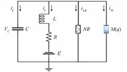
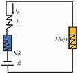
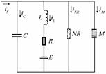
The discrete memristor neuron model can be established by combining the nonlinear characteristics of memristors with the dynamic characteristics of discrete-time systems. The discrete memristor neuron model provides new perspectives and methods for the modeling, analysis, and application of neural networks, and it has extensive research value and engineering potential. Therefore, the modeling of the memristive neuron map is becoming a research hotspot. In [89], a CCM neuron map is developed from a CCM-coupled nonlinear circuit. Figure 6 plots a CCM-coupled nonlinear circuit.
Figure 6. CCM-coupled nonlinear circuit. NR is a nonlinear resistor, C denotes a capacitor, L means an inductor, R is a linear resistor, E denotes a voltage source, and M(q) is a CCM.
The output equations in figure 6 are described by
$\begin{equation}\left\{\begin{aligned}C\frac{{{\text{d}}{V_C}}}{{{\text{d}}t}}&=-{i_L}+\frac{r}{\rho }\left({V_C} - \frac{{V_C^2}}{{{V_0}}}\right) - {\frac{{{V_C}}}{{{k_M}\left(\alpha + 3\beta {q^2}\right)}}_M},\\ L\frac{{{\text{d}}{i_L}}}{{{\text{d}}t}} &= {V_C} + E - {i_L}R,\\ \frac{{{\text{d}}q}}{{{\text{d}}t}} &= {\frac{{{V_C}}}{{{k_M}\left(\alpha + 3\beta {q^2}\right)}}_M} + \xi q.\\\end{aligned}\right.\end{equation}$
The field energy in figure 6 is calculated by
$\begin{align}W = \frac{1}{2}CV_C^2 + \frac{1}{2}L{i_L}^2 + \frac{1}{2}{C_M}V_M^2 = \frac{1}{2}CV_C^2 + \frac{1}{2}L{i_L}^2 + \frac{1}{2}q{V_M}.\end{align}$
Furthermore, the variables and parameters in equations (36) and (37) can be reupdated as follows
$\begin{align}\left\{ \begin{gathered} x = \frac{{{V_C}}}{{{V_0}}},y = \frac{{\rho {i_L}}}{{{V_0}}},z = \frac{q}{{C{V_0}}},\tau = \frac{t}{{\rho C}},a = \frac{{{k_M}\alpha }}{\rho },\\ b = \frac{{3{k_M}{C^2}V_0^2\beta }}{\rho },c = \frac{{\rho {C^2}}}{L},d = \frac{E}{{{V_0}}},e = \frac{R}{\rho },f = \xi \rho C.\\ \end{gathered} \right.\end{align}$
As a result, a CCM neuron is expressed by
$\begin{equation}\left\{ \begin{aligned}\frac{{{\text{d}}x}}{{{\text{d}}\tau }} &= - y + rx\left(1 - x\right) - \frac{x}{{a + b{z^2}}},\\ \frac{{{\text{d}}y}}{{{\text{d}}\tau }} &= c\left(x - ey + d\right),\\ \frac{{{\text{d}}z}}{{{\text{d}}\tau }} &= fz + \frac{x}{{a + b{z^2}}}.\\ \end{aligned} \right.\end{equation}$
The dimensionless energy function of a CCM neuron can be presented as follows
$\begin{align}H = \frac{W}{{CV_0^2}} = \frac{1}{2}{x^2} + \frac{1}{{2c}}{y^2} + \frac{1}{2}xz.\end{align}$
To obtain a CCM neuron map, the discrete variables of the neuron presented in equation (39) can be expressed as
$\begin{equation}\left\{\begin{aligned}{x_n}&=\frac{{r\Delta \tau }}{{1 + r\Delta \tau }}{x^{^{\prime}}_n},{y_n} = \frac{{r\Delta \tau }}{{1 + r\Delta \tau }}{y^{^{\prime}}_n},{z_n} = \frac{{r\Delta \tau }}{{1 + r\Delta \tau }}{z^{^{\prime}}_n},\\\eta &= 1 + r\Delta \tau ,\delta ^{\prime} = \Delta \tau ,a^{\prime} = \frac{a}{{\Delta \tau }},\\ b^{\prime} &= \frac{{{{\left(1 + r\Delta \tau \right)}^2}}}{{{r^2}\Delta {\tau ^3}}}b,c^{\prime} = c\Delta \tau ,d^{\prime} = \frac{{r\Delta \tau }}{{1 + r\Delta \tau }}d,\\e^{\prime} &= \frac{1}{{c\Delta \tau }} - e,f^{\prime} = f\Delta \tau + 1.\\ \end{aligned}\right.\end{equation}$
Furthermore, a CCM map neuron is described as follows
$\begin{equation}\left\{ \begin{aligned}{x_{n + 1}} &= \eta {x_n}\left(1 - {x_n}\right) - \delta ^\prime{y_n} - \frac{{{x_n}}}{{a^{\prime} + b^{^{\prime}}z_n^2}},\\ {y_{n + 1}} &= c^{\prime}\left({x_n} + d^{\prime} + e^\prime{y_n}\right),\\ {z_{n + 1}} &= \frac{{{x_n}}}{{a^{\prime} + b^{^{\prime}}z_n^2}} + f^\prime{z_n}.\\ \end{aligned} \right.\end{equation}$
In addition, the energy function of the CCM map neuron presented in equation (42) can be expressed by
$\begin{align}{H_n} = \frac{{{W_n}}}{{CV_0^2}} = {H^{\prime}_n} + {H^{^{\prime\prime}}_n} + {H^{^{\prime\prime}\!^{\prime}}_n} = \frac{1}{2}x_n^2 + \frac{1}{{2c^{\prime}}}y_n^2 + \frac{1}{2}{x_n}{z_n}.\end{align}$
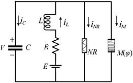
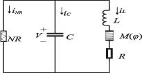
In [90], an MFCM map neuron is built based on an MFCM-coupled nonlinear circuit. The corresponding nonlinear circuit is displayed in figure 7.
Figure 7. A MFCM-coupled nonlinear circuit. NR is a nonlinear resistor, C denotes a capacitor, L means an inductor, R is a linear resistor, E denotes a voltage source, and M(φ) is an MFCM.
The equations of an MFCM-coupled nonlinear circuit are described by
$\begin{equation}\left\{\begin{aligned}C\frac{{{\text{d}}{V_C}}}{{{\text{d}}t}}&={i_L} + \frac{r}{\rho }\left({V_C} - \frac{{V_C^2}}{{{V_0}}}\right) - \left({\alpha _1} + 3{\beta _1}{\phi ^2}\right){V_C},\\ L\frac{{{\text{d}}{i_L}}}{{{\text{d}}t}} &= E - V - {i_L}R,\\ \frac{{{\text{d}}\phi }}{{{\text{d}}t}}&=A\phi + BV.\\ \end{aligned}\right.\end{equation}$
The variables and parameters in equation (44) are redefined in equation (45).
$\begin{align}\left\{ \begin{gathered} x = \frac{V}{{{V_0}}},y = \frac{{{i_L}\rho }}{{{V_0}}},\tau = \frac{t}{{\rho C}},\varphi ^{\prime} = \frac{\phi }{{\rho C{V_0}}},\alpha ^{\prime} = {\alpha _1}\rho ,\\ \beta ^{\prime} = {\beta _1}{\rho ^3}{C^2}{V_0}^2,A^{\prime} = A\rho C,a = \frac{E}{{{V_0}}},b = \frac{{{\rho ^2}C}}{L},c = \frac{R}{\rho }.\\ \end{gathered} \right.{\kern 1pt} \end{align}$
A dimensionless neuron is updated as follows
$\begin{equation}\left\{ \begin{aligned} \frac{{{\text{d}}x}}{{{\text{d}}\tau }} &= r\left(x - {x^2}\right) + y - x\left(\alpha ^{\prime} + 3\beta ^\prime{{\varphi ^{\prime}}^2}\right),\\ \frac{{{\text{d}}y}}{{{\text{d}}\tau }} &= b\left( - cy + a - x\right),\\ \frac{{{\text{d}}\varphi ^{\prime}}}{{{\text{d}}\tau }} &= Bx + A^{\prime}\varphi ^{\prime}.\\ \end{aligned} \right.{\kern 1pt}\end{equation}$
Field energy of an MFCM neuron and its dimensionless energy function are calculated as follows
$\begin{align}\left\{ \begin{gathered} W = \frac{1}{2}C{V^2} + \frac{1}{2}Li_L^2 + \frac{1}{2}{L_M}i_M^2 = \frac{1}{2}C{V^2} + \frac{1}{2}Li_L^2 + \frac{1}{2}\phi {i_M},\\ H = \frac{{{W_1}}}{{CV_{_0}^2}} = \frac{1}{2}{x^2} + \frac{1}{{2b}}{y^2} + \frac{1}{2}\left(\alpha ^{\prime}\varphi ^{\prime} + 3\beta ^\prime{{\varphi ^{\prime}}^3}\right)x.\\ \end{gathered} \right.\end{align}$
The discrete variables and parameters in equation (46) are redefined in equation (48) for obtaining a map neuron.
$\begin{equation}\left\{\begin{aligned}{z_n}&=\frac{{r\Delta\tau}}{{1 + r\Delta \tau }}{x_n},{w_n} = \frac{{r\Delta \tau }}{{1 + r\Delta \tau }}{y_n},{\varphi _n} = \frac{{r\Delta \tau }}{{1 + r\Delta \tau }}{\varphi ^{^{\prime}}_n},\\ \alpha &= \alpha ^{\prime}\Delta \tau ,\lambda = 1 + r\Delta \tau , \beta = \frac{{\beta ^{\prime}{{\left(1 + r\Delta \tau \right)}^2}}}{{\Delta \tau {r^2}}},\\k &= \Delta \tau ,d = \frac{{r\Delta {\tau ^2}}}{{1 + r\Delta \tau }}a,f = c\Delta \tau - \frac{1}{b},\\ \eta &= A^{\prime}\Delta \tau + 1,\mu = B\Delta \tau .\\ \end{aligned}\right.\end{equation}$
As a result, an MFCM map neuron can be described as follows
$\begin{equation}\left\{\begin{aligned}{z_{n + 1}}&=\lambda \left({z_n} - z_n^2\right) - {z_n}\left(\alpha + 3\beta {\varphi _n}^2\right) + k{w_n},\\ {w_{n + 1}} &= b\left(d - k{z_n} - f{w_n}\right),\\ {\varphi _{n + 1}} &= \eta {\varphi _n} + \mu {z_n}.\\ \end{aligned}\right.\end{equation}$
In addition, the energy function of the discrete memristive neuron map is calculated by
$\begin{align}{H_n} = \frac{1}{2}{z_n}^2 + \frac{1}{{2b}}{w_n}^2 + \frac{1}{2}\left(\alpha {\varphi _n} + 3\beta {\varphi _n}^3\right){z_n}.\end{align}$
In [91], a dual memristor discrete neuron is obtained by applying a dual memristor-coupled nonlinear circuit. Figure 8 displayed a dual memristor-coupled nonlinear circuit.
Figure 8. A dual memristor-coupled nonlinear circuit. NR is a nonlinear resistor, C denotes a capacitor, L means an inductor, R is a linear resistor, M(φ) denotes an MFCM, and M(q) is a CCM.
The equivalent dynamical equations in figure 8 are presented as
$\begin{equation}\left\{ \begin{aligned} C\frac{{{\text{d}}V}}{{{\text{d}}t}} &= - {i_L} + \frac{r}{r}\left( {V - \frac{{{V^2}}}{{{V_0}}}} \right) - \varphi V,\\ L\frac{{{\text{d}}{i_L}}}{{{\text{d}}t}} &= V - q{i_M} - R{i_L},\\ \frac{{{\text{d}}q}}{{{\text{d}}t}} &= aq + b{i_M},\\ \frac{{{\text{d}}\varphi }}{{{\text{d}}t}} &= a\varphi + b{V_\varphi }.\\ \end{aligned} \right.\end{equation}$
Furthermore, the variables in equation (52) are replaced by
$\begin{align}x = \frac{V}{{{V_0}}},y = \frac{{\rho {i_L}}}{{{V_0}}},z = \frac{q}{{C{V_0}}},w = \frac{\varphi }{{\rho C{V_0}}},\tau = \frac{t}{{\rho C}}.\end{align}$
As a result, the dynamical equations in equation (51) are expressed as follows
$\begin{equation}\left\{ \begin{aligned} \frac{{{\text{d}}x}}{{{\text{d}}t}} &= - y + r\left( {x - {x^2}} \right) - cwx,\\ \frac{{{\text{d}}y}}{{{\text{d}}t}} &= d\left( {x - ezy - gy} \right)\!,\\ \frac{{{\text{d}}z}}{{{\text{d}}t}} &= a^{\prime} z + by,\\ \frac{{{\text{d}}w}}{{{\text{d}}t}} &= a^{\prime} w + bx,\\ \end{aligned} \right.\end{equation}$
where parameters in equation (53) are obtained by
$\begin{align}c = {\rho ^2}C{V_0},d = \frac{{{\rho ^2}C}}{L},e = \frac{{C{V_0}}}{\rho },g = \frac{R}{\rho },\alpha ^{\prime} = \rho \alpha C,a^{\prime} = a\rho C.\end{align}$
The corresponding field energy of the dual memristor-coupled nonlinear circuit is calculated as follows
$\begin{align}W &= {W_C} + {W_L} + {W_M} + {W_\varphi }\nonumber\\ & = \frac{1}{2}C{V^2} + \frac{1}{2}Li_L^2 + \frac{1}{2}{q^2}{i_L} + \frac{1}{2}{\varphi ^2}V.\end{align}$
Furthermore, the dimensionless energy in equation (55) is obtained by
$\begin{align}H & = \frac{W}{{CV_0^2}} = {H_C} + {H_L} + {H_M} + {H_\varphi } \nonumber\\ & = \frac{1}{2}{x^2} + \frac{1}{{2d}}{y^2} + \frac{1}{2}e{z^2}y + \frac{1}{2}c{w^2}x.\end{align}$
The variables in equation (53) are redefined as follows
$\begin{align}{x^{\prime}_n} &= \frac{{r\Delta \tau }}{{1 + r\Delta \tau }}{x_n},{y^{\prime}_n} = \frac{{r\Delta \tau }}{{1 + r\Delta \tau }}{y_n},{z^{\prime}_n} = \frac{{r\Delta \tau }}{{1 + r\Delta \tau }}{z_n},\nonumber\\ {w^{\prime}_n} & = \frac{{r\Delta \tau }}{{1 + r\Delta \tau }}{w_n}.\end{align}$
As a result, a dual memristor map neuron can be presented as follows
$\begin{equation}\left\{ \begin{aligned} {x^{^{\prime}}_{n + 1}} &= - {\lambda _1}{y^{^{\prime}}_n} + {r_1}\left( {{x^{^{\prime}}_n} - {x^{^{\prime}}_n}^2} \right) - {c_1}{w^{^{\prime}}_n}{x^{^{\prime}}_n},\\ {y^{^{\prime}}_{n + 1}} &= {d_1}\left( {{x^{^{\prime}}_n} - {e_1}{z^{^{\prime}}_n}{y^{^{\prime}}_n} - {g_1}{y^{^{\prime}}_n}} \right)\!,\\ {z^{^{\prime}}_{n + 1}} &= {\alpha _1}{z^{^{\prime}}_n} + {\beta _1}{y^{^{\prime}}_n},\\ {w^{^{\prime}}_{n + 1}} &= {a_1}{w^{^{\prime}}_n} + {b_1}{x^{^{\prime}}_n}.\\ \end{aligned} \right.\end{equation}$
The parameters in equation (58) can be obtained as follows
$\begin{equation}\begin{aligned}\left\{ {\begin{array}{*{20}{l}}{{\lambda_1}= \Delta \tau ,{r_1} = 1 + r\Delta \tau ,{c_1} = c\frac{{1 + r\Delta \tau }}{r},{d_1} = d\Delta \tau ,}\\{{e_1} = e\frac{{1 + r\Delta \tau }}{{r\Delta \tau }}, {g_1} = g - \frac{1}{{d\Delta \tau }},{\alpha _1} = 1 + \alpha ^{\prime}\Delta \tau ,} \\{{\beta_1}=\beta \Delta \tau ,{a_1} = 1 + a^{\prime}\Delta \tau \!,{b_1} = b\Delta \tau.}\end{array}}\right.\end{aligned}\end{equation}$
Similarly, the energy function of the dual memristor map neuron in equation (58) can be calculated by
$\begin{align}{H_n} = \frac{1}{2}x^{^{\prime} 2}_n + \frac{1}{{2{d_1}}}y^{^{\prime} 2}_n + \frac{1}{2}{e_1}z^{^{\prime} 2}_n y^{^{\prime}_n} + \frac{1}{2}{c_1}w^{^{\prime} 2}_n x^{^{\prime}_n}.\end{align}$
Yang et al [92] proposed a memristor circuit without an inductor, and the circuit is shown in figure 9.
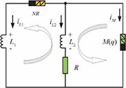
Figure 9. A memristive circuit without a capacitor. NR is a nonlinear resistor, L1 and L2 are two inductors, R is a linear resistor, and M(q) is a CCM.
Based on Kirchhoff’s laws, the circuit equations in figure 9 are given as follows
$\begin{equation}\left\{ \begin{aligned} {L_1}\frac{{{\text{d}}{i_{L1}}}}{{{\text{d}}t}} &= r\rho \left({i_{L1}} - \frac{{\rho i_{L1}^2}}{{{V_0}}}\right) - q\left({i_{L1}} + {i_{L2}}\right)\!,\\ {L_2}\frac{{{\text{d}}{i_{L2}}}}{{{\text{d}}t}} &= - q\left({i_{L1}} + {i_{L2}}\right) - R{i_{L2}},\\ \frac{{{\text{d}}q}}{{{\text{d}}t}} &= \alpha q + \beta \left({i_{L1}} + {i_{L2}}\right)\!.\\ \end{aligned} \right.\end{equation}$
The variables and parameters in equation (61) are defined by
$\begin{align}\left\{ \begin{gathered} x = \frac{{\rho {i_{L1}}}}{{{V_0}}},y = \frac{{\rho {i_{L2}}}}{{{V_0}}},z = \frac{{{\rho ^2}q}}{{{L_1}{V_0}}},\tau = \frac{{\rho t}}{{{L_1}}},\\ c = \frac{{{L_1}}}{{{L_2}}},a = \frac{{{L_1}{V_0}}}{{{\rho ^3}}},b = \frac{R}{\rho },\alpha ^{\prime} = \frac{{{\alpha _1}{L_1}}}{\rho }.\\ \end{gathered} \right.\end{align}$
According to equations (61) and (62), an oscillator is described by
$\begin{equation}\left\{ \begin{aligned} \frac{{{\text{d}}x}}{{{\text{d}}\tau }} &= r\left(x - {x^2}\right) - az\left(x + y\right)\!,\\ \frac{{{\text{d}}x}}{{{\text{d}}\tau }} &= c\left[ - az\left(x + y\right) - by\right]\!,\\ \frac{{{\text{d}}z}}{{{\text{d}}\tau }} &= \alpha ^{\prime} z + \beta \left(x + y\right)\!.\\ \end{aligned} \right.\end{equation}$
The physical field energy for figure 9 and its dimensionless energy function H can be calculated by
$\begin{equation}\left\{ \begin{aligned} W &= {W_{L1}} + {W_{L2}} + {W_M} = \frac{1}{2}{L_1}i_1^{^2} + \frac{1}{2}{L_2}i_2^{^2} + \frac{1}{2}q{V_M},\\ H &= \frac{{{W_{L1}} + {W_{L2}} + {W_M}}}{{V_0^2{L_1}/{\rho ^2}}} = {H_{L1}} + {H_{L2}} + {H_M}\\ &= \frac{1}{2}{x^2} + \frac{1}{{2c}}{y^2} + \frac{1}{2}a{z^2}\left(x + y\right).\\ \end{aligned} \right.\end{equation}$
Furthermore, a group of new discrete variables and parameters in equation (63) is defined as follows
$\begin{equation}\left\{ \begin{aligned} {x_n} &= \frac{{r\Delta \tau }}{{1 + r\Delta \tau }}{u_n},{y_n} = \frac{{r\Delta \tau }}{{1 + r\Delta \tau }}{v_n},{z_n} = \frac{{r\Delta \tau }}{{1 + r\Delta \tau }}{w_n},\\ \delta &= \frac{{a\left(1 + r\Delta \tau \right)}}{r},\lambda = 1 + r\Delta \tau ,\gamma = \frac{{bc\Delta \tau - 1}}{c},\\ \kappa &= 1 + \alpha ^{\prime}\Delta \tau ,\eta = \beta \Delta \tau . \end{aligned} \right.\end{equation}$
A memristive map of the memristive oscillator in equation (63) can be described by
$\begin{equation}\left\{ \begin{aligned} {u_{n + 1}} &= \lambda \left({u_n} - u_n^2\right) - \delta {w_n}\left({u_n} + {v_n}\right)\!,\\ {v_{n + 1}} &= c\left[ - \delta {w_n}\left({u_n} + {v_n}\right) - \gamma {v_n}\right]\!,\\ {w_{n + 1}} &= \kappa {w_n} + \eta \left({u_n} + {v_n}\right)\!.\\ \end{aligned} \right.\end{equation}$
Furthermore, a similar energy function is calculated by
$\begin{align}{H_n} = \frac{1}{2}u_n^2 + \frac{1}{{2c}}v_n^2 + \frac{1}{2}\delta w_n^2\left({u_n} + {v_n}\right)\!.\end{align}$
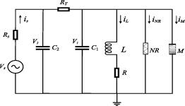
Guo et al [93] proposed a memristive neural circuit with a thermosensitive membrane, and its circuit is plotted in figure 10.
The current for the nonlinear resistor and memristor in figure 10 is estimated as follows
$\begin{equation}\left\{ \begin{aligned} {i_{NR}} &= - \frac{r}{\rho }\left({V_1} - \frac{{{V_1}^2}}{{{V_0}}}\right)\!\!,\\ {V_M} &= M\left(q\right){i_M} = \frac{{\csc \left(q\right)}}{{{\lambda _1}}} \cdot {i_M} = {V_1}.\\ \end{aligned} \right.\end{equation}$
Figure 10. A memristive neural circuit with a thermosensitive membrane. NR is a nonlinear resistor, C1 and C2 denote two capacitors, L means an inductor, Rs and R are two linear resistors, RT denotes a thermistor, Vs is a voltage source and M is a CCM.
The field energy in figure 10 is described by
$\begin{align}W = \frac{1}{2}{C_1}{V_1}^2 + \frac{1}{2}{C_2}{V_2}^2 + \frac{1}{2}L{i_L}^2 + \frac{1}{2}q{V_M}.\end{align}$
The correlation between physical variables in figure 10 is obtained as follows
$\begin{equation}\left\{ \begin{aligned} {C_2}\frac{{{\text{d}}{V_2}}}{{{\text{d}}t}} &= {i_s} - \frac{{{V_2} - {V_1}}}{{{R_T}}},\\ {C_1}\frac{{{\text{d}}{V_1}}}{{{\text{d}}t}} &= \frac{{{V_2} - {V_1}}}{{{R_T}}} - {i_L} - {i_{NR}} - {i_M},\\ L\frac{{{\text{d}}{i_L}}}{{{\text{d}}t}} &= {V_1} - {i_L}R,\\ \frac{{{\text{d}}q}}{{{\text{d}}t}} &= {\lambda _2}q + {i_M}.\\ \end{aligned} \right.\end{equation}$
The new variables and parameters are defined as follows
$\begin{equation}\left\{ \begin{aligned} x &= \frac{{{V_2}}}{{{V_0}}},y = \frac{{{V_1}}}{{{V_0}}},z = \frac{{\rho {i_L}}}{{{V_0}}},\tau = \frac{t}{{\rho {C_2}}},{u_s} = \frac{{\rho {V_s}}}{{{R_s}{V_0}}},\\a &= \frac{{\rho R{C_2}}}{L}, b = \frac{\rho }{{{R_s}}} + \frac{\rho }{{{R_T}}}, c = \frac{\rho }{{{R_T}}},d = \frac{{{\rho ^2}{C_2}}}{L},\\ \alpha &= \frac{{{C_2}}}{{{C_1}}},u = \frac{q}{{{C_2}{V_0}}},f = \rho {\lambda _1},k = {C_2}{V_0}, g = {\lambda _2}\rho {C_2}.\\ \end{aligned} \right.\end{equation}$
Consequently, the dynamic equation of a memristive neuron can be described by
$\begin{equation}\left\{ \begin{aligned} \frac{{{\text{d}}x}}{{{\text{d}}\tau }} &= {u_s} - bx + cy,\\ \frac{{{\text{d}}y}}{{{\text{d}}\tau }} &= \alpha \left[ {c\left( {x - y} \right) - z + r\left( {y - {y^2}} \right) - f\sin \left(ku\right)y} \right],\\ \frac{{{\text{d}}z}}{{{\text{d}}\tau }} &= dy - az,\\ \frac{{{\text{d}}u}}{{{\text{d}}\tau }} &= gu + f\sin \left(ku\right)y.\\ \end{aligned} \right.\end{equation}$
The dimensionless Hamilton energy function H corresponding to the field energy W in equation (69) is presented as follows
$\begin{align}H = \frac{W}{{{C_2}V_0^2}} = \frac{1}{2}{x^2} + \frac{1}{{2\alpha }}{y^2} + \frac{1}{{2d}}{z^2} + \frac{1}{2}uy.\end{align}$
The new parameters and discrete variables are defined by
$\begin{equation}\left\{ \begin{aligned} {x_n}^{\prime} &= \frac{{r\Delta \tau }}{{1 + r\Delta \tau }}{x_n},{y_n}^{\prime} = \frac{{r\Delta \tau }}{{1 + r\Delta \tau }}{y_n},{z_n}^{\prime} = \frac{{r\Delta \tau }}{{1 + r\Delta \tau }}{z_n},\\ {u_n}^{\prime} &= \frac{{r\Delta \tau }}{{1 + r\Delta \tau }}{u_n}, {u_s}^{\prime} = \frac{{r\Delta {\tau ^2}}}{{1 + r\Delta \tau }}{u_s},{b_1} = b\Delta \tau - 1,\\{c_1} &= c\Delta \tau ,{\alpha _1} = \alpha \Delta \tau , {d_1} = 1 + \frac{1}{{\alpha r\Delta \tau }}, {g_1} = a\Delta \tau - 1,\\{l_1} &= k\frac{{1 + r\Delta \tau }}{{r\Delta \tau }},{l_2} = d\Delta \tau ,{l_3} = g\Delta \tau + 1, {l_4} = f\Delta \tau .\\ \end{aligned} \right.\end{equation}$
A map neuron of equation (72) can be described as follows
$\begin{equation}\left\{ \begin{aligned} {x^{^{\prime}}_{n + 1}} &= {u^{^{\prime}}_s} - {b_1}{x^{^{\prime}}_n} + {c_1}{y^{^{\prime}}_n},\\ {y^{^{\prime}}_{n + 1}} &= {\alpha _1}\left[c\left({x_n}^{\prime} - {y_n}^{\prime} \right) - {z^{^{\prime}}_n} + r\left({d_1}{y^{^{\prime}}_n} - {y^{^{\prime}}_n}^2\right)\right. \\ &\left.- f\sin \left({l_1}{u^{^{\prime}}_n}\right){y^{^{\prime}}_n}\right],\\ {z^{^{\prime}}_{n + 1}} &= {l_2}{y^{^{\prime}}_n} - {g_1}{z^{^{\prime}}_n},\\ {u^{^{\prime}}_{n + 1}} &= {l_3}{u^{^{\prime}}_n} + {l_4}\sin \left({l_1}{u^{^{\prime}}_n}\right){y^{^{\prime}}_n}.\\ \end{aligned} \right.\end{equation}$
A similar energy function for a map neuron can be presented by
$\begin{align}{H_n} = \frac{1}{2}x^{^{\prime} 2}_n + \frac{1}{{2{\alpha _1}}}y^{^{\prime} 2}_n + \frac{1}{{2{l_2}}}z^{^{\prime} 2}_n + \frac{1}{2}{u^{^{\prime}}_n}{y^{^{\prime}}_n}.\end{align}$
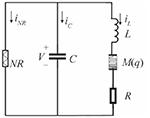
Chen et al [94] designed a neural circuit with a hybrid ion channel, and a neural circuit is plotted in figure 11.
Figure 11. Schematic diagram for a neural circuit with a hybrid ion channel. NR is a nonlinear resistor, C denotes a capacitor, L means an inductor, R is a linear resistor, and M(q) is a CCM.
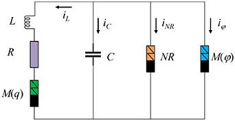
The relationship of the variables in figure 11 is described as follows
$\begin{equation}\left\{ \begin{aligned} C\frac{{\text{d}V}}{{\text{d}t}} &= \frac{r}{\rho }\left(V - \frac{{{V^2}}}{{{V_0}}}\right) - {i_L},\\ L\frac{{\text{d}{i_L}}}{{\text{d}t}} &= V - \left(\alpha + 3\beta {q^2}\right){i_L} - {i_L}R,\\ \frac{{\text{d}q}}{{\text{d}t}} &= k{i_L} + \varepsilon q.\\ \end{aligned} \right.\end{equation}$
The field energy in figure 11 is estimated by
$\begin{align}W = {W_1} + {W_2} + {W_3} = \frac{1}{2}C{V^2}\; + \frac{1}{2}Li_L^2 + \frac{1}{2}q{V_M}.\end{align}$
To minimize the influence of physical dimensions, the dimensionless variables and parameters are adopted as follows
$\begin{align}\left\{ \begin{gathered} x = \frac{V}{{{V_0}}},y = \frac{{\rho {i_L}}}{{{V_0}}},\tau = \frac{t}{{\rho C}},c = \frac{{{\rho ^2}C}}{L},u = \frac{q}{{C{V_0}}},\\ \alpha = \frac{R}{\rho },f = \varepsilon \rho C,a = \frac{\alpha }{\rho },b = \frac{{3\beta {C^2}V_0^2}}{\rho }.\\ \end{gathered} \right.\end{align}$
Consequently, the memristive neural circuit defined in equation (77) gives rise to an oscillator whose dynamics are captured by the following dimensionless model in equation (80),
$\begin{equation}\left\{ \begin{aligned} \frac{{\text{d}x}}{{{\text{d}}\tau }} &= r\left(x - {x^2}\right) - y,\\ \frac{{\text{d}y}}{{\text{d}\tau }} &= c\left[x - \alpha y - \left(a + b{u^2}\right)y\right],\\ \frac{{\text{d}u}}{{\text{d}\tau }} &= ky + fu.\\ \end{aligned} \right.\end{equation}$
Thus, the field energy in equation (78) is expressed in dimensionless form as the Hamilton energy function in equation (81),
$\begin{align}\left\{ \begin{gathered} {H_C} = \frac{1}{2}{x^2};{H_L} = \frac{1}{{2c}}{y^2};{H_M} = \frac{1}{2}\left(au + b{u^3}\right)y,\\ H = \frac{W}{{C{V_0}^2}} = \frac{1}{2}{x^2} + \frac{1}{{2c}}{y^2} + \frac{1}{2}\left(au + b{u^3}\right)y.\\ \end{gathered} \right.\end{align}$
The parameters and variables in equation (80) are updated as follows
$\begin{equation}\left\{ \begin{aligned} {Z_n} &= \frac{{r\vartriangle \tau }}{{1 + r\vartriangle \tau }}{x_n},\;{W_n} = \frac{{r\vartriangle \tau }}{{1 + r\vartriangle \tau }}{y_n},\;{V_n} = \frac{{r\vartriangle \tau }}{{1 + r\vartriangle \tau }}{u_n},\\ \lambda &= 1 + r\vartriangle \tau ,\gamma = \vartriangle \tau ; d = \alpha \vartriangle \tau - \frac{1}{c},\\ a^{\prime} &= a\vartriangle \tau ,\;b^{\prime} = b\frac{{{{\left(1 + r\vartriangle \tau \right)}^2}}}{{{r^2}\vartriangle \tau }}, \beta = f\vartriangle \tau + 1,\;\delta = k\vartriangle \tau .\\ \end{aligned} \right.\end{equation}$
And then, a memristive map is given as
$\begin{equation}\left\{ \begin{aligned} {Z_{n + 1}} &= \lambda \left({Z_n} - {Z_n}^2\right) - \gamma {W_n},\\ {W_{n + 1}} &= c\left[\gamma {Z_n} - d{W_n} - \left(a^{\prime} + b^{\prime} V_n^2\right){W_n}\right],\\ {V_{n + 1}} &= \delta {W_n} + \beta {V_n}.\\ \end{aligned} \right.\end{equation}$
An energy function of the discrete form in equation (83) can be obtained as follows
$\begin{align}\left\{ \begin{aligned} & {H_{Cn}} = \frac{1}{2}Z_n^2,{H_{Ln}} = \frac{1}{{2c}}W_n^2,{H_{Mn}} = \frac{1}{2}\left(a^\prime{V_n} + b^\prime{V_n}^3\right){W_n},\\ & {H_n} = \frac{1}{2}Z_n^2 + \frac{1}{{2c}}W_n^2 + \frac{1}{2}\left(a^\prime{V_n} + b^\prime{V_n}^3\right){W_n}{\text{.}} \end{aligned} \right.\end{align}$
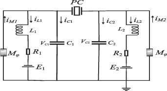
Li et al [95] considered a scenario in which the intracellular and extracellular media exhibit distinct electromagnetic field gradients and energy levels on either side of the cell membrane. To emulate the resulting variability in capacitive properties and the influence of membrane material characteristics, they incorporated two capacitors connected via a piezoelectric component. Additionally, two memristors were introduced into the neural circuit illustrated in figure 12 to account for specific field-induced effects.
Figure 12. A neural circuit with a piezoelectric membrane. C1 and C2 denote two capacitors, L1 and L2 are two inductors, R1 and R2 are two linear resistors, PC denotes a piezoelectric ceramic, E1 and E2 are two voltage sources, and M(φ) denotes two MFCM.
The correlation of physical variables in figure 12 is described as follows
$\begin{equation}\left\{ \begin{aligned} {C_1}\frac{{\text{d}{V_{C1}}}}{{\text{d}t}} &= {i_{M1}} - {i_{L1}} - {i_s},\quad\\ {C_2}\frac{{\text{d}{V_{C2}}}}{{\text{d}t}} &= {i_{M2}} - {i_{L2}} + {i_s},\\ {L_1}\frac{{\text{d}{i_{L1}}}}{{\text{d}t}} &= {V_{C1}} + {E_1} - {i_{L1}}{R_1},\quad\\ {L_2}\frac{{\text{d}{i_{L2}}}}{{\text{d}t}} &= {V_{C2}} + {E_2} - {i_{L2}}{R_2},\\ \frac{{\text{d}{\phi _1}}}{{\text{d}t}} &= {a_1}{\phi _1} + b{V_{C1}},\quad \\ \frac{{\text{d}{\phi _2}}}{{\text{d}t}} &= {\eta _1}{\phi _2} + \mu {V_{C2}}.\\ \end{aligned} \right.\end{equation}$
The current in equation (85) is respectively approached by
$\begin{equation}\left\{ \begin{aligned} {i_s} &= \left({V_{C1}} - {V_{C2}}\right)/{R_S},\\ {i_{M1}} &= {M_1}\left({\phi _1}\right){V_{C1}} = \left({\alpha _1} + 3{\beta _1}{\phi _1}^2\right){V_{C1}},\\ {i_{M2}} &= {M_2}\left({\phi _2}\right){V_{C2}} = {\phi _2}{V_{C2}}.\\ \end{aligned} \right.\end{equation}$
The dimensionless variables and parameters are defined in equation (87).
$\begin{equation}\left\{\begin{aligned}x^{\prime}&=\frac{{{V_{C1}}}}{{{E_1}}},y^{\prime} = \frac{{{V_{C2}}}}{{{E_1}}},z^{\prime} = \frac{{{i_{L1}}{R_1}}}{{{E_1}}},w^{\prime} = \frac{{{i_{L2}}{R_1}}}{{{E_1}}},\\ {\varphi _1} &= \frac{{{\phi _1}}}{{{R_1}{C_1}{E_1}}}\!\!, {\varphi _2} = \frac{{{\phi _2}}}{{{R_1}{C_1}{E_1}}}\!,\\ \tau &= \frac{t}{{{R_1}{C_1}}},\alpha ^{\prime} = {\alpha _1}{R_1},\beta ^{\prime} = {\beta _1}{C_1}^2{E_1}^2{R_1}^3,\\ \alpha {^{^{\prime\prime}}} &= {R_1}^2{E_1}{C_1}, {\delta _1} = \frac{{{R_1}}}{{{R_S}}},{\delta _2} = \frac{{{C_1}}}{{{C_2}}},\\ {\delta _3} &= \frac{{{R_1}^2{C_1}}}{{{L_1}}},{\delta _4} = \frac{{{R_1}^2{C_1}}}{{{L_2}}},{\delta _5} = \frac{{{E_2}}}{{{E_1}}},\\ {\delta _6} &= \frac{{{R_2}}}{{{R_1}}},a = {a_1}{R_1}{C_1}, \eta = {\eta _1}{R_1}{C_1}.\\ \end{aligned} \right.\end{equation}$
Therefore, a neuron with piezoelectric membrane can be described by
$\begin{equation}\left\{\begin{aligned}\frac{{{\text{d}}x^{\prime}}}{{{\text{d}}\tau }} &= \left(\alpha ^{\prime} + 3\beta ^\prime{\varphi _1}^2\right)x^{\prime} - z^{\prime} - {\delta _1}\left(x^{\prime} - y^{\prime}\right),\\ \frac{{{\text{d}}y^{\prime}}}{{{\text{d}}\tau }} &= {\delta _2}\left[\alpha ^{^{\prime\prime}}{y^{\prime}}{\varphi _2} - w^{\prime} + {\delta _1}\left(x^{\prime} - y^{\prime}\right)\right],\\ \frac{{{\text{d}}z^{\prime}}}{{{\text{d}}\tau }} &= {\delta _3}\left(x^{\prime} + 1 - z^{\prime}\right),\\ \frac{{{\text{d}}w^{\prime}}}{{{\text{d}}\tau }} &= {\delta _4}\left(y^{\prime} + {\delta _5} - {\delta _6}w^{\prime}\right),\\ \frac{{{\text{d}}{\varphi _1}}}{{{\text{d}}\tau }} &= a{\varphi _1} + bx^{\prime},\\ \frac{{{\text{d}}{\varphi _2}}}{{{\text{d}}\tau}} &= \eta {\varphi _2} + \mu y^{\prime}.\\ \end{aligned}\right.\end{equation}$
The physical energy in figure 12 and its equivalent dimensionless energy form are presented as follows
$\begin{equation}\left\{\begin{aligned}W&=\frac{1}{2}{C_1}{V_{C1}}^2 + \frac{1}{2}{C_2}{V_{C2}}^2 + \frac{1}{2}{L_1}i_{L1}^2 + \frac{1}{2}{L_2}i_{L2}^2 \\&+ \frac{1}{2}{L_{M1}}i_{M1}^2 + \frac{1}{2}{L_{M2}}i_{M2}^2\\ &= \frac{1}{2}{C_1}{V_{C1}}^2 + \frac{1}{2}{C_2}{V_{C2}}^2 + \frac{1}{2}{L_1}i_{L1}^2 + \frac{1}{2}{L_2}i_{L2}^2 \\&+ \frac{1}{2}{\phi _1}{i_{M1}} + \frac{1}{2}{\phi _2}{i_{M2}},\\ H &= \frac{W}{{{C_1}E_1^2}} = \frac{1}{2}{{x^{\prime}}^2} + \frac{1}{{2{\delta _2}}}{{y^{\prime}}^2} + \frac{1}{{2{\delta _3}}}{{z^{\prime}}^2} \\ &+ \frac{1}{{2{\delta _4}}}{{w^{\prime}}^2} + \frac{1}{2}\left(\alpha ^\prime{\varphi _1} + 3\beta ^{\prime}\varphi _1^3\right)x^{\prime} + \frac{1}{2}\alpha ^{^{\prime\prime}}\varphi _2^2y^{\prime}.\\ \end{aligned}\right.\end{equation}$
The parameters and variables in equation (88) are given as follows
$\begin{equation}\left\{ \begin{aligned}{x_n} &= \frac{{r\Delta \tau }}{{1 + r\Delta \tau }}{x^{^{\prime}}_n},{y_n} = \frac{{r\Delta \tau }}{{1 + r\Delta \tau }}{y^{^{\prime}}_n},\\{z_n} &= \frac{{r\Delta \tau }}{{1 + r\Delta \tau }}{z^{^{\prime}}_n}, {w_n} = \frac{{r\Delta \tau }}{{1 + r\Delta \tau }}{w^{^{\prime}}_n}, \\ {u_n} &= \frac{{r\Delta \tau }}{{1 + r\Delta \tau }}{\varphi _1}_n,{v_n} = \frac{{r\Delta \tau }}{{1 + r\Delta \tau }}{\varphi _2}_n,\\{\alpha _1} &= \frac{{1 + r\Delta \tau }}{r}\alpha ^{^{\prime\prime}}, \beta = \frac{{\beta ^{\prime}{{(1 + r\Delta \tau )}^2}}}{{\Delta \tau {r^2}}}, \\ \alpha &= \alpha ^{\prime}\Delta \tau ,{\lambda _1} = \Delta \tau ,{\lambda _2} = {\delta _1}\Delta \tau ,\\{\lambda _3} &= 1 - \frac{1}{{{\lambda _2}}}, {\lambda _4} = \frac{1}{{{\delta _2}{\lambda _2}}} - 1,{\lambda _5} = {\delta _3}\Delta \tau , \\ {\lambda _6} &= \frac{{r\Delta \tau }}{{1 + r\Delta \tau }},{\lambda _7} = 1 - \frac{1}{{{\lambda _5}}},{\lambda _8} = {\delta _4}\Delta \tau ,\\{\lambda _9} &= \frac{{r\Delta \tau }}{{1 + r\Delta \tau }}{\delta _5}, {\lambda _{10}} = {\delta _6} - \frac{1}{{{\lambda _8}}}, \\ {a_2} &= 1 + a\Delta \tau ,{b_1} = b\Delta \tau ,{\eta _2} = 1 + \eta \Delta \tau ,\\{\mu _1} &= \mu \Delta \tau , {{u^{^{\prime\prime}}}_{{\text{ext}}}} = \frac{{r\Delta \tau }}{{1 + r\Delta \tau }}{u^{^{\prime}}_{{\text{ext}}}}. \\ \end{aligned}\right.\end{equation}$
And then a map neuron can be described as follows
$\begin{equation}\left\{ \begin{aligned}{x_{n + 1}} &= \left(\alpha + 3\beta {u_n}^2\right){x_n} - {\lambda _1}{z_n} - {\lambda _2}\left({\lambda _3}{x_n} - {y_n}\right),\\ {y_{n + 1}} &= {\delta _2}\left[{\alpha _1}{y_n}{v_n} - {\lambda _1}{w_n} + {\lambda _2}\left({x_n} - {\lambda _4}{y_n}\right)\right],\\ {z_{n + 1}} &= {\lambda _5}\left({x_n} + {\lambda _6} - {\lambda _7}{z_n}\right),\\ {w_{n + 1}} &= {\lambda _8}\left({y_n} + {\lambda _9} - {\lambda _{10}}{w_n}\right),\\ {u_{n + 1}} &= {a_2}{u_n} + {b_1}{x_n},\\ {v_{n + 1}} &= {\eta _2}{v_n} + {\mu _1}{y_n}.\\ \end{aligned}\right.{\kern 1pt}\end{equation}$
Similarly, a energy function can be estimated as
$\begin{align}{H_n} & = \frac{1}{2}{x_n}^2 + \frac{1}{{2{\delta _2}}}{y_n}^2 + \frac{1}{{2{\lambda _5}}}{z_n}^2 \nonumber\\ &\quad + \frac{1}{{2{\lambda _8}}}{w_n}^2 + \frac{1}{2}\left(\alpha {u_n} + 3\beta {u_n}^3\right){x_n} + \frac{1}{2}{\alpha _1}v_n^2{y_n}.\end{align}$
Wang et al [96] designed a memristive neural circuit in figure 13. This neural circuit is consisted of a capacitor, an inductor, a nonlinear resistor, a linear resistor and a MFCM.
Figure 13. A memristor-coupled neural circuit. NR is a nonlinear resistor, C denotes a capacitor, L means an inductor, R is a linear resistors and M(φ) is a MFCM.
The relations of the physical variables are approached as follows
$\begin{equation}\left\{\begin{aligned}C\frac{{{\text{d}}V}}{{{\text{d}}t}} &= \frac{r}{\rho }\left(V - \frac{{{V^2}}}{{{V_0}}}\right) - {i_L},\\ L\frac{{{\text{d}}{i_L}}}{{{\text{d}}t}} &= V - {i_L}R - {V_M},\\ \frac{{{\text{d}}\varphi }}{{{\text{d}}t}} &= A\varphi + B{V_M}.\\ \end{aligned}\right.\end{equation}$
The parameters and variables in equation (93) are updated by
$\begin{align}\left\{ \begin{gathered} x = \frac{V}{{{V_0}}},y = \frac{{\rho {i_L}}}{{{V_0}}},\tau = \frac{t}{{C\rho }},z = \frac{\varphi }{{{V_0}C\rho }},\xi = \frac{1}{{\mu L{V_0}}},\\ \alpha = \frac{{C{\rho ^2}}}{L},\beta = \frac{{C\rho R}}{L},A^{\prime} = AC\rho ,B^{\prime} = \frac{B}{{\mu C{\rho ^2}{V_0}}}.\\ \end{gathered} \right.\end{align}$
Therefore, the circuit equations in equation (93) can be replaced as follows
$\begin{align}\left\{ \begin{gathered} \frac{{{\text{d}}x}}{{{\text{d}}\tau }} = r\left(x - {x^2}\right) - y,\\ \frac{{{\text{d}}y}}{{{\text{d}}\tau }} = \alpha x - \beta y - \xi \frac{y}{z},\\ \frac{{{\text{d}}z}}{{{\text{d}}\tau }} = A^{\prime} z + B^{\prime}\frac{y}{z}.\\ \end{gathered} \right.\end{align}$
From figure 13, the field energy and its dimensionless form are given by
$\begin{equation}\left\{\begin{aligned}W&=\frac{1}{2}C{V^2}\; + \frac{1}{2}Li_L^2 + \frac{1}{2}\varphi {i_M} \\&= CV_0^2\left(\frac{1}{2}{x^2} + \frac{1}{{2\alpha }}{y^2} + \frac{1}{2}yz\right),\\ H &= \frac{W}{{CV_0^2}} = \frac{1}{2}{x^2} + \frac{1}{{2\alpha }}{y^2} + \frac{1}{2}yz.\\ \end{aligned}\right.\end{equation}$
The variables (x, y, z) and parameters are linear transformed as follows
$\begin{equation}\left\{\begin{aligned}{u_n}&=\frac{{r\Delta \tau }}{{1 + r\Delta \tau }}{x_n},{v_n} = \frac{{r\Delta \tau }}{{1 + r\Delta \tau }}{y_n},\\{w_n} &= \frac{{r\Delta \tau }}{{1 + r\Delta \tau }}{z_n}, \lambda = 1 + r\Delta \tau,\\ a &= 1 - \beta \Delta \tau ,b = \frac{{\xi r{{\left(\Delta \tau \right)}^2}}}{{1 + r\Delta \tau }},c = 1 + A^{\prime}\Delta \tau,\\d &= \Delta \tau , e = \alpha \Delta \tau ,f = \frac{{B^{\prime} r{{\left(\Delta \tau \right)}^2}}}{{1 + r\Delta \tau }}.\\ \end{aligned}\right.\end{equation}$
Therefore, a new map neuron can be presented by
$\begin{equation}\left\{ \begin{aligned}{u_{n + 1}} &= \lambda \left({u_n} - {u_n}^2\right) - d{v_n},\\ {v_{n + 1}} &= e{u_n} + a{v_n} - b{v_n}/{w_n},\\ {w_{n + 1}} &= c{w_n} + f{v_n}/{w_n}.\\ \end{aligned}\right.\end{equation}$
The energy function for map neuron in equation (98) can be approached as follows
$\begin{equation}\left\{ \begin{aligned}H_n^C &= \frac{1}{2}{u_n}^2,H_n^L = \frac{1}{{2e}}{v_n}^2,H_n^M = \frac{1}{2}{v_n}{w_n},\\ {H_n} &= H_n^C + H_n^L + H_n^M = \frac{1}{2}{u_n}^2 + \frac{1}{{2e}}{v_n}^2 + \frac{1}{2}{v_n}{w_n}.\\ \end{aligned}\right.\end{equation}$
Lei et al [97] proposed a memristor-coupled neural circuit, and its circuit diagram is shown in figure 14.
Figure 14. Memristor-coupled neural circuit. NR is a nonlinear resistor, C denotes a capacitor, L means an inductor, E denotes a voltage source, R is a linear resistors and M(q) is a CCM.
In figure 14, the circuit equations are described as follows
$\begin{equation}\left\{\begin{aligned}C\frac{{{\text{d}}V}}{{{\text{d}}t}}&={i_s} - {i_L} + \frac{r}{\rho }\left(V - \frac{{{V^2}}}{{{V_0}}}\right) - \sin \left(q\right){V_M},\\ L\frac{{{\text{d}}{i_L}}}{{{\text{d}}t}} &= V - R{i_L} + E,\\ \frac{{{\text{d}}q}}{{{\text{d}}t}}&=\beta q +{i_M}.\\\end{aligned}\right.\end{equation}$
The dimensionless variables and parameters in equation (100) are given in equation (101).
$\begin{equation}\left\{\begin{aligned}x&=\frac{V}{{{V_0}}},y=\frac{{\rho{i_L}}}{{{V_0}}},z = \frac{q}{{C{V_0}}},\tau = \frac{t}{{\rho C}}, \\a &= \frac{E}{{{V_0}}},b = \frac{R}{\rho }, c = \frac{{{\rho ^2}C}}{L}, \xi = \frac{\rho }{{{R_s}}},\\{u_s} &= \frac{\rho }{{{V_0}}}{i_s},\alpha = \rho ,k = C{V_0},{k_q} = \beta \rho C.\\ \end{aligned}\right.\end{equation}$
And then an oscillator model is presented by
$\begin{equation}\left\{\begin{aligned}\frac{{{\text{d}}x}}{{{\text{d}}\tau }} &= - yr\left(x - {x^2}\right) + {u_s} - \alpha \sin \left(kz\right)x,\\ \frac{{{\text{d}}y}}{{{\text{d}}\tau }} &= c\left( {x - by + a} \right)\!,\\ \frac{{{\text{d}}z}}{{{\text{d}}\tau }} &= \alpha \sin \left(kz\right)x + {k_q}z.\\ \end{aligned}\right.\end{equation}$
The physical energy in the neural circuit in figure 14 and its dimensionless form is approached by
$\begin{align}\left\{ \begin{gathered} {E_{CLM}} = \frac{1}{2}C{V^2} + \frac{1}{2}L{i^2} + \frac{1}{2}qV,\\ H = \frac{{{E_{CLM}}}}{{CV_0^2}} = \frac{1}{2}{x^2} + \frac{1}{{2c}}{y^2} + \frac{1}{2}zx.\\ \end{gathered} \right.\end{align}$
The variables from the oscillator model in equation (102) are linear transformed in equation (104).
$\begin{equation}\left\{\begin{aligned}{u_n}&=\frac{{r\Delta \tau }}{{1 + r\Delta \tau }}{x_n},{v_n} = \frac{{r\Delta \tau }}{{1 + r\Delta \tau }}{y_n}, \\ {w_n} &= \frac{{r\Delta \tau }}{{1 + r\Delta \tau }}{z_n}, \gamma = \frac{{r{{\left( {\Delta \tau } \right)}^2}}}{{1 + r\Delta \tau }}{u_{s}},\\ \delta &= \Delta \tau ,\lambda = 1 + r\Delta \tau ,\sigma = \alpha \Delta \tau ,\\ \kappa &= \frac{{1 + r\Delta \tau }}{{r\Delta \tau }}k, d = c\Delta \tau , s = \frac{{r\Delta \tau }}{{1 + r\Delta \tau }}a,\\ e &= - \frac{1}{{c\Delta \tau }} + b,f = {k_q}\Delta \tau + 1.\\ \end{aligned} \right.\end{equation}$
And then a neuron map is obtained as follows
$\begin{equation}\left\{\begin{aligned}{u_{n + 1}}&=\lambda \left({u_n} - {u_n}^2\right) - \delta {v_n} - \sigma \sin \left(\kappa {w_n}\right){u_n} + \gamma ,\\ {v_{n + 1}} &= d\left( {{u_n} + s - e{v_n}} \right),\\ {w_{n + 1}} &= \sigma \sin \left(\kappa {w_n}\right){u_n} + f{w_n}.\\ \end{aligned}\right.\end{equation}$
Consequently, a similar discrete energy function for equation (105) can be approached by
$\begin{align}{H_n} = \frac{1}{2}u_n^2 + \frac{1}{{2d}}v_n^2 + \frac{1}{2}{u_n}{v_n}.\end{align}$
In summary, modeling discrete neurons based on memristor circuits is a highly promising technical path in the field of neuromorphic computing. The core lies in leveraging the inherent physical properties of memristors to naturally simulate the key behaviors of biological neurons. The core principle of this work is to discretize the dynamic process of neurons. The continuous processes, such as membrane potential accumulation, threshold firing, and refractory period of biological neurons, are transformed into iterative operations in discrete time steps.

4. Memristor-coupled circuit design of chaotic map
Design of the chaotic maps is interesting research, and many chaotic maps have been proposed by using different methods of mathematics and control. However, the physical circuit expression of the chaotic map systems described by mathematical models is very important research. At first, a two-dimensional chaotic map system [98] is described by
$\begin{equation}\left\{\begin{aligned}{x_{n + 1}}&={\mu _1}{x_n} - {\mu _2}x_n^2 - c{x_n}{y_n},\\ {y_{n + 1}} &= b{y_n} + a{x_n}.\\ \end{aligned}\right.\end{equation}$
At first, the map equations presented in equation (107) are equivalent to the form of the differential equations by applying the linear transformation, and the variables in equation (107) are defined as follows
$\begin{align}{w_n} = \frac{{1 + \Delta \tau }}{{\Delta \tau }}{x_n},{u_n} = \frac{{1 + \Delta \tau }}{{\Delta \tau }}{y_n}.\end{align}$
As a result, equation (107) is updated by
$\begin{align}\left\{\begin{aligned}{w_{n + 1}}\frac{{\Delta \tau }}{{1 + \Delta \tau }} &= \mu \left({w_n}\frac{{\Delta \tau }}{{1 + \Delta \tau }} - {\left({w_n}\frac{{\Delta \tau }}{{1 + \Delta \tau }}\right)^2}\right)\\ &- c{w_n}\frac{{\Delta \tau }}{{1 + \Delta \tau }}{u_n}\frac{{\Delta \tau }}{{1 + \Delta \tau }},\\ {u_{n + 1}}\frac{{\Delta \tau }}{{1 + \Delta \tau }} &= b{u_n}\frac{{\Delta \tau }}{{1 + \Delta \tau }} + a{w_n}\frac{{\Delta \tau }}{{1 + \Delta \tau }}.\\ \end{aligned}\right.\end{align}$
Furthermore, equation (109) is rewritten as follows
$\begin{align}\left\{ \begin{aligned} & {w_{n + 1}}\frac{{\Delta \tau }}{{1 + \Delta \tau }} - {w_n}\frac{{\Delta \tau }}{{1 + \Delta \tau }} = \mu \left({w_n}\frac{{\Delta \tau }}{{1 + \Delta \tau }} \right.\\ & \left.- {\left({w_n}\frac{{\Delta \tau }}{{1 + \Delta \tau }}\right)^2}\right) - c{w_n}\frac{{\Delta \tau }}{{1 + \Delta \tau }}{u_n}\frac{{\Delta \tau }}{{1 + \Delta \tau }} - {w_n}\frac{{\Delta \tau }}{{1 + \Delta \tau }},\\ & {u_{n + 1}}\frac{{\Delta \tau }}{{1 + \Delta \tau }} - {u_n}\frac{{\Delta \tau }}{{1 + \Delta \tau }} = b{u_n}\frac{{\Delta \tau }}{{1 + \Delta \tau }}\\ & + a{w_n}\frac{{\Delta \tau }}{{1 + \Delta \tau }} - {u_n}\frac{{\Delta \tau }}{{1 + \Delta \tau }}. \end{aligned} \right.\end{align}$
According to dx/dτ = (xn+1xn)/Δτ, equation (110) is updated as follows
$\begin{align}\left\{ \begin{array}{*{20}{l}} {\frac{{{\text{d}}w}}{{{\text{d}}\tau }} = \frac{1}{{\Delta \tau }}({\mu _1}w - {\mu _2}{w^2}\frac{{\Delta \tau }}{{1 + \Delta \tau }}) - cwu\frac{{\Delta \tau }}{{1 + \Delta \tau }} - w),} \\[8pt] {\frac{{{\text{d}}u}}{{{\text{d}}\tau }} = \frac{1}{{\Delta \tau }}(bu + aw - u).} \end{array}\right.\end{align}$
In fact, equation (111) can be simplified by
$\begin{align}\left\{ {\begin{array}{*{20}{l}} {\frac{{{\text{d}}w}}{{{\text{d}}\tau }} = {\mu _1^{\prime} }w - {\mu _2^{\prime} }{w^2} - {c^{\prime} }wu,} \\[8pt] {\frac{{{\text{d}}u}}{{{\text{d}}\tau }} = {b^{\prime} }u + {a^{\prime} }w,} \end{array}} \right.\end{align}$
where
$\begin{align}{\mu _1^{\prime} }&= \frac{{{\mu _1} - 1}}{{\Delta \tau }},{\mu _2^{\prime} }= \frac{{{\mu _2}}}{{1 + \Delta \tau }},c^{\prime} = \frac{c}{{1 + \Delta \tau }},\nonumber\\ b^{\prime} & = \frac{{b - 1}}{{\Delta \tau }},a^{\prime} = \frac{a}{{\Delta \tau }}.\end{align}$
The dimension of the dimensionless variables is defined as follows
$\begin{align}w = \frac{v}{{{v_0}}},u = \frac{\varphi }{{\rho C{v_0}}},\tau = \frac{t}{{\rho C}},\end{align}$
where v0 is the reference voltage, C means the capacitance of a capacitor, ρ denotes the resistance of a resistor, and then equation (112) can be updated by
$\begin{equation}\left\{ \begin{array}{*{20}{l}} C\frac{{{\text{d}}v}}{{{\text{d}}t}} = \frac{1}{\rho }\left({\mu _1^{\prime} }v - {\mu _2^{\prime} }\frac{{{v^2}}}{{{v_0}}}\right) - \frac{{c^{\prime}}}{{C{\rho ^2}{v_0}}}v\varphi ,\\ \frac{{{\text{d}}\varphi }}{{{\text{d}}t}} = \frac{{b^{\prime}}}{{C\rho v_0^2}}\varphi + \frac{{a^{\prime}}}{{v_0^2}}v.\end{array} \right.\end{equation}$
Furthermore, equation (115) is simplified as follows
$\begin{align}\left\{ \begin{array}{*{20}{l}} {C\frac{{{\text{d}}v}}{{{\text{d}}t}} = \frac{1}{\rho }\left({\mu _1^{\prime} }v - {\mu _2^{\prime} }\frac{{{v^2}}}{{{v_0}}}\right) - \alpha v\varphi ,} \\ {\frac{{{\text{d}}\varphi }}{{{\text{d}}t}} = \beta \varphi + \gamma v,} \end{array}\right.\end{align}$
where
$\begin{align}\alpha = \frac{{c^{\prime}}}{{C{\rho ^2}{v_0}}},\beta = \frac{{b^{\prime}}}{{C\rho v_0^2}},\gamma = \frac{{a^{\prime}}}{{v_0^2}}.\end{align}$
In fact, the higher-order terms in equation (116) can be defined as a nonlinear resistor as follows
$\begin{align}{i_{NR}} = - \frac{1}{\rho }\left({\mu _1^{\prime} }v - {\mu _2^{\prime} }\frac{{{v^2}}}{{{v_0}}}\right),\end{align}$
where ρ is the resistance of the nonlinear resistor, $\left({\mu _1^{\prime}},\, {\mu _2^{\prime}}\right)$ denotes dimensionless parameters of the nonlinear resistor, v0 means cut-off voltage and v is the voltage across the nonlinear resistor. The nonlinear terms and second equation in the equation (116) can be defined as an MFCM in the following,
$\begin{equation}\left\{\begin{aligned}{i_M}&=\alpha v\varphi ,\\ \frac{{{\text{d}}\varphi }}{{{\text{d}}t}} &= \beta \varphi + \gamma v,\\ \end{aligned}\right.\end{equation}$
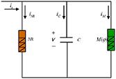
where φ is magnetic flux, v is the voltage across the memristor, and (α, β, γ) denotes the parameters related to the memristor material. Based on equation (116) and Kirchhoff’s law, the current relationship between electronic components in a circuit is described as follows
$\begin{align}{i_M} = - {i_{NR}} - {i_C}.\end{align}$
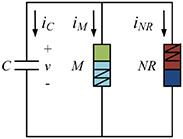
Therefore, the circuit corresponding to the discrete system presented in equation (107) is designed in figure 15.
Figure 15. An MFCM-coupled nonlinear circuit without an inductor. NR is a nonlinear resistor, C denotes a capacitor, and M is an MFCM.
The result in figure 8 illustrates that a map system of a mathematical model is verified by using circuits designed with physical electronic components (a nonlinear resistor, an MFCM, and a capacitor). In fact, the dimension of the dimensionless variables in equation (112) can also be defined by
$\begin{align}w = \frac{{\rho {i_L}}}{{{v_0}}},u = \frac{{q{\rho ^2}}}{{L{v_0}}},\tau = \frac{{\rho t}}{L},\end{align}$
where v0 is the reference voltage, L means the inductance of the induction coil, ρ denotes the resistance of the resistor, and then equation (112) can be updated by
$\begin{equation}\left\{\begin{aligned}L\frac{{{\text{d}}{i_L}}}{{{\text{d}}t}} &= \frac{{{\mu _1^{\prime} }}}{{v_0^2}}\rho {i_L} - \frac{{{\mu _2^{\prime} }}}{{v_0^2}}\frac{{{\rho ^2}i_L^2}}{{{v_0}}} - \frac{{{\rho ^3}c^{\prime}}}{{Lv_0^3}}q{i_L},\\ \frac{{{\text{d}}q}}{{{\text{d}}t}} &= \frac{{b^{\prime}\rho }}{L}q + a^\prime{i_L}.\\ \end{aligned}\right.\end{equation}$
Furthermore, equation (122) is simplified as follows
$\begin{align}\bigg\{ \begin{array}{*{20}{l}} {L\frac{{{\text{d}}{i_L}}}{{{\text{d}}t}} = \eta \rho {i_L} - \varsigma \frac{{{\rho ^2}i_L^2}}{{{v_0}}} - \kappa q{i_L},} \\ {\frac{{{\text{d}}q}}{{{\text{d}}t}} = \delta q + \lambda {i_L},} \end{array}\end{align}$
where
$\begin{align}\eta = \frac{{{\mu _1^{\prime} }}}{{v_0^2}},\varsigma = \frac{{{\mu _2^{\prime} }}}{{v_0^2}},\kappa = \frac{{{\rho ^3}c^{\prime}}}{{Lv_0^3}},\delta = \frac{{b^{\prime}\rho }}{L},\lambda = a^{\prime}.\end{align}$
The higher-order terms in equation (123) are considered as a nonlinear resistor, and it is defined by
$\begin{align}{v_{NR}} = \eta \rho {i_L} - \varsigma \frac{{{\rho ^2}{i_L}^2}}{{{v_0}}},\end{align}$
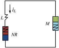
where ρ is the resistance of the nonlinear resistor, (η, ζ) denotes dimensionless parameters of the nonlinear resistor, v0 means the cut-off voltage, and iL is the current across the nonlinear resistor. The nonlinear terms and the second equation in equation (123) are defined as a CCM in the following.
$\begin{equation}\left\{\begin{aligned}{v_M}&=\kappa q{i_L},\\ \frac{{{\text{d}}q}}{{{\text{d}}t}} &= \delta q + \lambda {i_L},\\ \end{aligned}\right.\end{equation}$
where q is charge, iL is the current across the memristor, and (κ, δ, λ) denotes the parameters related to the memristor material. Based on equation (123) and Kirchhoff’s law, the voltage relationship between electronic components in a circuit is described as follows
$\begin{align}{v_L} = {v_{NR}} - {v_M}.\end{align}$
Therefore, the circuit corresponding to the discrete system presented in equation (107) is designed in figure 16.
Figure 16. A CCM-coupled nonlinear circuit without a capacitor. NR is a nonlinear resistor, L means an inductor, and M is a CCM.
A brief summary of the modeling steps of the memristive map based on the memristor-coupled circuit is described as follows:

Step 1: Design a memristor-coupled circuit by connecting and paralleling the memristor with other circuit components.

Step 2: Calculate the output state equation of the memristor-coupled circuit based on Kirchhoff’s laws.

Step 3: Based on the physical dimensions of electronic components, the dimensional calculation of circuit equations is carried out to obtain dimensionless dynamic equations.

Step 4: The dimensionless dynamic equation is transformed linearly to obtain the corresponding map model.

Similarly, the physical verification steps of the chaotic map based on the memristor-coupled circuit are described as follows:

Step 1: Based on the physical quantities and mathematical models of the circuit components, the map equations are dimensionally transformed to obtain the corresponding differential equation forms.

Step 2: Simplify the form of the differential equation obtained in the first step.

Step 3: The differential equation is transformed into a reasonable corresponding mathematical model of electronic components.

Step 4: Based on Kirchhoff’s laws and the results obtained in the third step, a reasonable physical circuit for the electronic components can be designed.

5. Open problems

(1) The map model obtained based on the memristor-coupled circuit does not exhibit hyperchaotic behavior. Establishing hyperchaotic memristor maps or neuron maps based on memristor coupling circuits is an open research topic.
Potential physical and mathematical causes: The generation of hyperchaos requires that the system’s phase space has sufficient dimensions to extend and fold the trajectory. Although the introduction of discrete memristors can increase the mathematical dimension of the mapping, this coupling method does not always effectively generate exponential divergence simultaneously in multiple directions. Some coupling methods may merely ‘project’ chaotic behavior onto new dimensions rather than generating independent chaotic oscillations in multiple dimensions. For instance, simple substitution or series connection of memristors may not be sufficient to create the complex phase space structure required for multiple positive Lyapunov exponents.
(2) The two-dimensional map system has been physically verified by the memristor-coupled circuit. The memristor-coupled circuits of three-dimensional or higher-dimensional map models have been confirmed to be an open research field.
Key implementation challenges: Converting three-dimensional or higher-dimensional discrete mappings into physical circuits means that nonlinear coupling relationships among multiple state variables need to be precisely implemented. This usually involves a large number of operational amplifiers, analog multipliers, memristor model circuits, and addition/subtraction circuits. As the dimension increases, the complexity of the circuit grows exponentially, leading to a significant increase in power consumption, volume, and cost. At the same time, it puts forward extremely high requirements for the layout and wiring of the circuit board to reduce the influence of parasitic parameters
(3) The memristor-coupled circuit design for chaotic maps, without addressing the circuit implementation of neuron maps. The design of the circuit implementation of neuron maps is an open research direction.
Deep-seated challenges and opportunities: memristors mainly play the role of a ‘coupling device’ that generates and enhances nonlinearity in chaotic mapping. However, to construct a neuron model, the memristor needs to simulate the complex electrochemical behavior of biological neurons, including the transmembrane migration of ions, the generation and propagation of action potentials, the refractory period, and the conversion of multiple discharge modes (such as peak discharge and cluster discharge). This requires that the memristor model not only possess nonlinearity but also have complex internal dynamics and multi-time-scale characteristics, which poses higher demands on device physics and materials science.

6. Conclusions

This review provides systematic theoretical and methodological support for solving the problem of converting between the two types of systems based on electronic components by establishing a bidirectional design framework between continuous and discrete nonlinear systems. Research shows that the dynamics of continuous circuits, such as memristor oscillators, can be precisely reduced to discrete mapping models through modeling, and the connection topology of circuit components directly determines the dynamic form of the discrete system. Conversely, the iterative equation of the target discrete system can also be physically implemented through a modular circuit structure, thereby supporting reverse design from the computational model to the hardware system. This framework not only profoundly reveals the intrinsic connection between continuous and discrete dynamics in nonlinear circuits but also provides an extensible methodological foundation for the design of dedicated nonlinear hardware systems for applications such as secure communication, true random number generation, and brain-like computing.

Data availability

No any data are used.

Conflict of interest

The authors declare no conflict of interest with this publication.

Authorship contribution statement

Feifei Yang: Writing-original draft, Methodology, Writing-final version. Xinlin Song: Supervision, Methodology. Ge Zhang: Methodology. Huiping Yin: Supervision, Funding acquisition. Jiangxing Chen: Supervision.

This study is supported by the National Natural Science Foundation of China (62301416), and thanks for Professor Jun Ma guidance on this work.

1
Chua L 2003 Memristor-the missing circuit element IEEE Trans. Circuit Theory 18 507 519

DOI

2
Strukov D B, Snider G S, Stewart D R, Williams R S 2008 The missing memristor found Nature 453 80 103

DOI

3
Muthuswamy B, Kokate P P 2009 Memristor-based chaotic circuits IETE Tech. Rev. 26 417 429

DOI

4
Bao B, Ma Z, Xu J, Liu Z, Xu Q 2011 A simple memristor chaotic circuit with complex dynamics Int. J. Bifurcation Chaos 21 2629 2645

DOI

5
Wu R, Wang C 2016 A new simple chaotic circuit based on memristor Int. J. Bifurcation Chaos 26 1650145

DOI

6
Ma X, Mou J, Liu J, Ma C, Yang F, Zhao X 2020 A novel simple chaotic circuit based on memristor–memcapacitor Nonlinear Dyn. 100 2859 2876

DOI

7
Jin P 2017 A locally active memristor and its application in a chaotic circuit IEEE Trans. Circuits Syst. II 65 246 250

DOI

8
Guo Q, Wang N, Zhang G 2021 A novel current-controlled memristor-based chaotic circuit Integration 80 20 108

DOI

9
Han Z, Al-barakati A A, Jahanshahi H, Mou J 2024 A novel circuit based on memristor-memcapacitor with extreme multistability Nonlinear Dyn. 112 4863 4877

DOI

10
Ding D, Xu X, Yang Z, Zhang H, Zhu H, Liu T 2024 Extreme multistability of fractional-order hyperchaotic system based on dual memristors and its implementation Chaos Solitons Fractals 183 114878

DOI

11
Qi A, Muhammad K, Liu S 2021 Dynamical analysis of the meminductor-based chaotic system with hidden attractor Fractals 29 2140020

DOI

12
Chen M, Li M, Yu Q, Bao B, Xu Q, Wang J 2015 Dynamics of self-excited attractors and hidden attractors in generalized memristor-based Chua’s circuit Nonlinear Dyn. 81 215 226

DOI

13
Chang H, Li Y, Yuan F, Chen G 2019 Extreme multistability with hidden attractors in a simplest memristor-based circuit Int. J. Bifurcation Chaos 29 1950086

DOI

14
Alombah N H, Fotsin H, Romanic K 2017 Coexistence of multiple attractors, metastable chaos and bursting oscillations in a multiscroll memristive chaotic circuit Int. J. Bifurcation Chaos 27 1750067

DOI

15
Wang N, Zhang G, Bao H 2019 Bursting oscillations and coexisting attractors in a simple memristor-capacitor-based chaotic circuit Nonlinear Dyn. 97 1477 1494

DOI

16
Njitacke Z T, kengne J, Fotsin H B, Negou A N, Tchiotsop D 2016 Coexistence of multiple attractors and crisis route to chaos in a novel memristive diode bidge-based Jerk circuit Chaos Solitons Fractals 91 180 197

DOI

17
Bao B C, Bao H, Wang N, Chen M, Xu Q 2017 Hidden extreme multistability in memristive hyperchaotic system Chaos Solitons Fractals 94 102 111

DOI

18
Li Y, Wang M, Chang H, Wang H, Chen G 2024 A hyperchaotic memristive system with extreme multistability and conservativeness Nonlinear Dyn. 112 3851 3868

DOI

19
Prousalis D A, Volos C K, Stouboulos I N, Kyprianidis I M 2017 Hyperchaotic memristive system with hidden attractors and its adaptive control scheme Nonlinear Dyn. 90 1681 1694

DOI

20
Saha P, Saha D C, Ray A, Chowdhury A R 2015 Memristive non-linear system and hidden attractor Eur. Phys. J. Spec. Top. 224 1563 1574

DOI

21
Kengne L K, Muni S S, Chedjou J C, Kyandoghere K 2022 Various coexisting attractors, asymmetry analysis and multistability control in a 3D memristive jerk system Eur. Phys. J. Plus 137 848

DOI

22
Yu F, Zhang W, Xiao X, Yao W, Cai S, Zhang J, Wang C, Li Y 2024 Dynamic analysis and field-programmable gate array implementation of a 5D fractional-order memristive hyperchaotic system with multiple coexisting attractors Fractal Fractional 8 271

DOI

23
Zhao B, Xu S, Wang G 2024 Coexistence of hidden attractors in memristive chaotic system Phys. Scr. 99 125203

DOI

24
Wang M, Deng Y, Liao X, Li Z, Ma M, Zeng Y 2019 Dynamics and circuit implementation of a four-wing memristive chaotic system with attractor rotation Int. J. Non-Linear Mech. 111 149 159

DOI

25
Yan S, Ren Y, Song Z, Shi W, Sun X 2022 A memristive chaotic system with rich dynamical behavior and circuit implementation Integration 85 63 75

DOI

26
Xiu C, Fang J, Ma X 2022 Design and circuit implementations of multimemristive hyperchaotic system Chaos Solitons Fractals 161 112409

DOI

27
Tayyab M, Sun K, Yao Z, Wang H 2024 Dynamics of memristive Liu system and its DSP implementation Phys. Scr. 99 085273

DOI

28
Guo Z, Wen J, Mou J 2022 Dynamic analysis and DSP implementation of memristor chaotic systems with multiple forms of hidden attractors Mathematics 11 24

DOI

29
Dong C, Yang M 2024 A novel 4D memristor-based hyperchaotic system with hidden attractors: dynamics, periodic orbits analysis, and DSP realization Chin. J. Phys. 89 930 942

DOI

30
Sun S, Yan D, Ji’e M, Du X, Wang L, Duan S 2021 Memristor-based time-delay chaotic system with hidden extreme multi-stability and pseudo-random sequence generator Eur. Phys. J. Spec. Top. 230 3481 3491

DOI

31
Chamgoué A C, Sriram S, Kuate P D K, Kingni S T, Rajagopal K 2023 Pseudo random number generator based on memristive Helmholtz snap oscillator with two lines of equilibria embedded in microcontroller Phys. Scr. 98 055213

DOI

32
Chen X, Qian S, Yu F, Zhang Z, Shen H, Huang Y, Cai S, Deng Z, Li Y, Du S 2020 Pseudorandom number generator based on three kinds of four‐wing memristive hyperchaotic system and its application in image encryption Complexity 2020 8274685

DOI

33
Xiong L, Yang F, Mou J, An X, Zhang X 2022 A memristive system and its applications in red–blue 3D glasses and image encryption algorithm with DNA variation Nonlinear Dyn. 107 2911 2933

DOI

34
Liu X, Wang P, Tang D, Tian J 2024 A new four-dimensional memristive system, synchronization and its application in image encryption Int. J. Dyn. Control 12 3669 3684

DOI

35
Rahman Z-A S-A, Jasim B H, Al-yasir Y I A, Abd-alhameed R A 2021 High-security image encryption based on a novel simple fractional-order memristive chaotic system with a single unstable equilibrium point Electronics 10 3130

DOI

36
Xie Y, Ye Z, Li X, Wang X, Jia Y 2024 A novel memristive neuron model and its energy characteristics Cogn. Neurodyn. 18 1989 2001

DOI

37
Yang F, Han Z, Ren G, Guo Q, Ma J 2024 Enhance controllability of a memristive neuron under magnetic field and circuit approach Eur. Phys. J. Plus 139 534

DOI

38
Yang F, Xu Y, Ma J 2023 A memristive neuron and its adaptability to external electric field Chaos Interdiscip. J. Nonlinear Sci. 33 023110

DOI

39
Yang F, Ren G, Tang J 2023 Dynamics in a memristive neuron under an electromagnetic field Nonlinear Dyn. 111 21917 21939

DOI

40
Song X, Yang F 2025 Analysis of electrical activities in a functional neuron with dual memristors J. Theor. Biol. 599 112034

DOI

41
Guo Y, Wu F, Yang F, Ma J 2023 Physical approach of a neuron model with memristive membranes Chaos Interdiscip. J. Nonlinear Sci. 33 113106

DOI

42
Yang F, Song X, Yu Z 2024 Dynamics of a functional neuron model with double membranes Chaos Solitons Fractals 188 115496

DOI

43
Wan J Dynamics and synchronization of neural models with memristive membranes under energy coupling Chin. Phys. B 2024 33 050504 In Chinese)

DOI

44
Yang F, Song X, Yu Z 2025 Adaptive mode selection of electrical activities in a neuron with a memristive ion channel Nonlinear Dyn. 113 7213 7222

DOI

45
Yu Z, Zhu K, Wang Y, Yang F 2025 Dynamics of a neuron with a hybrid memristive ion channel Chaos Solitons Fractals 194 116233

DOI

46
Yang F, Song X, Xu Y 2025 A photocurrent-driven memristive ion channel neuron Chaos Solitons Fractals 199 116740

DOI

47
Tan Y, Wang C 2020 A simple locally active memristor and its application in HR neurons Chaos Interdiscip. J. Nonlinear Sci. 30 053118

DOI

48
Gao Y, Li C, Cen X, Zhang X, Xu J 2025 Firing pattern modification in the FHN neuron via a flux-controlled memristor Chin. J. Phys. 95 1185 1301

DOI

49
Shao Y, Wu F, Wang Q 2024 Synchronization and complex dynamics in locally active threshold memristive neurons with chemical synapses Nonlinear Dyn. 112 13483 13902

DOI

50
Wu F, Kang T, Shao Y, Wang Q 2023 Stability of Hopfield neural network with resistive and magnetic coupling Chaos Solitons Fractals 172 113569

DOI

51
Xu Q 2023 Locally active memristor-based neuromorphic circuit: firing pattern and hardware experiment IEEE Trans. Circuits Syst. I 70 3130 3141

DOI

52
Shi S, Liang Y, Li Y, Lu Z, Dong Y 2024 A neuron circuit based on memristor and negative capacitor: dynamics analysis and hardware implementation Chaos Solitons Fractals 180 114534

DOI

53
Cao H, Cao Y, Qin L, Mou J 2025 Dynamical analysis, multi-cavity control and DSP implementation of a novel memristive autapse neuron model emulating brain behaviors Chaos Solitons Fractals 191 115857

DOI

54
Feali M S 2024 Realization of a pseudo-random number generator utilizing two coupled Izhikevich neurons on an FPGA platform Analog Integr. Circuits Signal Process. 119 57 68

DOI

55
Lai Q, Lai C, Zhang H, Li C 2022 Hidden coexisting hyperchaos of new memristive neuron model and its application in image encryption Chaos Solitons Fractals 158 112017

DOI

56
Lin H, Wang C, Hong Q, Sun Y 2020 A multi-stable memristor and its application in a neural network IEEE Trans. Circuits Syst. II 67 3472 3506

DOI

57
Bao B, Qian H, Xu Q, Chen M, Wang J, Yu Y 2017 Coexisting behaviors of asymmetric attractors in hyperbolic-type memristor based Hopfield neural network Front. Comput. Neurosci. 11 81

DOI

58
Yu F, Wu C, Lin Y, He S, Yao W, Cai S, Jin J 2024 Dynamic analysis and hardware implementation of multi-scroll Hopfield neural networks with three different memristor synapses Nonlinear Dyn. 112 12393 12709

DOI

59
Yang F, Ma J, Wu F 2024 Review on memristor application in neural circuit and network Chaos Solitons Fractals 187 115361

DOI

60
Lin H, Wang C, Deng Q, Xu C, Deng Z, Zhou C 2021 Review on chaotic dynamics of memristive neuron and neural network Nonlinear Dyn. 106 959 973

DOI

61
Xie J, Liu B, Liu X 2026 Delay-embedded reservoir computing with single memristor for scale-efficient temporal signal processing Chaos Solitons Fractals 205 117842

DOI

62
Xie J, Liu B 2026 Hybrid residual reservoir computing using dynamic memristor for time series prediction Chaos Solitons Fractals 205 117866

DOI

63
Xiang Q, Shen Y, Peng S, Liu M 2024 A two-dimensional discrete memristor map: analysis and implementation Int. J. Bifurcation Chaos 34 2450124

DOI

64
Gao S, Iu H H-C, Erkan U, Simsek C, Toktas A, Cao Y, Wu R, Mou J, Li Q, Wang C 2025 A 3D memristive cubic map with dual discrete memristors: design, implementation, and application in image encryption IEEE Trans. Circuits Syst. Video Technol. 35 7706 7718

DOI

65
Peng Y, He S, Sun K 2021 A higher dimensional chaotic map with discrete memristor AEU-Int. J. Electron. Commun. 129 153539

DOI

66
Lai Q, Yang L, Liu Y 2022 Design and realization of discrete memristive hyperchaotic map with application in image encryption Chaos Solitons Fractals 165 112781

DOI

67
Bao H, Hua Z, Li H, Chen M, Bao B 2021 Discrete memristor hyperchaotic maps IEEE Trans. Circuits Syst. I 68 4534 4544

DOI

68
Lai Q, Yang L, Chen G 2023 Design and performance analysis of discrete memristive hyperchaotic systems with stuffed cube attractors and ultraboosting behaviors IEEE Trans. Ind. Electron. 71 7819 7828

DOI

69
Deng Q 2025 Delay difference feedback memristive map: dynamics, hardware implementation, and application in path planning IEEE Trans. Circuits Syst. I 72 7993 8003

DOI

70
Ma Y, Mou J, Jahanshahi H, Alkhateeb A F, Bi X 2023 Design and DSP implementation of a hyperchaotic map with infinite coexisting attractors and intermittent chaos based on a novel locally active memcapacitor Chaos Solitons Fractals 173 113708

DOI

71
Deng Q, Wang C, Sun Y, Yang G 2025 Discrete memristive conservative chaotic map: dynamics, hardware implementation, and application in secure communication IEEE Trans. Cybern. 55 3926 3934

DOI

72
Vijayakumar M, Ahilan A 2024 An optimized chaotic S-box for real-time image encryption scheme based on 4-dimensional memristive hyperchaotic map Ain Shams Eng. J. 15 102620

DOI

73
Wang M, Yi Z, Li Z 2025 A memristive Ikeda map and its application in image encryption Chaos Solitons Fractals 190 115740

DOI

74
Cao Y, Li Z, He S 2024 Complex hidden dynamics in a memristive map with delta connection and its application in image encryption Nonlinear Dyn. 112 7597 8113

DOI

75
Xu Q, Huang L, Wang N, Bao H, Wu H, Chen M 2023 Initial-offset-boosted coexisting hyperchaos in a 2D memristive Chialvo neuron map and its application in image encryption Nonlinear Dyn. 111 20447 20463

DOI

76
Wang Z 2024 Synchronization patterns in a network of diffusively delay-coupled memristive Chialvo neuron map Phys. Lett. A 514 129607

DOI

77
Mehrabbeik M 2021 Synchronization and chimera states in the network of electrochemically coupled memristive Rulkov neuron maps Math. Biosci. Eng. 18 9394 9709

DOI

78
Ma T, Mou J, Chen W 2025 Enriched dynamical behavior of a novel locally active memristor-driven neuron map Chaos Solitons Fractals 198 116537

DOI

79
Ramakrishnan B, Mehrabbeik M, Parastesh F, Rajagopal K, Jafari S 2022 A new memristive neuron map model and its network’s dynamics under electrochemical coupling Electronics 11 153

DOI

80
Zhou X, Sun K, Wang H, Yao Z 2024 Coexisting hyperchaos and multistability in a discrete memristor-coupled bi-neuron model Nonlinear Dyn. 112 9547 9561

DOI

81
Zhang H 2023 A self-rectifying synaptic memristor array with ultrahigh weight potentiation linearity for a self-organizing-map neural network Nano Lett. 23 3107 3115

DOI

82
Cao H, Wang Y, Banerjee S, Cao Y, Mou J 2024 A discrete Chialvo–Rulkov neuron network coupled with a novel memristor model: design, dynamical analysis, DSP implementation and its application Chaos Solitons Fractals 179 114466

DOI

83
Deng W, Ma M 2024 Analysis of the dynamical behavior of discrete memristor-coupled scale-free neural networks Chin. J. Phys. 91 966 976

DOI

84
Guo Y T, Ma J, Zhang X F, Hu X 2024 Memristive oscillator to memristive map, energy characteristic Sci. China Technol. Sci. 67 1567 1578

DOI

85
Ma J 2024 Energy function for some maps and nonlinear oscillators Appl. Math. Comput. 463 128379

DOI

86
Yang F, Ren L, Ma J, Zhu Z 2024 Two simple memristive maps with adaptive energy regulation and digital signal process verification J. Zhejiang Univ. Sci. A 25 394

DOI

87
Yang F, Zhou P, Ma J 2024 An adaptive energy regulation in a memristive map linearized from circuit with two memristive channels Commun. Theor. Phys. 76 035004

DOI

88
Yu Z, He J, Song X, Yang F 2025 Dynamical behaviors of a controllable memristive chaotic map Eur. Phys. J. Plus 140 405

DOI

89
Jia J, Wang C, Zhang X, Zhu Z 2024 Energy and self-adaption in a memristive map neuron Chaos Solitons Fractals 182 114738

DOI

90
Li Y, Lv M, Ma J, Hu X 2024 A discrete memristive neuron and its adaptive dynamics Nonlinear Dyn. 112 7541 7553

DOI

91
Song X, Wang Y, Yang F 2025 A map neuron with a hybrid ion channel and its dynamics Commun. Theor. Phys. 77 085801

DOI

92
Yang F, Song X, Ma J 2024 A memristive map neuron under noisy electric field Chin. J. Phys. 91 287 298

DOI

93
Guo Q, Ren G, Wang C, Zhu Z 2025 Reliability and energy function of an oscillator and map neuron BioSystems 251 105443

DOI

94
Chen Y, Yang F, Wang C 2025 Coherence reson-ance in a memristive map neuron and adaptive energy regulation Mod. Phys. Lett. B 39 2550008

DOI

95
Li Y, Guo Q, Wang C, Ma J 2024 A map neuron with piezoelectric membrane, energy regulation and coherence resonance Commun. Nonlinear Sci. Numer. Simul. 139 108320

DOI

96
Wang B, Zhang X, Zhu Z, Ren G 2024 A new memristive map neuron, self-regulation and coherence resonance Eur. Phys. J. B 97 124

DOI

97
Lei Z, Ma J 2025 Coherence resonance and energy dynamics in a memristive map neuron Chaos Interdiscip. J. Nonlinear Sci. 35 023158

DOI

98
Yang F, Song X, He J, Yin H 2026 Design and energy function determination of a memristor-coupled circuit representing a two-dimensional chaotic map J. Zhejiang Univ. Sci. A 27 76 86

DOI

Outlines

/