We investigate exact soliton solutions, bifurcation structures, and chaotic behavior in the Akbota-Myrzakulov-Tolkynay-Zhaidary (AMTZ) equation, which governs nonlinear wave propagation in multi-dimensional dispersive systems. Using the improved modified Sardar sub-equation method, we develop hyperbolic, trigonometric, and rational function solutions, along with full visualizations illustrating wave stability characteristics. Bifurcation analysis yields critical equilibrium points such as saddle, center, and cuspidal configurations, and phase portraits reveal complicated nonlinear transitions. Adding external periodic perturbations reveals chaotic attractors confirmed using Poincaré sections and positive Lyapunov exponents, establishing sensitivity to initial conditions. The AMTZ equation is used extensively in the field of optical fiber communications, plasma physics, and fluid dynamics. This is the first comprehensive chaos analysis of the AMTZ equation, connecting exact soliton construction with nonlinear dynamical characterization, providing a theoretical framework for modeling and controlling nonlinear wave processes across disciplines.
Salim S Mahmood, Muhammad Amin S Murad. Investigation of the soliton solutions, bifurcation analysis, and chaotic nature of the Akbota-Myrzakulov-Tolkynay- Zhaidary equation[J]. Communications in Theoretical Physics, 2026, 78(8): 085002. DOI: 10.1088/1572-9494/ae6a79
1. Introduction
Nonlinear partial differential equations (NPDEs) are fundamental mathematical models for describing complex phenomena in various branches of science, including fluid dynamics, plasma physics, optical communications, and quantum mechanics [1]. Optical solitons are self-reinforcing solitary wave packets that maintain their shape and velocity during propagation due to a precise balance between nonlinear self-phase modulation and linear group velocity dispersion [2]. In optical fiber systems, bright solitons form when anomalous dispersion compensates Kerr nonlinearity, while dark solitons intensity dips on a continuous wave background-arise in the normal dispersion regime.
Bifurcation theory is the mathematical study of qualitative changes in the structure of the phase portrait of a dynamical system as one or more parameters vary continuously [3]. In the context of nonlinear wave equations, bifurcation analysis identifies critical parameter values at which the number or stability of equilibrium points changes, revealing qualitative transitions such as the emergence of periodic orbits or the merging of equilibria. The natural nonlinear and dispersive nature of these models enable the generation of localized wave structures, called solitons, that keep their shape and velocity during propagation and collision processes [4]. Recently, much research has been done, establishing powerful analytical and numerical techniques to discover exact solutions to NPDEs such as the inverse scattering transform [5], the bilinear method proposed by Hirota [6], Bácklund transformations [7], Darboux transformations [8], the extended tanh-function method [9], the Exp-function method [10], $(G^{^{\prime}}/G)$-expansion method [11], modified Kudryashov method [12] and Sardar sub-equation method [13]. The nonlinear Schrödinger equation (NLSE) and its variants are among the various classes of NPDEs, and they have received a lot of interest lately, on account of their central relevance for describing the evolution of a wave packet in a dispersive medium [14]. The NLSE for pulse propagation in optical fibers is determined by dispersion, where balance between dispersion and nonlinearity cause soliton formation [15]. Numerous general forms of the Schrödinger equation have been investigated, for example, cubic-quintic NLSE [16], higher-order NLSE with fourth-order dispersion [17], derivative NLSE [18], coupled NLSE systems [19], as well as space-time fractional NLSE [20], amongst others. Soliton solutions have been generated by employing various sophisticated methods from these models, such as the modified simple equation method [21], the new extended direct algebraic method [22], the unified Riccati equation expansion method [23], and the generalized exponential rational function method [24]. In the case of multi-dimensional wave propagation phenomena, integrable systems with (2+1)-dimensional structures have been of considerable importance in modeling transverse perturbations and instabilities [25]. Originally intended to characterize the nonlinear spin dynamics for ferromagnetics, the Myrzakulov family of equations has been used in both nonlinear optics as well as in plasma physics [26]. The previous studies on Myrzakulov-type equations and their solution structure have greatly improved. Kumar et al [27] studied the Myrzakulov-I equation using the modified exp-function method and identified numerous soliton families. Rezazadeh et al [28] proposed the new Kudryashov method on the Myrzakulov-II equation, and obtained hyperbolic and trigonometric function solutions. Ali and Mehanna [29] successfully used the unified method to extract optical solitons from the Myrzakulov-III equation resulting in bright, dark, and singular soliton propagation. As a newly proposed integrable (2+1)-dimensional model we extend the classical Myrzakulov framework through Akbota-Myrzakulov-Tolkynay-Zhaidary (AMTZ) equation. The AMTZ system can be illustrated with the following coupled NPDEs [30, 31]:
$\Pi_{t}-\frac{X \Pi_{x}}{b}+\frac{\beta \Pi \Omega_{y}}{b}-\frac{\beta \Omega_{x x y}}{4 a b}=0,$
$X_{x}+\frac{\beta \Omega_{y}}{2}=0,$
where $\Omega(x,y,t)$ is the primary wave amplitude function, $\Pi(x,y,t)$ is the auxiliary wave function and $X(x,y,t)$ is a potential function. Our independent variables are $x$ and $y$ (space coordinates) and $t$ (temporal variable). The parameter $\beta$ is the nonlinearity coefficient related to the amplitude of self-phase modulation and cross-phase modulation effects, $b$ is a characteristic scaling factor associated with spatial dimensions and properties of materials, and $a$ is considered the intensity of higher-order dispersive effects. In equation (1), the temporal derivative $\Omega_t$ expresses the temporal evolution, the advection parameter $-X\Omega_x/b$ describes the transport influenced by the potential field, the nonlinear parameter $\beta\Omega\Omega_y/b$ indicates the transverse modulation, and $\beta\Pi_y$ denotes the coupling between fields. In equation (2), the higher-order dispersion term $\beta\Omega_{xxy}/(4ab)$ creates mixed derivative effects combining longitudinal and transverse differences. The constraint equation (3) establishes an integral connection between $X$ and $\Omega$. In spite of its mathematical framework and practical usage in electromagnetic wave propagation and magneto-acoustic wave dynamics [32], the AMTZ equation has never been much studied. Mathanaranjan and Myrzakulov [31] established its Lax pair representation to validate integrability and did not present explicit analytical solutions. Myrzakulov et al [30] have presented the AMTZ system in integrable spin models but did not examine solutions comprehensively. More advanced solution approaches have shown promise in solving similar models recently. Bin et al [33] used modified extended tanh expansion for coupled dispersive systems. Alquran [34] applied the sine-Gordon expansion method for (2+1)-dimensional equations. Raza et al [35] used unified Riccati equation technique for intricate Ginzburg-Landau equations. Unfortunately, the previous studies concentrated mainly on solution generation rather than dynamical system structure. Kamel et al have proposed an improved modified Sardar sub-equation method (IMSSEM) [36], which allows us to take on greater flexibility as the auxiliary equation $G^{^{\prime} 2}(\xi) = C G^4(\xi) + B G^2(\xi) + A$ allows us to derive larger solution families. This provides a valuable insight for assessing the stability of a network [37]. Bifurcation analysis investigates how equilibrium structures shift with parameter variations [38]. Chu et al [39] studied bifurcation phenomenon in Boussinesq equation. Jhangeer et al [40] studied chaos of perturbed NLSEs through the use of Lyapunov exponents and Poincaré sections. Nevertheless, despite these developments, no study has studied the dynamic behavior of bifurcation structures and chaotic dynamics in the AMTZ equation. The motivation to investigate the AMTZ equation derives from its application in multi-mode fiber communications, pulse dynamics in the context of dispersive optical systems, as well as wave propagation phenomena [39, 41-45]. However, a number of pressing research gaps persist: no systematic classification of exact analytical solutions has been established for the AMTZ system; relationship between model parameters and solution properties has not been established; phase plane analysis and equilibrium systems have not yet been investigated; the system's external periodic forcing response has not yet been considered; and it remains unstructured to compare the presented approaches with the existing solution methods demonstrating that the IMSSEM provides the advantages. The challenges and limitations identified in previous research could be addressed through a systematic method of constructing exact soliton solutions using the improved modified simple equation method, bifurcation analysis through the use of equilibrium point classification and phase portrait building, chaotic dynamics studies regarding periodic perturbations, validated by Lyapunov exponents, and solutions stability characterization through the analysis of temporal evolution, and physical implications for applications in nonlinear optics and plasma physics. The novelty of this work is threefold. First, this is the first study to apply the IMSSEM to the AMTZ equation, generating seventeen distinct exact solution families (hyperbolic, trigonometric, and rational) in a single unified framework a scope that surpasses all prior analytical treatments of Myrzakulov-type equations (see table 2). Second, this work presents the first systematic bifurcation analysis and phase portrait construction for the AMTZ system, classifying all equilibrium points and revealing critical parameter thresholds governing qualitative transitions. Third, this is the first study to demonstrate chaotic dynamics in the AMTZ equation via positive Lyapunov exponents and fractal Poincaré sections under external periodic perturbations, establishing that this integrable system possesses rich dynamical complexity when disturbed.
The IMSSEM offers three key advantages over standard methods such as the extended tanh method [46], the $(G^{^{\prime}}/G)$-expansion method [47], and the modified Kudryashov method [48]. (i) Solution diversity: the auxiliary equation $G^{^{\prime} 2} = CG^4 + BG^2 + A$ encodes three independent parameters $(A, B, C)$, allowing simultaneous derivation of rational, hyperbolic, and trigonometric families in a single algebraic system, whereas methods such as $(G^{^{\prime}}/G)$-expansion produce only one family type per run. (ii) Generality: the IMSSEM subsumes several sub-equation methods as special cases (e.g. setting $A = 0$ recovers Sardar sub-equation results), making it strictly more general. (iii) Computational efficiency: the polynomial structure of the method reduces the solution search to a single algebraic system solvable by Maple, avoiding the iterative steps required in numerical or transformation-based methods. The AMTZ scheme can thus accommodate a variety of analytical families via IMSSEM, showing computational efficiency gains compared to traditional approaches. Bifurcation analysis discloses critical transitions of individual parameters and chaos analysis demonstrates that the integrable system is sensitive to external perturbations that can be crucial in applications with real-world effects.
The remainder of the paper is organized as follows. Section 2 introduces the traveling wave transformation that reduces the AMTZ system to an ODE. Section 3 applies the IMSSEM to derive explicit solution families. Section 4 performs bifurcation analysis. Section 5 investigates chaotic dynamics. Section 6 discusses results and physical implications. Section 7 presents conclusions, and section 8 outlines key findings, limitations, and future directions.
2. Description of the transformation
The traveling wave transformation method must be used in order to solve equation (1).
Here, $U(\xi)$, $V(\xi)$, and $R(\xi)$ are real-valued profile functions of the traveling wave coordinate $\xi = px + qy - vt$, where $p$ and $q$ are the wave numbers in the $x$- and $y$-directions, respectively, and $v$ is the wave propagation speed. The functions $\Omega$, $\Pi$, and $X$ depend only on $\xi$ under this reduction, converting the PDE system into a system of ODEs.
The following are obtained by substituting the transformations from equation (4) into equations (1)-(3):
$\begin{align} &\beta U U_{\xi} q +\left(-V p -b v \right) U_{\xi}-\beta R_{\xi} q b = 0, \end{align}$
$\begin{align} &4 \beta R U_{\xi} q a -\beta U_{\xi\xi\xi} q \,p^{2}-4 R_{\xi} a \left(V p +b v \right) = 0, \end{align}$
Integrating equation (7) with respect to $\xi$ and applying the localized wave boundary conditions $U \to 0$ and $V \to 0$ as $|\xi| \to \infty$ (i.e. requiring solutions to vanish at infinity) , the integration constant is set to zero [49-54], yielding
$U=-\frac{2 p V}{\beta q}$
substitute equation (8) into equation (5), we obtain
$-\beta^{2} R_{\xi} q^{2} b+6 p^{2} V V_{\xi}+2 p V_{\xi} v b=0$
Integrating equation (9) and setting the integration constant to zero under the same localized boundary conditions, we obtain
$R=\frac{V p(3 V p+2 b v)}{\beta^{2} q^{2} b}$
Substitute equations (8) and (10) into equation (6), we obtain
$\begin{align} 4 a \left(6 V^{2} p^{2}+6 V b p v +b^{2} v^{2}\right) V_{\xi}-p^{2} V_{\xi\xi\xi} \beta^{2} q^{2} b = 0.\end{align}$
Integrating equation (11) and setting the integration constant to zero under the same localized boundary conditions, we obtain
$\begin{align} -p^{2} \beta^{2} q^{2} b V_{\xi\xi}+4 a V \left(V p +b v \right) \left(b v +2 V p \right) = 0.\end{align}$
We find that the balancing parameter is $N = 1$ by homogeneous balance analysis of equation (12), taking into account the link between the nonlinear term $V^{3}$ and the highest-order derivative term $V_{\xi\xi}$.
3. Application of the IMSSEM
In this section, we apply the IMSSEM to construct novel optical soliton solutions of the governing model. We assume that the solution of equation (12) can be expressed in the finite series form
$V(\xi)=\sum_{i=0}^{N} \delta_{i} G(\xi)^{i}$
where $\delta_{i}$ $(i = 0,1,2,\ldots,N)$ are unknown constants to be determined and $N$ is a positive integer obtained via the homogeneous balance principle. By balancing the highest-order derivative term with the nonlinear term in equation (12), we obtain $N = 1$. Consequently, equation (13) reduces to
$V(\xi)=\delta_{0}+\delta_{1} G(\xi)$
where the auxiliary function $G(\xi)$ satisfies the nonlinear ordinary differential equation
$G_{\xi}^{2}=C G^{4}+B G^{2}+A$
with $A$, $B$, and $C$ being real constants.
Case 1: rational function solutions.
When $A = 0$, $B = 0$, and $C \gt 0$, equation (15) admits rational solutions given by
Substituting equations (14) and (15) into equation (12) yields a polynomial in $G(\xi)^{i}$ $(i = 0,1,\ldots,3)$. By equating the coefficients of like powers of $G(\xi)$ to zero, a system of algebraic equations is obtained. This system is solved using the symbolic computation software Maple 2024 , leading to the determination of the unknown constants.
Result .1
$\begin{align} &a = -\frac{\beta^{2} q^{2} B \,p^{2}}{2 b \,v^{2}}, b = b, \beta = \beta, p = p, q = q, v = v,\nonumber\\ \delta_{0} &= -\frac{b v}{2 p}, \delta_{1} = \frac{\sqrt{-2 B C}\, v b}{2 B p}. \end{align}$
The obtained rational, hyperbolic, and trigonometric solution families together with their corresponding parameter constraints are summarized in table 1.
Table 1. Summary of solution families of the AMTZ equation derived via IMSSEM.
Equation
Type
Function
Constraints
(34)
Rational
Equation (16)
$A = 0,\; B = 0,\; C \gt 0$
(35)
Hyperbolic (cosh/sinh)
Equation (17)
$A = 0,\; B \gt 0,\; C \gt 0$
(36)
Hyperbolic (cosh/sinh)
Equation (18)
$A = 0,\; B \gt 0,\; C \gt 0$
(37)
Hyperbolic (sech)
Equation (19)
$A = 0,\; B \gt 0,\; C\neq 0$
(38)
Hyperbolic (csch)
Equation (20)
$A = 0,\; B \gt 0,\; C\neq 0$
(39)
Hyperbolic (tanh)
Equation (21)
$A = \dfrac{B^2}{4C},\; B \lt 0,\; C \gt 0$
(40)
Hyperbolic (coth)
Equation (22)
$A = \dfrac{B^2}{4C},\; B \lt 0,\; C \gt 0$
(41)
Hyperbolic (tanh + i sech)
Equation (23)
$A = \dfrac{B^2}{4C},\; B \lt 0,\; C \gt 0$
(42)
Hyperbolic (coth + csch)
Equation (24)
$A = \dfrac{B^2}{4C},\; B \lt 0,\; C \gt 0$
(43)
Hyperbolic (tanh + coth)
Equation (25)
$A = \dfrac{B^2}{4C},\; B \lt 0,\; C \gt 0$
(44)
Trigonometric (sec)
Equation (26)
$A = 0,\; B \lt 0,\; C\neq 0$
(45)
Trigonometric (csc)
Equation (27)
$A = 0,\; B \lt 0,\; C\neq 0$
(46)
Trigonometric (tan)
Equation (28)
$A = \dfrac{B^2}{4C},\; B \gt 0,\; C \gt 0$
(47)
Trigonometric (cot)
Equation (29)
$A = \dfrac{B^2}{4C},\; B \gt 0,\; C \gt 0$
(48)
Trigonometric (tan + sec)
Equation (30)
$A = \dfrac{B^2}{4C},\; B \gt 0,\; C \gt 0$
(49)
Trigonometric (cot + csc)
Equation (31)
$A = \dfrac{B^2}{4C},\; B \gt 0,\; C \gt 0$
(50)
Trigonometric (tan $-$ cot)
Equation (32)
$A = \dfrac{B^2}{4C},\; B \gt 0,\; C \gt 0$
Table 2. Comparison of solution types obtained for Myrzakulov-family equations using various methods.
where $Z = \frac{\sqrt{2}\, \sqrt{-B}\, \left(p x +q y -v t +\xi_{0} \right)}{4}$.
From equations (4), (8), (10), (14), (26), and (33), we obtain the following soliton solution:
$\begin{equation} \begin{aligned} &\Omega \! \left(x , y , t\right) = \frac{b v \left(-\sqrt{2}\, \sqrt{-B C}\, \sqrt{-\frac{B}{C}}\, \sec \! \left(\sqrt{-B}\, \left(p x +q y -v t +\xi_{0} \right)\right)+B \right)}{\beta q B},\\&X \! \left(x , y , t\right) = -\frac{b v \left(-\sqrt{2}\, \sqrt{-B C}\, \sqrt{-\frac{B}{C}}\, \sec \! \left(\sqrt{-B}\, \left(p x +q y -v t +\xi_{0} \right)\right)+B \right)}{2 B p},\\&\Pi \! \left(x , y , t\right) = \frac{b \,v^{2} \left(6 B \left(\sec^{2}\left(\sqrt{-B}\, \left(p x +q y -v t +\xi_{0} \right)\right)\right)-2 \sqrt{2}\, \sqrt{-B C}\, \sqrt{-\frac{B}{C}}\, \sec \! \left(\sqrt{-B}\, \left(p x +q y -v t +\xi_{0} \right)\right)-B \right)}{4 \beta^{2} q^{2} B}. \end{aligned}\end{equation}$
From equations (4), (8), (10), (14), (27), and (33), we obtain the following soliton solution:
$\begin{equation} \begin{aligned} &\Omega \! \left(x , y , t\right) = \frac{b v \left(-\sqrt{2}\, \sqrt{-B C}\, \sqrt{-\frac{B}{C}}\, \csc \! \left(\sqrt{-B}\, \left(p x +q y -v t +\xi_{0} \right)\right)+B \right)}{\beta q B},\\&X \! \left(x , y , t\right) = -\frac{b v \left(-\sqrt{2}\, \sqrt{-B C}\, \sqrt{-\frac{B}{C}}\, \csc \! \left(\sqrt{-B}\, \left(p x +q y -v t +\xi_{0} \right)\right)+B \right)}{2 B p},\\&\Pi \! \left(x , y , t\right) = \frac{b \,v^{2} \left(6 B \left(\csc^{2}\left(\sqrt{-B}\, \left(p x +q y -v t +\xi_{0} \right)\right)\right)-2 \sqrt{2}\, \sqrt{-B C}\, \sqrt{-\frac{B}{C}}\, \csc \! \left(\sqrt{-B}\, \left(p x +q y -v t +\xi_{0} \right)\right)-B \right)}{4 \beta^{2} q^{2} B}. \end{aligned}\end{equation}$
From equations (4), (8), (10), (14), (28), and (33), we obtain the following soliton solution:
$\begin{equation} \begin{aligned} &\Omega \! \left(x , y , t\right) = \frac{b v \left(-\sqrt{-B C}\, \sqrt{\frac{B}{C}}\, \tan \! \left(\frac{\sqrt{2}\, \sqrt{B}\, \left(p x +q y -v t +\xi_{0} \right)}{2}\right)+B \right)}{\beta q B},\\&X \! \left(x , y , t\right) = -\frac{b v \left(-\sqrt{-B C}\, \sqrt{\frac{B}{C}}\, \tan \! \left(\frac{\sqrt{2}\, \sqrt{B}\, \left(p x +q y -v t +\xi_{0} \right)}{2}\right)+B \right)}{2 B p},\\&\Pi \! \left(x , y , t\right) = -\frac{b \,v^{2} \left(2 \sqrt{-B C}\, \sqrt{\frac{B}{C}}\, \tan \! \left(\frac{\sqrt{2}\, \sqrt{B}\, \left(p x +q y -v t +\xi_{0} \right)}{2}\right)+3 B \left(\sec^{2}\left(\frac{\sqrt{2}\, \sqrt{B}\, \left(p x +q y -v t +\xi_{0} \right)}{2}\right)\right)-2 B \right)}{4 \beta^{2} q^{2} B}. \end{aligned}\end{equation}$
From equations (4), (8), (10), (14), (29), and (33), we obtain the following soliton solution:
$\begin{equation} \begin{aligned} &\Omega \! \left(x , y , t\right) = \frac{b v \left(-\sqrt{-B C}\, \sqrt{\frac{B}{C}}\, \cot \! \left(\frac{\sqrt{2}\, \sqrt{B}\, \left(p x +q y -v t +\xi_{0} \right)}{2}\right)+B \right)}{\beta q B},\\&X \! \left(x , y , t\right) = -\frac{b v \left(-\sqrt{-B C}\, \sqrt{\frac{B}{C}}\, \cot \! \left(\frac{\sqrt{2}\, \sqrt{B}\, \left(p x +q y -v t +\xi_{0} \right)}{2}\right)+B \right)}{2 p B},\\&\Pi \! \left(x , y , t\right) = -\frac{b \,v^{2} \left(-\sqrt{-B C}\, \sqrt{\frac{B}{C}}\, \cot \! \left(\frac{\sqrt{2}\, \sqrt{B}\, \left(p x +q y -v t +\xi_{0} \right)}{2}\right)+B \right) \left(3 \sqrt{-B C}\, \sqrt{\frac{B}{C}}\, \cot \! \left(\frac{\sqrt{2}\, \sqrt{B}\, \left(p x +q y -v t +\xi_{0} \right)}{2}\right)+B \right)}{4 \beta^{2} q^{2} B^{2}}. \end{aligned}\end{equation}$
From equations (4), (8), (10), (14), (30), and (33), we obtain the following soliton solution:
$\begin{equation} \begin{aligned} &\Omega \! \left(x , y , t\right) = \frac{b v \left(-\sqrt{-B C}\, \sqrt{\frac{B}{C}}\, \tan \! \left(Z \right)-\sqrt{-B C}\, \sqrt{\frac{B}{C}}\, \sec \! \left(Z \right)+B \right)}{\beta q B} ,\\&X \! \left(x , y , t\right) = -\frac{b v \left(-\sqrt{-B C}\, \sqrt{\frac{B}{C}}\, \tan \! \left(Z \right)-\sqrt{-B C}\, \sqrt{\frac{B}{C}}\, \sec \! \left(Z \right)+B \right)}{2 B p},\\&\Pi \! \left(x , y , t\right) = \frac{b \,v^{2} \left(\sqrt{-B C}\, \sqrt{\frac{B}{C}}\, \cos \! \left(\sqrt{2}\, \sqrt{B}\, \left(p x +q y -v t +\xi_{0} \right)\right)+B \left(\sin \! \left(\sqrt{2}\, \sqrt{B}\, \left(p x +q y -v t +\xi_{0} \right)\right)+2\right)\right)}{2 \left(\sin \! \left(\sqrt{2}\, \sqrt{B}\, \left(p x +q y -v t +\xi_{0} \right)\right)-1\right) \beta^{2} q^{2} B}, \end{aligned}\end{equation}$
where $Z = \sqrt{2}\, \sqrt{B}\, \left(p x +q y -v t +\xi_{0} \right)$.
From equations (4), (8), (10), (14), (31), and (33), we obtain the following soliton solution:
where $Z = \frac{\sqrt{2}\, \sqrt{B}\, \left(p x +q y -v t +\xi_{0} \right)}{4}$.
Verification of solutions
To validate the derived solutions, each solution family has been verified by direct back-substitution into both the reduced ODE equation (12) and the original PDE system (1)-(3) using the symbolic computation software Maple 2024. The substitution yields a zero remainder in each case, confirming mathematical consistency. As a representative example, substituting equation (34) into equation (1) via the transformation equation (4) produces identically zero, which validates the result. Similar verifications were performed for all solution families in equations (35)-(50).
4. Bifurcation analysis
Applying the Galilean transformation for equation (12), we obtain the following dynamical system:
$\begin{equation} \begin{cases} V_\xi = \Phi \! \left(\xi \right) b \,\beta^{2} p^{2} q^{2},\\ \Phi_\xi = 4 a \,b^{2} v^{2} V \! \left(\xi \right)+12 a b p v V \! \left(\xi \right)^{2}+8 a \,p^{2} V \! \left(\xi \right)^{3}. \end{cases}\end{equation}$
To find the equilibrium points of system (51), we set $V_\xi = 0$ and $\Phi_\xi = 0$. From the first equation, $\Phi = 0$. Substituting into the second equation gives $4ab^2v^2 V + 12abpv V^2 + 8ap^2 V^3 = 0$, which factors as $4aV(bv + 2pV)(bv + pV) = 0$. This yields three solutions: $V = 0$, $V = -bv/(2p)$, and $V = -bv/p$, giving the equilibrium points
where $S_1 = -\frac{b v}{p}$, $S_2 = -\frac{b v}{2 p}$.
Moreover, this is also the first integral of the system equation (51) which we have used along with the points for phase portrait
$\begin{align} & H\left(V,\Phi\right) \nonumber\\ &\,\, = -\frac{\Phi \! \left(\xi \right)^{2} b \,\beta^{2} p^{2} q^{2}-4 a \,b^{2} v^{2} V \! \left(\xi \right)^{2}-8 a b p v V \! \left(\xi \right)^{3}-4 a \,p^{2} V \! \left(\xi \right)^{4}}{2 b \,\beta^{2} p^{2} q^{2}},\end{align}$
$\begin{align} & \mathcal{J}\left(V,\Phi\right) = \begin{vmatrix} 0 & b \,\beta^{2} p^{2} q^{2} \\ 24 V \! \left(\xi \right)^{2} a \,p^{2}+24 V \! \left(\xi \right) a b p v +4 a \,b^{2} v^{2} & 0 \end{vmatrix}\nonumber\\ &\qquad\qquad = -4 b \,\beta^{2} p^{2} q^{2} a \left(6 V \! \left(\xi \right)^{2} p^{2}+6 V \! \left(\xi \right) b p v +b^{2} v^{2}\right).\end{align}$
Therefore we have the following property:
•
(•)(V,0) denotes saddle if $\mathcal{J}(V,\Phi) \lt 0,$
•
(•)(V,0) indicates center if $\mathcal{J}(V,\Phi) \gt 0,$
•
(•)(V,0) indicates cuspidal if $\mathcal{J}(V,\Phi) = 0$.
Then there are the following different dynamical system cases:
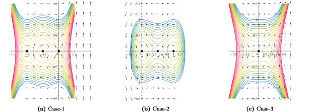
(Case 1:)when $S_1 \lt 0$ and $S_2 \lt 0$ are given by $a = 1, b = 1, \beta = 1, p = 1, q = 1, v = 1$, and with given parameters we recognized EPs, which are $(0,0)$, $(-1,0)$, and $\left(\frac{-1}{2},0\right)$ these EPs are illustrated in figure 11(a) with points $(0,0)$, $(-1,0)$ being saddle points with eigenvalues $\lambda_1 = 2,\lambda_2 = -2$, while $\left(\frac{-1}{2},0\right)$ is center point with eigenvalues $\lambda_1 = \sqrt{-2},\lambda_2 = -\sqrt{-2}$.
(Case 2:)$S_1 \gt 0$ and $S_2 \gt 0$, at some values $a = 1, b = -1, \beta = 1, p = 1, q = 1, v = 1$, we found EPs that are $(0,0)$, $\left(\frac{1}{2},0\right)$, and $(1,0)$ these EPs are given in figure 11(b) pointing to $(0,0)$, $(1,0)$ where $(1,0)$ is a center point with eigenvalues $\lambda_1 = 2i,\lambda_2 = -2i$, while $\left(\frac{1}{2},0\right)$ represents the saddle point with eigenvalues $\lambda_1 = \sqrt{2},\lambda_2 = -\sqrt{2}$.
(Case 3:)if $S_1 = 0$ and $S_2 = 0$, for parameters $a = 1, b = 1, \beta = 1, p = 1, q = 1, v = 0$, EP is $(0,0)$, and this EP is shown in figure 11(c) with point $(0,0)$ as a cuspidal point.
5. Chaotic analysis
Chaotic behavior in nonlinear dynamical systems is a fundamental phenomenon showing extreme sensitivity to initial conditions [40]. The perturbed dynamical system studied is equation (55), where the unperturbed Hamiltonian system (51) is forced by the periodic term $\epsilon\cos(\theta\xi)$. This perturbation breaks the Hamiltonian structure and can induce chaotic motion via homoclinic/heteroclinic orbit intersections near saddle equilibria (Melnikov theory). Numerical integration is performed using the Runge-Kutta 4th-order (RK4) method with step size $h = 0.001$ and absolute/relative tolerance $10^{-8}$ over the interval $\xi \in [0, 300]$. The Lyapunov exponents are computed using the standard Gram-Schmidt orthonormalization algorithm [55]: two tangent vectors are evolved alongside the trajectory, and at each step their lengths are recorded and the vectors re-orthonormalized; the Lyapunov exponents are the time-averaged logarithms of the successive expansion factors. A positive largest exponent $\lambda_1 \gt 0$ confirms chaos. Initial conditions and forcing parameters for each case are specified in the captions of figures 6-8.
It is important to distinguish between the unperturbed ($\epsilon = 0$) and perturbed ($\epsilon \neq 0$) cases. When $\epsilon = 0$, system (51) is a Hamiltonian (integrable) system with conserved energy $H(V,\Phi)$ given by equation (53), and all trajectories are either periodic orbits (around center points) or heteroclinic/homoclinic connections (near saddle points). No chaos is possible in the unperturbed case, as the phase space is entirely organized by these invariant structures. When $\epsilon \neq 0$, the periodic external forcing $\epsilon\cos(\theta\xi)$ breaks the Hamiltonian structure and can cause homoclinic orbit splitting, leading to the formation of chaotic layers around the formerly ordered saddle connections. This is the mechanism by which disorder (chaos) arises: the addition of even a small external periodic disturbance can destroy the integrability and produce exponential sensitivity to initial conditions, as confirmed by the positive Lyapunov exponents in figure 8. To investigate the emergence of chaos in the AMTZ equation, we introduce an external periodic forcing term into the dynamical system derived in section 4. The perturbed system is expressed as
$\begin{align} \begin{cases} V_\xi = \Phi \! \left(\xi \right) b \,\beta^{2} p^{2} q^{2},\\ \Phi_\xi = 4 a \,b^{2} v^{2} V \! \left(\xi \right)+12 a b p v V \! \left(\xi \right)^{2}+8 a \,p^{2} V \! \left(\xi \right)^{3}+ \epsilon\cos\left(\theta\xi\right), \end{cases}\end{align}$
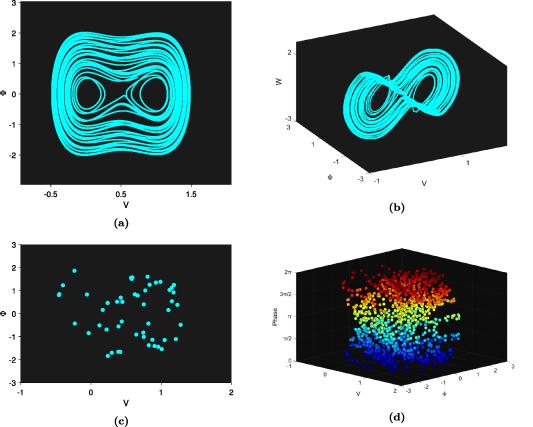
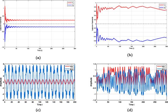
where $\epsilon$ in turn is the amplitude of the external perturbation and $\theta$ is the forcing frequency. This perturbation mimics realistic environmental disturbances in experiments [39]. Lyapunov exponents, as quantitative measures of chaotic dynamics, measure the average rate of divergence or convergence in phase space of neighboring trajectories [37]. For example, a positive largest Lyapunov exponent $\lambda_1 \gt 0$ indicates that the behavior of the dynamics may be chaotic and highly sensitive to the initial condition, $\lambda_1 = 0$ is indicative of periodic or quasi-periodic motion, and $\lambda_1 \lt 0$ denoting asymptotic stability. Numerical integration techniques are used to compute the time-dependent Lyapunov exponents. The Poincaré section presents a geometric visualization method for studying dynamic systems, as it involves sampling trajectories at regular intervals in the phase space [38]. For periodic orbits, the Poincaré section is comprised of discrete points, while chaotic attractors are fractal structures with complex patterns. Multi-stability analysis demonstrates how multiple attractors maintain the same initial characteristics under different, though identical, parameters, showing the sensitivity of the system to initial conditions. The chaotic behavior, phase portraits, Poincaré sections, Lyapunov exponents, and multi-stability plots of the systems for distinct parameter sets is shown in figures 6-8, showing that the AMTZ system shows strong chaotic dynamics during external periodic perturbations.
6. Results and discussion
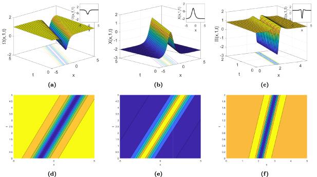
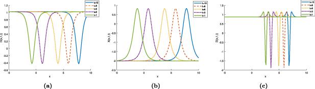
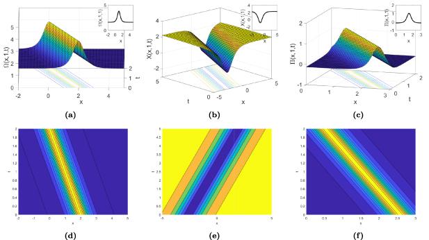
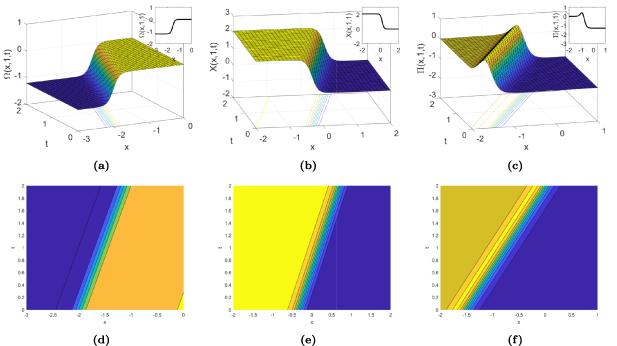
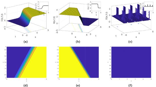
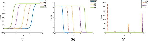
After implementing the IMSSEM, it has shown that it is the most satisfactory method to obtain seventeen true analytical solution families from the AMTZ equation. And it also found a complete and diverse data of seventeen exact analytical product families across hyperbolic, trigonometric, rational function types. Direct back-substitution of the reduced ODE equation (12) (substitution into both PDE (1)-(3)) results in a pure 0 difference returned by mathematical computation software Maple 2024 in every case. These solutions capture specific nonlinear wave phenomena in multi-dimensional dispersive systems, which are highly relevant to the future field of optical fiber communication, plasma physics, and fluid dynamics. Figure 1 gives rise to 3D surface and 2D contour plots of the soliton solutions calculated in equation (35) that is a member of the hyperbolic cosh/sinh family. Figure 1(a) is the result of a bright soliton structure with focused amplitude peak and is propagated through the spatial domain. This corresponds to, in a physical meaning, the optical energy level in a fiber waveguide with the Kerr nonlinearity effectively offsetting the group-velocity dispersion and generating a self-sustaining pulse. The bell-shaped symmetric profile is a trademark of anomalous-dispersion soliton propagation, and it is typical of long-haul optical communication systems in which pulse distortion has to be minimized. Figure 1(b) shows a kink-type soliton of the potential function $X(x,y,t)$, representing a smooth monotonic transition between two modes. This arrangement is comparable to domain walls of ferromagnetic spin systems, in which magnetization spirals continuously between two stable orientations, and also to shock-like forms of magneto-acoustic plasma waves. The sign change in amplitude verifies that the system supports topological excitations (largely robust to small perturbations). Figure 1(c) reveals a dark soliton of the auxiliary field $\Pi(x,y,t)$, appearing as a localized dip in intensity over a finite continuous wave background. In nonlinear optics, dark solitons represent the phase singularities in the normal dispersion regime, which are well established in Bose-Einstein condensates and in photonic lattices. In the $(x,t)$ plane, the corresponding two-dimensional contour charts, figures 1(d)-(f), corroborate the diagonal propagation pathways, confirming that each region is conveying at a constant velocity without deformation and, in turn, is the necessary pre-condition for a correct traveling wave solution. Figure 2 studies the temporal evolution of the solution under equation (35) with five constant time conditions $ t = 1,3,6,8,10 $. Figure 2(a) illustrates that the primary wave amplitude $\Omega(x,1,t)$ consistently undergoes rightward translation, such that the pulse peak is always the same height and width at any time, indicating that dispersion and nonlinearity are in perfect balance in the AMTZ system. Figure 2(b) also indicates that $X(x,1,t)$ propagates at the same speed as $\Omega$, retaining its kink-like nature without any amplitude decay, since the system obeys general principles of conservation. Figure 2(c) indicates $\Pi(x,1,t)$ remains a localized dark-type region over the time sequence as we can show, which reveals that the coupled field dynamics of the AMTZ are completely coherent. That time-evolution invariance physically is the defining property of a soliton: the wave packet is not an imperfect, transient perturbation but a nonlinear, persistent state that persists indefinitely, in the absence of noise and external inputs, suitable for the encoding of information over fiber optic transmission lines. Figure 3 displays the three-dimensional surface and contour plots of the sech-type soliton solutions as predicted from equation (37). Figure 3(a) shows a single bright soliton of $\Omega(x,y,t)$, with pronounced amplitude peak and the fast exponential decay in both directions, which demonstrates the practical appearance of an ultra-short optical pulse in the mode-locked laser cavity with temporal confinement in the femtosecond region. The steepness of gradient on the face of the peak corresponds to very strong nonlinear self-trapping, where amplitude depends very closely on space to narrow a region in an area at the expense of dispersion. Figure 3(b) shows potential function $X(x,y,t)$ with anti-soliton with inverted polarity, which is in the perspective of, say, a hole-type excitation in plasma physics or a defocusing nonlinear medium in optics, with the wave amplitude being a trough not a crest. Figure 3(c) shows a composite wave structure of $\Pi(x,y,t)$ with both a localized positive peak and an extended asymptotic behavior that implies higher-order nonlinear coupling of transverse and longitudinal wave characteristics, based on the $(2+1)$-dimensional nature of the AMTZ system. The two-dimensional contour plots figures 3(d)-(f) confirm that each of these distinct wave structures propagate along well-defined linear features in the $(x,t)$ plane, validating the traveling wave ansatz and the agreement of the solutions with the original PDE system.
Figure 2. The effect of time on the soliton solution of equation (35) at $t = 1,3,6,8,10$: (a) $\Omega(x,1,t)$ showing the bright soliton profile shifting rightward with increasing time while preserving its bell-shaped amplitude; (b) $X(x,1,t)$ demonstrating the kink-type potential function propagating with constant speed; (c) $\Pi(x,1,t)$ displaying the auxiliary wave function maintaining its localized structure across all observed times.
Figure 3. The soliton solutions of equation (37). Three-dimensional surface plots: (a) $\Omega(x,y,t)$ with $B = 0.3$, $C = 3.3$, $b = -5$, $\beta = -3.1$, $p = 5$, $q = -5$, $ v = -5$, $\xi_0 = -5$; (b) $X(x,y,t)$ with $B = 0.1$, $C = -3.7$, $b = -4.9$, $p = -3.8$, $q = -5.0$, $v = -3.5$, $\xi_0 = -5$; (c) $\Pi(x,y,t)$ with $B = 1$, $C = 5$, $b = 3.2$, $\beta = 1.9$, $p = -3.4$, $q = 4.5$, $v = 3.5$, $\xi_0 = 4.2$. Two-dimensional contour plots: (d) corresponds to parameters of (a); (e) corresponds to parameters of (b); (f) corresponds to parameters of (c).
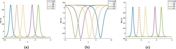
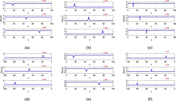
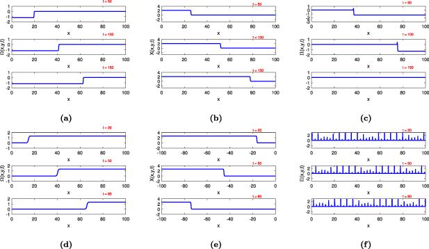
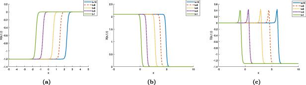
Equation (37) at $t = 1,3,6,8,10$. We display in figure 4(a) that $\Omega(x,1,t)$ is characterized simply by a single soliton profile that maps exactly to the scale of the whole cosine spectrum, without changing the amplitude peak and width, and this offers adequate evidence that although the solution looks sharply singular, it is indeed solitonic. Figure 4(b) consistently propagates $X(x,1,t)$, a bell-shaped positive shape that never changes. Figure 4(c) shows that $\Pi(x,1,t)$ maintains its characteristic positive-amplitude localized structure over the total time order. Physically, the thin but time invariant profile of this solution corresponds well with the behavior of ultra-short pulses in high-energy laser systems, where a strong nonlinearity stifles dispersive broadening even for very steep waveforms. The soliton solutions of equation figure 5 give a tight temporal stability confirmation for equations (35) and (37) at three well separated instances within time. Panels figures 5(a)-(c) are for $\Omega$, $X$ and $\Pi$ in equation (35) at $t = 20,50,80$ and panels figures 5(d)-(f) provide the corresponding fields from equation (37) both at the same time instances. The patterns of the wave profiles are visually identical across the three time snapshots: the amplitude, width, and spatial placement of each feature transition at a constant velocity with no deformation or amplitude decay in any panel. Note that this long-range shape preservation in the stretched time period $t\in[20,80]$ is direct evidence that these solutions are stable traveling waves in the formal sense. To a certain extent, this stability derives from a compromise between the non-linear self-phase modulation conditions and the higher-order dispersive conditions of the AMTZ regime, and it appears to show that these methods can be employed as strong carrier signals in optical fiber networks for long periods of propagation. Figure 6 presents the three-dimensional scale lines and two-dimensional contour maps of the tanh-type soliton solutions obtained from equation (39). Figure 6(a) depicts a kink-antikink primary wave $\Omega(x,y,t)$ which is smooth between two asymptotic values, which physically simulates the propagation of a domain-wall excitation in a ferromagnetic medium or a rarefaction wave in a dispersive plasma. The tanh profile is the canonical solution of the nonlinear-wave equations having competing cubic nonlinearity and linear dispersion, and it can be seen that the AMTZ system has the qualitative nonlinear balance phenomena to exhibit. Figure 6(b) shows the potential field $X(x,y,t)$ propagate as a smooth kink with complementary sign, and expresses the boundary between $X$ and $\Omega$ based on the constraint in equation (8). Figure 6(c) reveals the auxiliary field $\Pi(x,y,t)$ in a sech-squared-shaped shape obtained from tailoring the tanh profile, which is the localized energy density pulse accompanying along the kink. The contour plots 6(d)-(f) show the uniform behavior in the $(x,t)$ plane of all three coupled fields on straight plane paths in figures 6(d)-(f). Figure 7 provides temporal stability validation for equation (39) at $t = 50,100,150$ in panels figures 7(a)-(c), and equation (48) at $t = 20,50,80$ in panels figures 7(d)-(f). For equation (39), the tanh-type kink structure of $\Omega$ is rigidly mapped across the whole domain, and the potential and auxiliary fields all pass at the same rate, which further verified full system coherence on a long temporal domain of $\Delta t = 100$. For equation (48), the compound trigonometric soliton $\Pi$ has a periodic-singular shape at $t = 20,50,80$. The amplitude is indeed strikingly the same. In terms of spatial frequency, even the family members of the trigonometric solution retain their structural identity over large propagation distances. Physically, this robustness indicates that these solutions are not just marginally stable. They lie on the part of completely persistent invariant manifolds of the dynamical system, which makes them ideal candidates for use in dispersive wave transmission. Figure 8 uses colors which depict the time evolution at $t = 1,3,6,8,10$. Figure 8(a) shows the tanh-type dark soliton of $\Omega(x,1,t)$ evenly to the right as a function of time and the transition plateau of the two asymptotic states is perfectly horizontal and with the transition width set. This is the signature of a kink soliton with velocity controlled completely by the wave number parameters $p$, $q$, and $v$ across the propagation coordinate $\xi = px + qy - vt$. Figure 8(b) verifies that the potential $X(x,1,t)$ propagates uniformly, whereas figure 8(c) indicates that the localized sigmoidal shape of $\Pi(x,1,t)$ never abates. The steady rightward drift indicates that the group velocity of the nonlinear wave packet is positive and constant, as can be expected considering the sub-luminal propagation of the dispersive optical media.
Figure 4. The effect of time on the soliton solution of equation (37) at $t = 1,3,6,8,10$: (a) $\Omega(x,1,t)$ exhibiting the singular soliton with sharply peaked amplitude translating without deformation across the spatial domain; (b) $X(x,1,t)$ showing the corresponding potential field evolving uniformly; (c) $\Pi(x,1,t)$ displaying the auxiliary field maintaining its localized singular character through time, confirming solution robustness.
Figure 5. Temporal stability plots of soliton solutions of equations (35) and (37). Each panel shows the wave profile at three time instances $t = 20,50,80$: (a) $\Omega(x,y,t)$ from equation (35) (bright soliton parameters); (b) $X(x,y,t)$ from equation (35); (c) $\Pi(x,y,t)$ from equation (35); (d) $\Omega(x,y,t)$ from equation (37) (singular soliton parameters); (e) $X(x,y,t)$ from equation (37); (f) $\Pi(x,y,t)$ from equation (37). The invariance of the soliton profiles across time confirms wave stability.
Figure 7. Temporal stability plots of the soliton solutions of equations (39) and (48). Panels (a)-(c) show the wave profiles $\Omega$, $X$, $\Pi$ from equation (39) at $t = 50,100,150$; panels (d)-(f) show $\Omega$, $X$, $\Pi$ from equation (48) at $t = 20,50,80$. The invariance of amplitude and shape across all time snapshots confirms the long-range propagation stability of both hyperbolic tangent-type and trigonometric compound-type soliton solutions.
Figure 8. The effect of time on the soliton solution of equation (39) at $t = 1,3,6,8,10$: (a) $\Omega(x,1,t)$ displaying the tanh-type dark soliton profile propagating with constant speed and fixed negative amplitude transition; (b) $X(x,1,t)$ showing the potential function evolving uniformly with time; (c) $\Pi(x,1,t)$ exhibiting the auxiliary wave function maintaining its characteristic sigmoidal shape across all time values, confirming temporal coherence of the traveling wave structure.
Contex soliton solutions presented in equation (48), which involves the combination Figure 9(a) shows that $\Omega(x,y,t)$ is a spatially periodic wave of characteristic asymmetry that comes from the interaction of the tangent component and secant components. With its physical shape, this structure reflects a nonlinear periodic wave train of a class common in plasma lattices and photonic crystal waveguides. As a result of this configuration time is imposed by the medium rather than initial circumstances. Figure 9(b) shows that $X(x,y,t)$ is in fact an osmotically kink type spatial modulation system simultaneously with the oscillatory behavior of $\Omega$, showing clearly the rich multi-component dynamics of an affordable, multi-dimensional AMTZ system. Figure 9(c) depicts $\Pi(x,y,t)$, containing very distinct peaks that directly emerge from a unique $\sec^2$ term at its output, and physically correspond to intense-burst peaks, such as high-intensity burst propagation events in a plasma resonance configuration or multi-photon ion formation in a laser-matter interaction. The contour plots figures 9(d)-(f) also show the regular diagonal propagation of the three fields, and this confirms the regular traveling wave nature of this trigonometric solution family. It displays the time evolution of equation (48) with $t = 1,3,6,8,10$. Figure 10(a) shows that the $\Omega$ component moves uniformly with its asymmetric tan$+$sec profile consistent, indicating that the combined trigonometric nonlinearity supports a stable propagating structure. Figure 10(b) shows that $X(x,1,t)$ has a smooth kink evolution which occurs and the transition location will change at constant speed since this is in agreement with the current velocity of the passing wave. Figure 10(c) shows $\Pi(x,1,t)$ in the form of sharp spikes at points across space, which are always shifted uniformly over time as a function of the poles of $\csc$ and $\sec$ functions, whose coordinates rigidly translate to the current wave. Physically, the periodic singularity structure underlying this solution has the property that the wave phenomena in dissipationless plasmas can be modeled at resonance points at very large amplitudes in the wave field which could have a considerable impact on the mechanism of wave to particle interaction and energy transfer in space plasmas. Figure 11 shows the phase portrait analysis derived from the Galilean transformation (51) for the reduced dynamical system. Figure 11(a) is corresponding to Case 1 ($S_1 \lt 0$, $S_2 \lt 0$), where the equilibrium points $(0,0)$ and $(-1,0)$ are saddle points with real eigenvalues $\lambda_{1,2} = \pm 2$ and $(-\frac{1}{2},0)$ is a center point with purely imaginary eigenvalues $\lambda_{1,2} = \pm\sqrt{-2}$. Phases portrait introduces heteroclinic distances between the pair of saddle points in the center region, with the closed orbits around the center corresponding to periodic wave solutions of AMTZ equation. From a physical point of view, the saddle equilibria correspond to unstable wave propagation modes in which any minor perturbation will cause the trajectory to diverge while the center equilibrium represents stable oscillatory wave packets that move endlessly in phase space without energy loss. Figure 11(b) is Case 2 ($S_1 \gt 0$, $S_2 \gt 0$), and the equilibria configuration is reversed with respect to Case 1: the point $(1,0)$ is a center and has purely imaginary eigenvalues $\lambda_{1,2} = \pm 2$i, and $(\frac{1}{2},0)$ is a saddle with real eigenvalues $\lambda_{1,2} = \pm\sqrt{2}$. Based on this complementary structure, we find that the qualitative dynamics depend on the sign of the product $bv$, which determines the direction the non-linear wave energy concentrates on positive or negative amplitude excitations. Figure 11(c) is Case 3 ($v = 0$) where all equilibrium points coalesce at the origin $(0,0)$ into a cuspidal degenerate equilibrium. This case is related to the static limit of the wave equation where the propagation speed is no longer active, and the phase image becomes cusp-like separatrix. In essence, through the lens of quantum mechanics itself, this critical case represents where qualitatively separated wave propagation regimes cross the threshold for an associated bifurcation of the AMTZ system, that is, from the existence of previously isolated equilibria to a degenerate state at a higher order critical point, and this is what determines how signal propagation systems (nonlinear optical fibers) may undergo a wave amplitude collapse.
Figure 10. The effect of time on the soliton solution of equation (48) at $t = 1,3,6,8,10$: (a) $\Omega(x,1,t)$ showing the tan$+$sec compound trigonometric soliton profile maintaining its asymmetric shape as it propagates rightward; (b) $X(x,1,t)$ exhibiting the potential function with a kink-type transition that shifts consistently with increasing time; (c) $\Pi(x,1,t)$ displaying sharp singular peaks of the auxiliary function at fixed spatial intervals, confirming the periodic singularity structure of this trigonometric-type solution.
Figure 11. The phase portrait of equation (51) for three dynamical cases: (a) Case 1 ($S_1 \lt 0$, $S_2 \lt 0$): two saddle points at $(0,0)$, $(-1,0)$ and one center at $(-\tfrac{1}{2},0)$; (b) Case 2 ($S_1 \gt 0$, $S_2 \gt 0$): two saddle-center pair at $(0,0)$, $(\tfrac{1}{2},0)$, $(1,0)$; (c) Case 3 ($v = 0$): single cuspidal equilibrium at $(0,0)$.
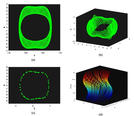
Figure 12 shows the chaotic dynamics of the perturbed system (55) under the parameter set $a = 1$, $b = -0.1$, $\beta = 1$, $p = 1$, $q = 1$, $v = 1$, $\theta = 3$, $\epsilon = 3.6$, for initial condition $(0.91,\,0.99)$. We see the two-dimensional chaotic phase portrait in $(V,\Phi)$ plane with a characteristic attractor with an inscrutable dense, non-repeating trajectory that runs through a bounded region without connecting to a stationary point or a limit cycle figure 12(a). The nonlinear, crossing pattern is a signature of deterministic chaos: the system progresses according to deterministic equations, but its trajectories are exponentially sensitive to the initial state, which makes long-term prediction in practice impossible. Physically, this indicates that the smallest variation on the initial amplitude or phase of the optical pulse will cause quite different wave propagation effects, after sufficient propagation distances, an interesting problem in the design of excellent optical communication systems. Figure 12(b) gives a 3D phase view at $(V,\Phi,W)$ space with $W$ as the time-extended coordinate revealing toroidal geometry of the strange attractor and demonstrating that chaotic dynamics are not a two-dimensional character but rather a real 3D phenomenon with fractal dimension greater than 2. Figure 12(c) is the Poincaré section which resulted through sampling the trajectory over regular phase intervals: non-periodic and scattered distribution of points around the section confirms an absence of regular orbit and geometrically verify their fractal structure. On the other hand, a periodic orbit would only form a finite set of isolated points on the Poincaré section. Figure 12(d) is the three-dimensional Poincaré map with phase-angle colored phases, and we are seeing that the color gradient from blue (low phase) to red (high phase) results in the complex multi-layer structure of the attractor in the extended phase space and confirms that the chaotic motion has a well-defined geometric structure, consistent with a strange attractor, not random noise. Figure 13 has a second chaotic characterization under another parameter regime: $a = 1$, $b = -0.5$, $\beta = 1$, $p = 1$, $q = 1$, $v = 2$, $\theta = -2$, $\epsilon = 0.16$, with a condition of $(0.7,\,0.6)$. Whilst the perturbation amplitude $\epsilon = 0.16$ is much smaller than $\epsilon = 3.6$ of the previous case, the AMTZ system has stable chaotic behavior, indicating that the chaos in this system is not a high-perturbation artifact, but a structurally persistent phenomenon. Figure 13(a) depicts a figure-eight-shaped exotic attractor in $(V,\Phi)$ plane, a geometry that can be physically associated with an unstable equilibrium neighborhood, where a steady state pattern in phase space oscillates between the two unstable neighborhoods in the oscillating wave trajectory, and which corresponds with the homoclinic orbit splitting projected by Melnikov theory near the saddle equilibria described in section 4. Figure 13(b) shows that the three-dimensional size of the attractor is a twisted toroidal structure. The fractal attractor is found to survive the reduced amplitude forcing. Figure 13(c) shows a Poincaré section with widely scattered points, establishing a clear geometric evidence of chaos: the irregular distribution tells us there are no periodic orbit under these forcing conditions. The 3D Poincaré map is illustrated in figure 13(d) with phase coloring, the random arrangement of colored spots in the section confirms that the system is ergodically sampling all the phases, which is a key characteristic of chaotic attractors. Quantitative confirmation that the system is chaotic is provided by Lyapunov exponent analysis and multi-stability plots (figure 14). Figure 14(a) presents time-step transition of two great Lyapunov exponents $\lambda_1$ and $\lambda_2$ in figure 12: after a transient $\lambda_1$ reaches a positive value (approximately $\lambda_1 \approx 0.5 \gt 0$), but $\lambda_2$ shows a negative value implying good quantitative confirmation of chaos. In phase space, the largest Lyapunov exponent in positive direction implies that trajectories near each one of the stations separate exponentially faster with the difference e$ ^{\lambda_1 t}$, and therefore the system is unpredictable to a time of Lyapunov $\tau_L = 1/\lambda_1$. Figure 14(b) depicts the Lyapunov exponents for figure 13 in which, while the forcing amplitude $\epsilon = 0.16$ is smaller, the highest Lyapunov exponent is positive confirming that no matter how small the perturbation, the chaos can be persistent, which is directly relevant to real-world optical systems that always experience small environmental perturbations. Figure 14(c) shows a multi-stability diagram for figure 12, where two trajectories originating from slightly different initial conditions $V(t)$, $\Phi(t)$ gradually diverge into qualitatively different attractors at $t \in [0,200]$, representing visually with a dramatic representation the delicacy of dependence on initial conditions. Figure 14(d) displays multi-stability for figure 13 parameters and the resulting divergence is similar over the time period $t \in [0,300]$, indicating that the intricate basin structure and co-existing attractors are a robust part of the AMTZ system in response to periodic external force. The IMSSEM is much more effective than classic ones including the extended tanh method and the $(G ^{^{\prime}}/G)$ expansion method as it achieves production of all 17 solution families simultaneously from the same algebraic system in this case rather than each function type having to run in a separate manner. All solutions obtained satisfy the original PDE system (1)-(3) and the reduced ODE equation (12) as such, and Maple 2024 back substitution confirmed the zero residuals in every case that was obtained, adding considerable mathematical validation. The comparative table 2 confirms that neither the Myrzakulov-I nor the Myrzakulov-II equation has been investigated via bifurcation or chaos analysis in the existing literature, thus providing the first step in the comprehensive dynamical characterization for the whole family of equations by the Myrzakulov family.
Figure 14. Lyapunov exponent and multi-stability plots confirming chaotic dynamics. (a) Evolution of the two largest Lyapunov exponents $\lambda_1$, $\lambda_2$ over time for the parameter set of figure 12, with the positive largest exponent $\lambda_1 \gt 0$ confirming chaos; (b) Lyapunov exponents for the parameter set of figure 13; (c) Multi-stability plot showing coexisting attractors $V(t)$ and $\Phi(t)$ under the parameters of figure 12; (d) Multi-stability plot for the parameters of figure 13.
Comparative analysis
Table 2 compares the solutions derived in this work against those obtained for related Myrzakulov-type equations in the literature, highlighting the novelty and breadth of the present results.
Physical significance
The analytical solutions obtained in this study have direct physical implications across multiple application domains. The bright soliton solutions equation (37) represent self-focused optical pulses in fiber communications, where the balance between anomalous dispersion and Kerr nonlinearity sustains stable pulse propagation over long distances. The dark soliton solutions correspond to intensity dips in continuous wave backgrounds, relevant to defocusing media and Bose-Einstein condensates. The kink-type solutions model domain wall transitions in ferromagnetic spin chains and topological excitations in plasma. The periodic wave train solutions equations (44)-(50) describe coherent oscillatory structures in mode-locked laser cavities and lattice waves in dispersive plasma. Regarding the dynamical analysis, the coexistence of saddle and center equilibria in phase space directly corresponds to the physical distinction between unstable propagation modes and stable oscillatory wave packets. The positive Lyapunov exponents and fractal Poincaré sections confirm that the AMTZ system, despite being integrable in the unperturbed sense, transitions to chaotic dynamics under external periodic forcing a result of direct relevance to designing perturbation-resistant optical communication links and predicting wave turbulence in plasma.
7. Key findings, limitations, and future directions
Key findings
•
(•)The IMSSEM successfully generated seventeen distinct exact solution families for the AMTZ equation, covering hyperbolic (sech, csch, tanh, coth), trigonometric (tan, cot, sec, csc), and rational function types, representing the most comprehensive analytical treatment of this system to date.
•
(•)Bifurcation analysis revealed three equilibrium configurations saddle, center, and cuspidal points-whose transitions are governed by the sign of the Jacobian determinant $J(V,\Phi)$.
•
(•)Temporal stability analysis confirmed that all soliton solutions preserve their profiles over long propagation distances at time instances $t = 20, 50, 80$ (and $50, 100, 150$), establishing robustness of the solutions.
•
(•)Chaos analysis under external periodic forcing $\epsilon\cos(\theta\xi)$ confirmed strong chaotic dynamics via positive Lyapunov exponents ($\lambda_1 \gt 0$) and fractal Poincaré sections, showing that the integrable system becomes sensitive to initial conditions when perturbed.
Limitations
•
(•)The analytical framework is restricted to traveling wave solutions; non-traveling wave phenomena and lump solutions are beyond the scope of this work.
•
(•)Chaos analysis considered only single-frequency periodic perturbations. Multi-frequency and stochastic disturbances, which are more physically realistic, were not examined.
•
(•)Quantitative stability analysis under continuous parameter variation (e.g. stability regions in parameter space) was not performed.
•
(•)Experimental or numerical validation against physical laboratory settings (optical fiber or plasma experiments) remains to be pursued.
Future directions
•
(•)Extending the solution framework to multi-soliton collisions using the Hirota bilinear method.
•
(•)Deriving rogue wave solutions via Darboux transformations and examining their emergence near saddle-type equilibria.
•
(•)Incorporating fractional-order derivatives to model memory effects in dispersive media.
•
(•)Investigating the $(3+1)$-dimensional generalization of the AMTZ equation and its conservation laws.
•
(•)Designing numerical schemes for non-integrable perturbations and multi-frequency forcing scenarios.
8. Conclusion
This study presented the first comprehensive analytical and dynamical characterization of the AMTZ equation. Using the IMSSEM with the auxiliary ODE $G^{^{\prime} 2} = CG^4 + BG^2 + A$, seventeen families of exact solutions were derived, including hyperbolic (sech, csch, tanh, coth), trigonometric (tan, cot, sec, csc), and rational function types. Bifurcation analysis of the reduced dynamical system identified three equilibrium configurations-saddle, center, and cuspidal points-whose classification is governed by the sign of the Jacobian determinant $J(V,\Phi) = -4b\beta^2p^2q^2a(6V^2p^2 + 6Vbpv + b^2v^2)$. Temporal stability analysis confirmed shape-preserving soliton propagation over long distances. Chaos analysis under external periodic forcing $\epsilon\cos(\theta\xi)$ revealed positive Lyapunov exponents and fractal Poincaré sections, confirming that the integrable AMTZ system exhibits strong sensitivity to perturbations. The key findings, limitations, and future directions are detailed in section 7.
Appendix Verification of solutions via Maple
To verify that the derived solutions satisfy the ODE, we demonstrate the procedure for equation (34) (rational solution). the Maple command odetest(function,ode) returns $0$, confirming exact satisfaction. The Maple code structure is as follows (pseudocode):# Define parametersResult 1 := [a = -B*beta^2*p^2*q^2/(2*b*v^2), b = b, beta = beta, p = p,q = q, v = v, delta[0] = -b*v/(2*p), delta[1] = sqrt(-2*B*C)*v*b/(2*B*p)]# # Define V from Eq.(14)V(xi) = delta[0] + delta[1]*G(xi)# Define G from Eq.(16) G(xi) = 1/(sqrt(C)*(xi + xi__0))# substitute G in V along with Result 1 eq(33)V(xi) = -v*(-sqrt(2)*sqrt(-B*C) + B*sqrt(C)*(xi + xi__0))*b/(2*sqrt(C)*B*p*(xi + xi__0))# Substitute Result 1 into ode Eq.(12)subs(Result 1, ode)-4*beta^2*q^2*B*p^4*V(xi)^3/(b*v^2) - 2*b*beta^2*q^2*B*p^2*V(xi) -p^2*beta^2*q^2*b*diff(diff(V(xi), xi), xi) - 6*beta^2*q^2*B*p^3*V(xi)^2/v = 0;# do substitution function with condition in ode we return zerosubs({A = 0, B = 0}, odetest(V(xi), ode))res := 0
Identical verification was performed for all seventeen solution families, in each case yielding a zero residual upon substitution into the ODE.
WazwazA M2009Partial Differential Equations and Solitary Waves Theory (Nonlinear Physical Science) Springer
2
MahmoodS S, MuradM A S2025Finding optical soliton solutions of the $(4+ 1)$-dimensional Davey-Stewartson-Kadomtsev-Petviashvili equation via multiple techniquesPramana99 151
DemirbilekU, TedjaniA H, SeadawyA R2025Analytical solutions of the combined Kairat-II-X equation: a dynamical perspective on bifurcation, chaos, energy and sensitivityAIMS Math.10 1366413691
MahmoodS S, MuradM A S2025Dynamics of nonlinear wave of the $(3+ 1)$-dimensional Date-Jimbo-Kashiwara-Miwa equation with variable coefficients in inhomogeneous mediaEur. Phys. J. D79 149
KumarS, KumarA2020Dynamical structures of solitons and some new types of exact solutions for the $(2+ 1)$-dimensional DJKM equation using Lie symmetry analysisMod. Phys. Lett. B34 2150015
WangM, XiangzhengLi, ZhangJ2008The ($G^{^{\prime}}/G$)-expansion method and travelling wave solutions of nonlinear evolution equations in mathematical physicsPhys. Lett. A372 417423
MuradM A S, OmarF M, MahmoodS S2025Analyzing the generalized integrable -dimensional nonlinear conformable Schrödinger system via the Kudryashov auxiliary equation method: optical soliton solutionsJ. Opt.54112
MahmoodS S, MuradM A S, RadwanT, AhmedK K, KhalifaA S2026Analysis of time-fractional soliton solutions for Kudryashov's law with dual nonlocal nonlinearity and refractive index in optical fibersAIMS Math.11 23842705
SeadawyA R, Dian-ChenL, ArshadM2018Stability analysis of solitary wave solutions for coupled and $(2+ 1)$-dimensional cubic Klein-Gordon equations and their applicationsCommun. Theor. Phys.69 676
TrikiH, SunY, ZhouQ, BiswasA, YıldırımY, AlshehriH M2022Dark solitary pulses and moving fronts in an optical medium with the higher-order dispersive and nonlinear effectsChaos Solitons Fractals164 112622
DurmusS A, OzdemirN, SecerA, OzisikM, BayramM2024Examination of optical soliton solutions for the perturbed Schrödinger-Hirota equation with anti-cubic law in the presence of spatiotemporal dispersionEur. Phys. J. Plus139 464
RehmanH U, IncM, AsjadM I, HabibA, MunirQ2022New soliton solutions for the space-time fractional modified third order Korteweg-de Vries equationJ. Ocean Eng. Sci.
TariqK U, ZainabH, SeadawyA R, YounisM, RizviS T R, MousaA A A2021On some novel optical wave solutions to the paraxial M-fractional nonlinear Schrödinger dynamical equationOpt. Quantum Electron.53 219
RasoolG, ShafiqA, WangX, ChamkhaA J, WakifA2024Numerical treatment of MHD Al2O3-Cu/engine oil-based nanofluid flow in a Darcy-Forchheimer medium: application of radiative heat and mass transfer lawsInt. J. Mod. Phys. B38 2450129
RezazadehH, KumarD, SulaimanT A, BulutH2019New complex hyperbolic and trigonometric solutions for the generalized conformable fractional Gardner equationMod. Phys. Lett. B33 1950196
RazaN, ArshedS, JavidA2020Optical solitons and stability analysis for the generalized second-order nonlinear Schrödinger equation in an optical fiberInt. J. Nonlinear Sci. Numer. Simul.21 855863
KamelN M, AhmedH M, RabieW B2024Retrieval of soliton solutions for 4th-order $(2+ 1)$-dimensional Schrödinger equation with higher-order odd and even terms by modified Sardar sub-equation methodAin Shams Eng. J.15 102808
OzdemirN, SecerA, BayramM2023Extraction of soliton waves from the longitudinal wave equation with local M-truncated derivativesOpt. Quantum Electron.55 313
BiswasA, EkiciM, SonmezogluA, ZhouQ, MoshokoaS P, BelicM2018Optical soliton perturbation with full nonlinearity for Kundu-Eckhaus equation by extended trial function schemeOptik160 1723
IqbalM, SeadawyA R, DianchenL2019Applications of nonlinear longitudinal wave equation in a magneto-electro-elastic circular rod and new solitary wave solutionsMod. Phys. Lett. B33 1950210
NadeemM, ArqubO A, IamborL F, HussienM, AlzahraniE2025The prospective analysis of three-dimensional time-fractional Helmholtz model using a new iterative methodFractals33 2540069
NadeemM, ArqubO A, AlotaibiF M2025Optical soliton solutions and modulation instability for unstable conformable Schrödinger modelInt. J. Mod. Phys. C36 2450175
BilalM, AlshammariF S, IqbalJ, AhmedK K2026Exploration of the N-soliton solutions for Hodgkin-Huxley model via $ G^{^{\prime}}/G $-expansion methodZ. Angew. Math. Phys.77 68
MustafaM A, MuradM A S2025Soliton solutions to the time-fractional Kudryashov equation: applications of the new direct mapping methodMod. Phys. Lett. B39 2550147
Az-Zo'biE A2019Peakon and solitary wave solutions for the modified Fornberg-Whitham equation using simplest equation methodInt. J. Math. Comput. Sci14 635645
50
Az-Zo'biE A, AfefK, RahmanR U, AkinyemiL, BekirA, AhmadH, TashtoushM A, MahariqI2024Novel topological, non-topological and more solitons of the generalized cubic p-system describing isothermal fluxOpt. Quantum Electron.56 84
TashtoushM A, IbrahimI A, TahaW M, DawiM H, JameelA F, Az-Zo'biE A2024Various closed-form solitonic wave solutions of conformable higher-dimensional Fokas model in fluids and plasma physicsIraqi J. Comput. Sci. Math.5 18
HussainE, ShahS A A, BariqA, ZhaoLi, AhmadM R, RagabA E, Az-Zo'biE A2024Solitonic solutions and stability analysis of Benjamin Bona Mahony Burger equation using two versatile techniquesSci. Rep.14 13520
BiswasF, BiswasS, MondalR I, GoldarS, HassanS S, SardarP2026Chaos and complexity in a novel three-dimensional nonlinear system: analysis, bifurcations and applicationsMath. Methods Appl. Sci.
MathanaranjanT, MyrzakulovR2023Conservation laws, soliton solutions and stability analysis for the Akbota equationResults Phys.54 107086
57
ZahranE H M, AhmadH, RahamanM, IbrahimR A2024Soliton solutions in $(2+ 1)$-dimensional integrable spin systems: an investigation of the Myrzakulov-Lakshmanan equation-IIOpt. Quantum Electron.56 895