

1. Introduction
Every species possesses the ability to perceive environmental sounds. The human ear receives sound waves and vocalizations, transforming them into electrical impulses through the sensory hair cells located within the cochlea. The spiral ganglion neurons transmit the impulses to the brain's hearing center. The loss or damage of hair cells can lead to hearing impairment, which can be managed using a cochlear implant. On the other hand, if the neurons and neural circuitry of the auditory system are injured, the acoustoelectric transformation and the transmission of electrical impulses would be obstructed. The brain's neurons are nurtured and grown in specific areas that serve certain purposes. In particular, efficient photoelectric conversion is used to produce firing patterns in the visual neuron, which is sensitive to optical signals. Auditory neurons [1-3] can detect sound signals when acoustic waves or nonlinear vibrations are transmitted into the auditory system. The auditory pathway is responsible for processing these impulses, which ultimately enables the awareness of sound. Consequently, piezoelectric ceramics could be integrated into the nervous system to transform mechanical vibrations into electrical stimuli, resulting in the creation of a piezoelectric neuron [4-6]. The skin has the capacity to detect small differences in temperature, which in turn could influence the excitability and ion channel activity on the membrane of neuronal cells, ultimately influencing the firing patterns. The output voltage of neural systems could be experimentally linked to temperature sensors. The outcome is the creation of a temperature-dependent neuron [7-10] that could be used to identify potential temperature changes. In addition, the majority of nonlinear systems [11-13] can be made more controllable by the use of periodic external stimuli or variations in the intrinsic characteristics. In this way, patterns resembling those of biological neurons can be induced, including quiescent, bursting, spiking, multiple firing modes, and even chaotic ones.
Information flow between nerve cells is always the foundation of research on hearing impairment correction. A reliable neural model [14, 15] is crucial for assessing and predicting alterations in brain activity patterns, and the effective approach [16] could be used to regulate the collective action of neural systems and synapses [17, 18]. One of the most significant models in neuronal modeling is the FitzHugh-Nagumo (FHN) model [19]. Physical principles state that when energy is pushed via a connected channel, synchronous stability is determined by the energy's balance and propagation [20]. Synchronous neuronal activity is essential for hearing and comprehending auditory information. According to Goossens et al [21], individuals with hearing impairment had asymmetrical right hemisphere synchronization, whereas hearing participants had identical brain synchronization. According to Herrmann et al [22], subclinical hearing impairment could arise from reduced neural activity caused by a lesser sensitivity to sound, even though there is a larger degree of neuronal synchronization in the elderly. Hidalgo et al [23] conducted a controlled experiment in which they compared the hearing normal group to the hearing impaired group. According to their findings, the hearing impaired children exhibited poor performance on all sensorimotor synchronization activities. The hearing-impaired children correctly repeated the number of syllables in the statement for a variety of reasons, including their ability to coordinate complex rhythms. The fundamental process determining temporal coordination is the synchronous rhythm, and the creation of synchronization is connected to several physiological processes [24]. Neuron collaboration via various types of synaptic connections [20, 25, 26] is necessary for the initiation and release of biophysical processes. It also contributes significantly to scientific research, which could change the system's general dynamics in a number of ways [27]. Additionally, a number of studies have shown that weak signals could be processed and amplified by excitable neurons and that chaotic activity could improve the system's sensitivity to weak signals a phenomenon known as chaotic resonance [28]. Chaotic resonance could result from internal chaotic processes or from an external chaotic signal [29].
The intricacy of the brain has led to experiments rather than quantitative theoretical assessments to investigate energy use in the nervous system. There is a connection between the encoding of energy and the metabolism of energy between the mode transition of electrical activity and the development of action potentials in neurons [30]. It could be difficult to accurately identify the energy supply and consumption in neuron and oscillator models, thus the effective energy [31] is utilized to evaluate state-energy dependence using the Helmholtz theorem. The Helmholtz theorem is applied in the FHN model to define a effective energy [32]. This function is employed to describe the energy in certain oscillators. This is a result of the diffuse use of energy during biological systems metabolic processes and the ability of neurons to sustain electrical activity.
The effective energy paradigm goes beyond just being a theoretical idea. It gives us a strong way to analyze how neural systems store information while processing sound. The current theoretical literature suggests that the effective energy is a real energy metric that controls the underlying neuronal manifold. This formulation is essential for elucidating systemic stability. In particular, it explains how neural circuits stay very sensitive to changes in membrane potential. This lets the system respond almost instantly to outside stimuli while also making sure that there is a controlled restorative phase to stop excitotoxicity. Recent developments in quasi effective energy neural dynamics show that these mathematical models can accurately simulate the complicated spiking and bursting patterns seen in real neuronal populations. These models effectively encapsulate such behaviors, thereby associating physical energy concepts with observed neural activity [33, 34].
Maintaining stable energy topography is very important for the auditory system to work properly. This energy landscape is the base for the precise rhythmic firing patterns that are needed for accurate sound encoding. However, evidence shows that the way this landscape is set up makes it very vulnerable to damage from aging and long-term exposure to noise. Tests of auditory nerve function show that these stressors greatly reduce the intensity and temporal precision of neural responses, especially in environments with a lot of noise [35].
The resulting impairment encompasses more than mere signal loss. It breaks up sound sequences and messes with the brain's ability to keep signals coherent. When the underlying architecture fails to convert acoustic stimuli into coherent representations, a functional disconnection from the auditory environment ensues. This failure shows how important it is to have an analytical framework based on effective energy. The study can effectively map the shift between functional synchronization and pathological instability by using energy landscape models that interpret neural activity as transitions between different energy states. These kinds of models help us understand the exact energy levels that cause sensory loss and give us a plan for possible adaptive interventions that could help improve hearing health.
The current study employs dynamic stimuli defined by spectral evolution to assess the correlation between neural energy states and electrical responses. We examine the effective energy intrinsic to the system by utilizing time-dependent external stimulation based on the decomposition principles of Helmholtz's theorem. This methodological framework facilitates the accurate observation of energy fluctuations and the consequent modulation of neuronal activity. The results show that random background noise and chaotic sounds have a big effect on how neurons behave. Stable environmental conditions help neurons work together, but chaotic landscapes create complex noise-driven dynamics that either boost or lower certain neural responses. These findings clarify the nonlinear interactions between auditory signals and noisy environments, while also establishing a strong link between sound input, energy dynamics, and neural synchronization. In the end, this model gives us a mechanistic physical understanding of how complex neural networks self-organize, spike, and burst.
The structure of the paper is outlined as follows: in section 2 , we develop and describe the mathematical framework that forms our investigation. Section 3 introduces the effective energy function, followed by an in-depth analysis of the system's dynamic behavior. This includes a thorough discussion of the observed phenomena, along with corresponding visualizations of the simulation results to illustrate key patterns and trends. Lastly, in section 4 , we provide concluding remarks, highlighting the study's main contributions and suggesting potential directions for future research.
2. Proposed model
In the biological system, the processing of auditory information comprises the receipt of sound, the conversion of acoustoelectric energy, and the transmission of the neural pulse to the nerve center. The ear is responsible for receiving sound, which in turn causes the tympanic membrane along with various structures to vibrate. The vibration is then communicated to spiral tissue that is found in the cochlea, which is composed of hair cells and supporting cells. In addition to being sensitive to sound waves, each hair cell contacts vestibular nerves in order to facilitate the development of synaptic connections. The cilia are attached to the tectorial membrane that envelops the hair cells. To activate the tectorial membrane, the lymphoid fluid could go through the external sonic wave. The hair cells are then forced to produce a nerve pulse, which stimulates the spiral ganglion neurons. The auditory center then records the proper action potential that is produced.
In neuronal models, a time-dependent external current of the form $ I_\mathrm{ext} = I\cos(2\pi\omega t) $ is, in general, interpreted as an externally imposed electrical forcing. Such a term by itself does not imply any specific physical origin and therefore cannot automatically be regarded as a piezoelectric current. The mathematical form of a sinusoidal function alone is insufficient to characterize the underlying physical mechanism.
However, this same expression can be legitimately interpreted as a piezoelectric ceramic current if its origin is explicitly linked to electromechanical transduction. In particular, when a piezoelectric ceramic is incorporated into a neural circuit, external mechanical stimulation such as acoustic pressure or vibration induces mechanical deformation in the material. Owing to the piezoelectric effect, this deformation generates electric charge according to the constitutive relation $Q = d_{33}F$, where d33 is the piezoelectric coefficient and F denotes the applied mechanical force. The time variation of this charge produces an electric current, which acts as an effective stimulus to the neural circuit.
Assuming that the external mechanical excitation is harmonic, i.e. $F(t) = F_0\cos(2\pi\omega t)$, then the resulting electrical response of the piezoelectric ceramic is also periodic. Under the linear piezoelectric approximation and neglecting higher-order mechanical dynamics, the effective electrical output of the ceramic can be modeled phenomenologically as $I_\mathrm{pz}(t) = I\cos(2\pi\omega t)$, where the amplitude I implicitly depends on the piezoelectric parameters, material geometry, and the intensity of the mechanical excitation.
Accordingly, when the external current term in the neuron model is defined as $\xi U_\mathrm{PC} = I_\mathrm{ext}(t) = I\cos(2\pi\omega t)$, and $U_\mathrm{PC} $ is explicitly identified as the electrical output generated by a piezoelectric ceramic driven by mechanical stimulation, the term $I_\mathrm{ext}$ can be consistently interpreted as a piezoelectric ceramic current. In this context, the sinusoidal current is not an arbitrarily imposed electrical input but rather the electrical manifestation of acoustic-to-electric energy conversion mediated by the piezoelectric element.
A memristor is characterized by a constitutive relationship between the electric charge q and the magnetic flux $\phi$, originally introduced by Chua [36] as the fourth fundamental passive element. In a flux-controlled formulation, the memristive behavior is described by a nonlinear charge-flux relation $q = q(\phi)$, and the associated memductance is defined as $M(\phi) = \mathrm{d}q(\phi)/\mathrm{d}\phi$, which determines the state-dependent coupling between voltage and current. Following commonly adopted modeling approaches in the literature, a smooth monotone-increasing cubic nonlinearity is assumed in the form
$q(\phi)=\alpha \phi+\beta \phi^{3}, \quad \alpha, \beta>0,$
from which the memductance is obtained as $M(\phi) = \alpha+3\beta\phi^{2}$. This formulation captures the essential memory-dependent and nonlinear characteristics of memristive behavior and has been widely employed in the study of nonlinear dynamical systems and neuron models to represent electromagnetic induction effects and history-dependent feedback mechanisms.Piezoelectric ceramics were used in order to transform an external sound wave into an electric stimulus. This was accomplished via the creation of a similar artificial signal processor. For the purpose of triggering unique dynamic behaviors, this technique makes it easier to generate a variety of firing patterns inside the neuronal circuit. Consequently, the neuronal networks will be activated, which will result in an increase in the general sensitivity of the system to inputs from the outside world. The biological and physical processes that underlie the operation of the auditory system served as the inspiration for this technique. This approach improves the realism of neural response modeling by drawing on ideas from the field of auditory processing. Together with a piezoelectric ceramic element and an operational brain system that is sensitive to external sonic waves, we have replaced the source and the external stimulus in order to simplify the procedure. It is the intention of this replacement to make the interaction between the brain system and the auditory impulses that are applied easier to do successfully. The electromagnetic induction current is caused by a potential difference that exists between two neurons. Numerous recent studies have highlighted the substantial impact of magnetic flux coupling [37-40] on the dynamic properties of neuronal activity. This study explores how magnetic flux influences the dynamic behavior of the coupled FHN model. The dynamic equations of the enhanced FHN neuron model, influenced by the external stimulation current, are identified as follows, as shown in figure 1:
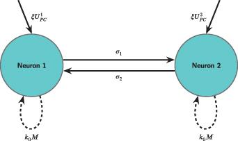
Figure 1. Schematic representation of a two FHN neuronal network with memristive autapses and synaptic coupling. |
$\begin{align} \begin{split} \frac{\mathrm{d}v_{1}}{\mathrm{d}t} &= v_1\left(1-\xi\right) - a_1 v_{1}^3 -u_1+\xi U_{PC}^{1} \\ &\quad + k_{0} M\left(\phi\right)v_{1} + \sigma_{1}\left(v_{2}-v_{1}\right),\\ \frac{\mathrm{d}u_{1}}{\mathrm{d}t} &= c\left( v_1 + a-b u_1\right),\\ \frac{\mathrm{d}v_{2}}{\mathrm{d}t} &= v_2\left(1-\xi\right) - a_1 v_{2}^3 -u_2+\xi U_{PC}^{2} \\ &\quad + k_{0} M\left(\phi\right)v_{2} + \sigma_{2}\left(v_{1}-v_{2}\right),\\ \frac{\mathrm{d}u_{2}}{\mathrm{d}t} &= c\left( v_2 + a-b u_2\right),\\ \frac{\mathrm{d}\phi}{\mathrm{d}t } &= k_{1}\left(v_1 -v_2\right) - k_{2} \phi, \end{split}\end{align}$
in which, $\begin{align} M\left(\phi\right) = \alpha + 3 \beta \phi^2.\end{align}$
The variables u1 and u2 denote the state components corresponding to ion exchange dynamics across the membranes of two neurons, while v1 and v2 represent the membrane potentials of these adjacent neurons. The feedback current term, $k_0M(\phi)v_{j}, j = 1,2$, models the influence of membrane potential induced by electromagnetic feedback, where k0 signifies the feedback gain coefficient. For the purposes of numerical simulation and analysis, the model was evaluated using the following set of parameter values: $\begin{align} \begin{split} & a = 0.7;\;b = 0.6;\;\xi = 0.1;\;a_1 = 1/3;\\ & c = 0.1;\;k_{0} = 0.1;\;k_{1} = 0.8;\;k_{2} = 0.2;\\ & \sigma_{1} = 1.2;\;\sigma_{2} = 0.5;\;\alpha = 0.1;\;\beta = 0.2 \,. \end{split}\end{align}$
The memristive term in equation (According to the Faraday law of electromagnetic induction, the term $k_0M(\phi)v_{j}, j \in \{1,2\}$ is derived from 'equation (2 )', and it is stated as follows:
$\begin{align} i = \frac{\mathrm{d}q\left(\phi\right)}{\mathrm{d}t} = \frac{\mathrm{d}q\left(\phi\right)}{\mathrm{d} \phi}\frac{\mathrm{d}\phi}{\mathrm{d}t} = M\left(\phi\right)V = k_0 M\left(\phi\right)v.\end{align}$
Here, V represents the electromotive force, which drives the electrical activity of the system, while k0 denotes the feedback gain parameter that regulates the strength of the response through the feedback mechanism [41].The piezoelectric input is modeled as a harmonic driving term,
$\xi U_{p c}^{(j)}=I_{j} \cos (2 \pi \omega t), \quad j=1,2 .$
This choice is motivated by the fact that acoustic pressure waves are naturally oscillatory, and piezoelectric materials respond almost linearly when subjected to small deformations. Here, Ij is taken as the driving amplitude applied to the jth neuron and represents how strongly the acoustic signal is transferred to the neuron through the piezoelectric element. From a biological point of view, this periodic input reflects the regular mechanical vibrations experienced in the auditory system, where neurons respond to repeated membrane motion that follows the sound frequency. With this representation, sensory-driven neural excitation can be described in a straightforward way that remains physically and biologically meaningful, while allowing resonance and synchronization effects to be examined.3. Results and discussion
3.1. Effective energy function of the coupled FHN neurons
Information transfer and the encoding of energy are fundamental to the signal processing mechanisms underlying neuronal electrical activity [42]. The absorption and emission of electromagnetic energy are intimately connected to the biological discharge process of neurons inside the neural network [43]. The vector field is assumed to be continuously differentiable and bounded on a simply connected domain $\Omega \in \mathbb{R}^5$ in the state space. According to the Helmholtz theorem, each vector field in space could be separated in to a gradient and vortex field superposition. A gradient plus a curl could be used to define the generic vector function of position, as seen below, and the Helmholtz theorem [44] can be used to calculate effective energy, 2 ) can be reformulated in the following manner:
$\begin{align} F\left(\boldsymbol{r},t\right) = F_{c}\left(\boldsymbol{r}\right) +F_{d}\left(\boldsymbol{r}\right) + F_{e}\left(\boldsymbol{r},t\right).\end{align}$
Hence, the dynamical system described by equation ($\begin{align} \begin{pmatrix} \dot v_{1} \\ \dot u_{1}\\ \dot v_{2} \\ \dot u_{2} \\ \dot \phi \end{pmatrix} & = F_{c}\left(v_1,u_1,v_2,u_2,\phi\right) +F_{d}\left(v_1,u_1,v_2,u_2,\phi\right) \nonumber\\ &\quad + F_{e}\left(v_1,u_1,v_2,u_2,\phi,t\right).\end{align}$
In equation (8 ), the conservative along with dissipative components are represented by the terms $F_{c}(v_1,u_1,v_2,u_2,\phi)$ and $F_{d}(v_1,u_1,v_2,u_2,\phi)$ respectively. The gradient matrix of the effective energy function $H(v_1,u_1,v_2,u_2,\phi)$ is represented by the symbol $\nabla H$. The effective energy function H and the change of energy results from the work done in the force field, H could be defined as follows: 8 ) and (9 ) and is expressed as follows: 13 ) constitutes a first-order linear homogeneous partial differential equation for the effective energy function H. The coefficient vector field appearing in this equation is continuously differentiable over the considered state-space domain. It is well established that such equations admit solutions in the form of first integrals of the associated characteristic system. Accordingly, the effective energy function given in equation (14 ) is obtained by integrating the characteristic equations corresponding to equation (13 ), which ensures the internal consistency of the effective energy formulation. The general solution, as derived from equation (13 ), can be written as:
$\begin{align} \begin{cases} \nabla H^{\mathrm{T}}F_{c}\left(v_1,u_1,v_2,u_2,\phi\right) = 0,\\ \frac{\mathrm{d}H}{\mathrm{d}t} = \nabla H^{\mathrm{T}}\left( F_{d}\left(v_1,u_1,v_2,u_2,\phi\right) + F_{e}\left(v_1,u_1,v_2,u_2,\phi,t\right)\right). \end{cases}\end{align}$
The system's dynamics can be decomposed into dissipative and conservative parts, which are respectively expressed as: $align$
$\begin{align} & F_{d}\left(v_1,u_1,v_2,u_2,\phi\right)\nonumber\\ & \quad = \begin{pmatrix} v_1\left(1-\xi\right) -a_1v_{1}^3 + k_0 M\left(\phi\right)v_1 - \sigma_1v_1 + \phi\\ -cbu_1\\ v_2\left(1-\xi\right) -a_1v_{2}^3 + k_0 M\left(\phi\right)v_2 - \sigma_2v_2 + \frac{\sigma_2}{\sigma_1}\phi\\ -cbu_2\\ -k_2 \phi \end{pmatrix},\end{align}$
$align$
The effective energy function $H(v_1,u_1,v_2,u_2,\phi)$, describing the coupled neuron dynamics, can be derived from equations ($\begin{align} &\left(-u_1 +\sigma_1 v_2 -\phi\right)\frac{\partial H}{\partial v_1} + c\left(v_1 + a\right)\frac{\partial H}{\partial u_1} \nonumber\\ &\quad+ \left(-u_2 +\sigma_2 v_1 -\frac{\sigma_2}{\sigma_1}\phi\right)\frac{\partial H}{\partial v_2} + c\left(v_2 + a\right)\frac{\partial H}{\partial u_2} \nonumber\\ &\quad + k_1\left( v_1 -v_2\right) \frac{\partial H}{\partial \phi} = 0.\end{align}$
Equation ($\begin{align} H & = \left(-u_1 + \sigma_1 v_2 -\phi\right)^2 +c\left(v_{1}^2+2av_1\right)\nonumber\\ &\quad - \frac{\sigma_1}{\sigma_2}\left(-u_2 +\sigma_2 v_1 -\frac{\sigma_2}{\sigma_1}\phi\right)^2\nonumber\\ &\quad - c\frac{\sigma_1}{\sigma_2}\left(v_2^2 +2av_2 \right) + k_1 \left(v_1-v_2\right)^2.\end{align}$
The rate of change in the effective energy function over time is given by $\begin{align} \frac{\mathrm{d}H}{\mathrm{d}t} & = 2(-u_1 + \sigma_1 v_2 -\phi)(-\dot u_1 + \sigma_1 \dot v_2 -\dot \phi) \nonumber\\ &\quad- 2\frac{\sigma_1}{\sigma_2}(-u_2 +\sigma_2 v_1 -\frac{\sigma_2}{\sigma_1}\phi)(-\dot u_2 +\sigma_2 \dot v_1 -\frac{\sigma_2}{\sigma_1} \dot \phi) \nonumber\\ &\quad +c(2v_{1} \dot v_1+2a \dot v_1) -c \frac{\sigma_1}{\sigma_2}(2v_2 \dot v_2 +2a \dot v_2 )\nonumber\\ &\quad + 2k_1 (v_1-v_2)(\dot v_1 - \dot v_2)\nonumber\\ & = \Bigl(2c(v_1+a)-2\sigma_1(-u_2+\sigma_2v_1-\frac{\sigma_2}{\sigma_1}\phi) + 2k_1(v_1-v_2)\Bigl)\nonumber\\ &\quad \times \dot v_1 -2 (-u_1+\sigma_1v_2-\phi)\dot u_1 \nonumber\\ &\quad + \Bigl( -2c\frac{\sigma_1}{\sigma_2}(v_2+a)+2\sigma_1(-u_1+\sigma_1v_2-\phi) \nonumber\\ &\quad-2k_1(v_1-v_2) \Bigl) \dot v_2 +2\frac{\sigma_1}{\sigma_2}(-u_2+\sigma_2v_1 - \frac{\sigma_2}{\sigma_1}\phi)\dot u_2 \nonumber\\ &\quad +\Bigl(-2(-u_1+\sigma_1v_2-\phi) + 2(-u_2+\sigma_2v_1-\frac{\sigma_2}{\sigma_1}\phi)\Bigl) \dot \phi\,. \end{align}$
With slightly algebraic manipulation, it is easy to demonstrate that $\begin{align} \frac{\mathrm{d}H}{\mathrm{d}t} & = \Bigl(2c(v_1+a)-2\sigma_1(-u_2+\sigma_2v_1-\frac{\sigma_2}{\sigma_1}\phi) + 2k_1(v_1-v_2)\Bigl)\nonumber\\ &\quad\times \Bigl( v_1(1-\xi) -a_1v_{1}^3 + k_0 M(\phi)v_1 \nonumber\\ &\quad - \sigma_1v_1 + \phi + I_1 \cos(2\pi\omega t)\Bigl) +2 (-u_1+\sigma_1v_2-\phi)(cbu_1) \nonumber\\ &\quad + \Bigl(- 2c\frac{\sigma_1}{\sigma_2}(v_2+a)+2\sigma_1(-u_1+\sigma_1v_2-\phi) \nonumber\\ &\quad-2k_1(v_1-v_2) \Bigl) \Bigl(v_2(1-\xi) -a_1v_{2}^3 + k_0 M(\phi)v_2 \nonumber\\ &\quad- \sigma_2v_2 - \frac{\sigma_2}{\sigma_1}\phi +I_2\cos(2\pi\omega t)\Bigl) \nonumber\\ &\quad+2\frac{\sigma_1}{\sigma_2}(-u_2+\sigma_2v_1 - \frac{\sigma_2}{\sigma_1}\phi)(-cbu_2) \nonumber\\ &\quad +\Bigl(-2(-u_1+\sigma_1v_2-\phi) + 2(-u_2+\sigma_2v_1-\frac{\sigma_2}{\sigma_1}\phi)\Bigl) \nonumber\\ &\quad\times (-k_2 \phi). \end{align}$
Furthermore,$\begin{align} & \nabla H^{\mathrm{T}} \left(F_{d}+F_e\right) = \left(\frac{\partial H}{\partial v_1} \frac{\partial H}{\partial u_1} \frac{\partial H}{\partial v_2} \frac{\partial H}{\partial u_2} \frac{\partial H}{\partial \phi} \right)\nonumber\\ &\,\,\,\,\,\times \begin{pmatrix} v_1\left(1-\xi\right) -a_1v_{1}^3 + k_0 M\left(\phi\right)v_1 - \sigma_1v_1 + \phi +I_1 \cos\left(2 \pi\omega t\right)\\ -cbu_1\\ v_2\left(1-\xi\right) -a_1v_{2}^3 + k_0 M\left(\phi\right)v_2 - \sigma_2v_2 + \frac{\sigma_2}{\sigma_1}\phi + I_2 \cos\left(2 \pi \omega t\right)\\ -cbu_2\\ -k_2 \phi \end{pmatrix}, \end{align}$
along with, $\begin{align} \frac{\partial H}{\partial v_1} & = 2\left( c\left(v_1+a\right)-\sigma_1\left(-u_2+\sigma_2v_1-\frac{\sigma_2}{\sigma_1}\phi\right) + k_1\left(v_1-v_2\right)\right),\nonumber\\ \frac{\partial H}{\partial u_1} & = -2\left(-u_1+\sigma_1v_2-\phi \right),\nonumber\\ \frac{\partial H}{\partial v_2}& = 2\left(-c\frac{\sigma_1}{\sigma_2}\left(v_2+a\right)+\sigma_1\left(-u_1+\sigma_1v_2-\phi\right) -k_1\left(v_1-v_2\right)\right), \nonumber\\ \frac{\partial H}{\partial u_2} & = 2\frac{\sigma_1}{\sigma_2}\left(-u_2+\sigma_2v_1 - \frac{\sigma_2}{\sigma_1}\phi\right),\nonumber\\ \frac{\partial H}{\partial \phi} &= -2\left(-u_1+\sigma_1v_2-\phi\right) + 2\left(-u_2+\sigma_2v_1-\frac{\sigma_2}{\sigma_1}\phi\right). \end{align}$
Hence, $\begin{align} &\nabla H^{\mathrm{T}} \Bigl(F_{d}+F_e\Bigl) \nonumber\\ &\quad= \Bigl(2c(v_1+a)-2\sigma_1(-u_2+\sigma_2v_1-\frac{\sigma_2}{\sigma_1}\phi) + 2k_1(v_1-v_2)\Bigl)\nonumber\\ &\quad\times \Bigl( v_1(1-\xi) -a_1v_{1}^3 + k_0 M(\phi)v_1 - \sigma_1v_1 \nonumber\\ &\quad + \phi + I_1 \cos(2\pi\omega t)\Bigl) +2 (-u_1+\sigma_1v_2-\phi)(cbu_1)\nonumber \\ &\quad + \Bigl( -2c\frac{\sigma_1}{\sigma_2}(v_2+a)+2\sigma_1(-u_1+\sigma_1v_2-\phi) -2k_1(v_1-v_2) \Bigl)\nonumber\\ &\quad\times \Bigl(v_2(1-\xi) -a_1v_{2}^3 + k_0 M(\phi)v_2 - \sigma_2v_2 \nonumber\\ &\quad + \frac{\sigma_2}{\sigma_1}\phi +I_2\cos(2\pi\omega t)\Bigl) +2\frac{\sigma_1}{\sigma_2}(-u_2+\sigma_2v_1 - \frac{\sigma_2}{\sigma_1}\phi)(-cbu_2) \nonumber\\ &\quad +\Bigl(-2(-u_1+\sigma_1v_2-\phi) + 2(-u_2+\sigma_2v_1-\frac{\sigma_2}{\sigma_1}\phi)\Bigl) (-k_2 \phi). \end{align}$
By combining equations (In this work, we use average energy to describe a neuron's activity over time. Looking only at instantaneous energy is not very helpful, because it changes quickly and irregularly. By averaging the energy, we obtain a quantity that reflects the system's typical behavior over a more extended period. This average is computed from a effective energy-type expression that includes the neuron's own dynamics, the applied input, and interactions within the network. This measure makes it easier to distinguish different patterns of neural activity, such as resting states, regular firing, bursting, and irregular oscillations. Changes in the average energy reflect how the system reacts when inputs or parameters are modified, and whether neurons tend to act together or independently. Overall, the average energy helps indicate whether the system remains stable and how it responds to changing conditions. To evaluate the sustained energetic dynamics of the neuron, the average energy $\lt{H}\gt$ is computed by integrating the energy function H over a complete time interval T1,
$\begin{align} \lt H \gt = \frac{1}{T_1} \int_{0}^{T_1} H\mathrm{d}t.\end{align}$
3.2. Numerical simulation
During the process of converting an external auditory wave into a comparable electrical stimulus, the cell membrane is responsible for capturing and recording the energy that is presented from the outside. Electric stimulation causes the membrane of a neuron to become polarized and magnetized, and it also causes the excitability of the neuron to change, which in turn causes the firing patterns of brain activity to develop differently. By introducing periodic forcing into the external stimulation current inside the model (2 ), this part investigates the electrical activity of the neuron as well as the effective energy of the organism. This periodic component will be introduced in order to explore the impact that it has on the dynamic response and energy profile of the neuron.
Figure 2 shows that when the angular frequency is properly managed, the firing pattern could be controlled to display bursting, spiking, periodic firing, and, finally, chaotic modes. In the case where the angular frequency is held constant, the correct selection of the amplitude of the auditory wave could also be an efficient method for regulating the firing types of brain processes.

Figure 2. Firing patterns of the neuron under different input frequencies: (a) bursting behavior at low frequency $\omega$ = 0.005, (b) spiking at moderate frequency $\omega$ = 0.015, (c) periodic behavior at higher frequency $\omega$ = 0.05, and (d) chaotic firing at high frequency $\omega$ = 0.15. Each subplot illustrates the membrane potential dynamics for a specific external stimulation frequency, demonstrating the transition across distinct firing regimes when $I_1 = 0.6 ~\&~ I_2 = 0.6$. |
3.2.1. The impact of various factors on electrical activity and effective energy.
The expanded FHN model should account for the different elements since the external mixed current variety could also alter the model of the neural electrical activity, which could alter the effective energy. In order to determine the effective energy and its derivative, an analysis will be carried out under the conditions of variable amplitude I1 and I2 of the periodic impressed source. The system enters an autonomous state when I1 and I2 is equal to zero. When the system (2 ), which has a starting state value of $(0.1, 0.2, 0.1, 0.2, 0.1)$, is considered, the value of H(0) is equal to 0.027. System (2 ) phase diagram is shown in figures 3(e)-(h), and figures 3(a) and (b) shows the state variable v1 and v2 against time. In addition, the development of the effective energy and its derivative across time is seen in figure 3(c) and (d), respectively. According to these illustrations, $ \frac{\mathrm{d}H}{\mathrm{d}t}$ is non-zero for the first time interval and then settles at 0, causing the effective energy H to fluctuate up, down, and then settle at a constant value. Furthermore, it is possible to interpret the remaining electrical energy in the system (2 ) after fluctuations as being preserved inside the memristor, demonstrating its non-volatile nature. The memristor's ability to save energy steadily is validated by the last stable point, when $v_1 ~\&~ v_2$ achieve values of -1.0426, showing a linear connection with the state variable $\phi$. To evaluate the sustained energetic dynamics of the neuron, the average energy $\lt{H}\gt $ is computed by integrating the energy function H over a complete time interval T1 = 1000, yielding an average value of approximately $\lt{H}\gt = 0.465~97.$ The resting state depicted in figure 3 represents a stable dynamical regime in which the system asymptotically converges to an equilibrium or a stable low-amplitude response, without exhibiting sustained oscillations. This behavior proffers that, given the parameter values corresponding to it, dissipative processes comprise the majority of the system dynamics, which in turn prevents the onset of oscillatory behavior. The inclusion of the resting state is significant, as it provides a baseline reference for the system's dynamical behavior and facilitates a clear comparison with oscillatory and complex regimes. Moreover, it helps to illustrate the parameter-dependent transition from inactive states to active dynamical behaviors as system parameters are varied.
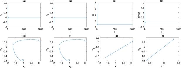
Figure 3. Dynamical evolution of the energy function and action potential under external stimulation. Subfigures (a) and (b) show the state variables v1 and v2, (c) shows the effective energy H, and (d) its time derivative $\frac{\mathrm{d}H}{\mathrm{d}t}$. Phase-space trajectories are presented in (e)-(h). Simulations are performed for external currents $I_1 = 0.0$ and $I_2 = 0.0$, illustrating how the stimuli influence both the energy dynamics and neuronal firing behavior. |
The state variable v1 and v2 over time and the phase diagram for the system (2 ), which starts with an initial state value of $(0.1, 0.2, 0.1, 0.2, 0.1)$, and I1 and $ I_2 = 0.6$ are shown in figures 4(a) and (b) as well as (e)-(h) respectively. In addition, the evolution of effective energy H and its derivative $\frac{\mathrm{d}H}{\mathrm{d}t}$ with time are shown in figures 4(c) and (d), respectively. These illustrations show that throughout time, $\frac{\mathrm{d}H}{\mathrm{d}t}$ swings frequently about 0, which causes the system to oscillate repeatedly and inject and consume effective energy H of the systems (2 ). This behavior arises from the non-conservative nature of the system, in which the active memristive element injects energy in a state-dependent manner, whereas the resistive component continuously dissipates energy. During each oscillation period, these two effects act alternately and balance each other on average, resulting in zero net energy variation over one cycle. Therefore, the effective energy analysis suggests that the self-sustained periodic oscillation has a physical cause that can be described as a dynamic equilibrium between the injection of energy and its elimination. Standard dynamical indicators, such as phase portraits or state trajectories, are insufficient to infer this energy process when used in isolation. There is an estimated value of 1.5157 for the calculated average energy $\lt{H}\gt $ for the time period T1. Through a dynamic equilibrium between energy injection from the active memristive element and energy dissipation generated by resistive effects, this illustrates that the oscillatory state is maintained at a well-defined energetic level. This is accomplished via dynamic balancing.
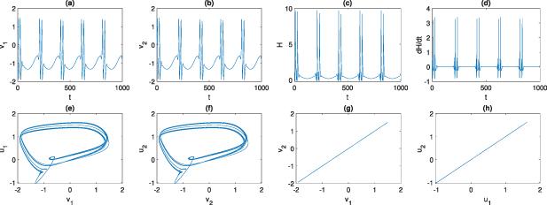
Figure 4. Dynamical evolution of the energy function and action potential under external stimulation. Subfigures (a) and (b) show the state variables v1 and v2, (c) shows the effective energy H, and (d) its time derivative $\frac{\mathrm{d}H}{\mathrm{d}t}$. Phase-space trajectories are presented in (e)-(h). Simulations are performed for external currents $I_1 = 0.6$ and $I_2 = 0.6$, illustrating how the stimuli influence both the energy dynamics and neuronal firing behavior. |
The time evolution of the state variables v1 and v2, along with the phase diagram of the system (2 ), are illustrated in figure 5. The system begins with an initial state of $ (0.1, 0.2, 0.1, 0.2, 0.1) $, with input currents $ I_1 = 1.2 $ and $ I_2 = 0.8 $. Figures 5(a) and (b) depict the state variable dynamics, while figures 5(e)-(h) present the corresponding phase diagrams. The dynamic behavior appears to be characterized by chaotic oscillations within the system. Furthermore, we can see in figure 5(c) and (d) how effective energy H and its derivative $\frac{\mathrm{d}H}{\mathrm{d}t}$ change with time. The diagram visually represents these changes and highlights the evolution of the system's dynamic behavior. Over time, $\frac{\mathrm{d}H}{\mathrm{d}t}$ shows chaotic variations about 0, which causes the effective energy H to oscillate chaotically. Chaotic oscillations are produced as a result of the chaotic intertwined genesis of energy input and consumption. The computed average energy $\lt{H}\gt $ over the time period T1 is approximately 1.8672. The bursting dynamics arise from fast-slow interactions within the system, where the effective energy describes the alternating accumulation and release of energy that drives transitions between silent and active spiking phases.
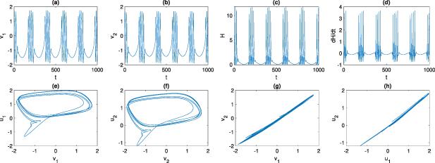
Figure 5. Dynamical evolution of the energy function and action potential under external stimulation. Subfigures (a) and (b) show the state variables v1 and v2, (c) shows the effective energy H, and (d) its time derivative $\frac{\mathrm{d}H}{\mathrm{d}t}$. Phase-space trajectories are presented in (e)-(h). Simulations are performed for external currents $I_1 = 1.2$ and $I_2 = 0.8$, illustrating how the stimuli influence both the energy dynamics and neuronal firing behavior. |
Figure 6 presents the time evolution of the state variables v1 and v2 along with the phase diagram of the system (2 ). The system begins with an initial state of $(0.1, 0.2, 0.1, 0.2, 0.1)$ and operates under input currents $I_1 = 1.8$ and $I_2 = 1.2$. The state variable trajectories are shown in figures 6(a) and (b), while figures 6(e)-(h) illustrate the corresponding phase space representations. The dynamic behavior is reflected in the presence of bursting oscillations. In result, piezoelectric ceramics have the potential to be integrated into the brain system, which would allow for the collection and encoding of external auditory waves. The computed average energy $\lt{H}\gt $ over the time period T1 is approximately 2.3688. Stronger bursting strengthens the fast-slow internal dynamics and amplifies oscillations in the effective energy, indicating increased energy accumulation and release.
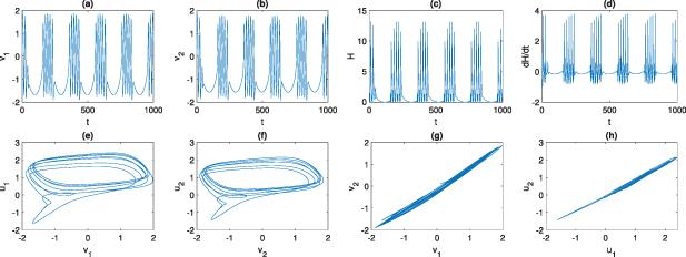
Figure 6. Dynamical evolution of the energy function and action potential under external stimulation. Subfigures (a) and (b) show the state variables v1 and v2, (c) shows the effective energy H, and (d) its time derivative $\frac{\mathrm{d}H}{\mathrm{d}t}$. Phase-space trajectories are presented in (e)-(h). Simulations are performed for external currents $I_1 = 1.8$ and $I_2 = 1.2$, illustrating how the stimuli influence both the energy dynamics and neuronal firing behavior. |
We investigated the types of neuronal firing activities that arise during transitions between different electrical states by computing the Lyapunov exponent curves. The diagrams show that the dynamics of the two-neuron network progress from periodic to quasiperiodic behavior and exhibit several phases of chaotic firing activity. Figure 7 presents the variation of the largest Lyapunov exponent (LLE) with respect to three principal control parameters: figure 7(a) parameter $\omega$, figure 7(b) the external current I1, and figure 7(c) the external current I2. In figure 7(a), modulation of $\omega$ demonstrates a transition from regimes with negative LLE values, corresponding to stable resting states or periodic spiking, to intervals where the LLE becomes positive, reflecting the onset of chaotic neuronal firing. Figure 7(b) indicates that changes in the parameter I1 significantly influence the stability of spike initiation: near critical thresholds, the LLE approaches zero, signaling bifurcations from regular oscillations to complex, bursting-like dynamics. In figure 7(c), variation of I2 reveals that for sufficiently small values the system remains in periodic firing with negative or near-zero LLE. In contrast, the LLE attains positive magnitudes for larger values, denoting chaotic oscillations with enhanced sensitivity to initial conditions. Collectively, these results establish that systematic analysis of the LLE with respect to the selected parameters enables a rigorous classification of neuronal activity into quiescent, periodic, and chaotic firing regimes.
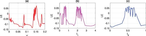
Figure 7. Lyapunov exponent diagrams corresponding to variations in system parameters, computed for a = 0.7, b = 0.6, $I_{1} = 2$, $k_{0} = 0.1$, $\sigma_{1} = 1.2$, $I_{2} = 0.5$, $\sigma_{2} = 0.5$, $a_{1} = \tfrac{1}{3}$, $\xi$ = 0.1, c = 0.1, $k_{1} = 0.8$, $k_{2} = 0.2$, a = 0.1, and $\beta$ = 0.2. Simulations were initiated from the initial condition $(0.1,\,0.2,\,0.1,\,0.2,\,0.1)$. (a) Lyapunov exponent plotted against $\omega$, (b) Lyapunov exponent plotted against I1, (c) Lyapunov exponent plotted against I2. |
Additionally, the various anger frequencies will influence choosing the electrical activity model; thus, the FHN neuron model should consider the various anger frequencies' values $\omega$. Figure 8 shows the estimated development of the energy function and action potential over time. In the chaotic state, we can also see that the two neurons' phase and effective energy are almost identical. The results presented in figures 9 and 10 clearly demonstrate that the behavior of the energy function in the FHN neuron model is strongly linked to the generation and propagation of action potentials. The energy function in the chaotic firing state demonstrates irregular and unpredictable fluctuations, with amplitudes that vary erratically over time. Unlike the structured oscillations observed in spiking or bursting regimes, chaotic dynamics produce a complex energy profile that reflects the underlying sensitivity of the system to initial conditions. According to this behavior, chaotic activity not only raises the degree of unpredictability in the amount of energy that is required, but it also has the potential to induce instability into the neural dynamics as a whole. There is a fundamental difference between the structured oscillatory profiles that are found in spiking and bursting states and the chaotic firing regime, which is characterized by irregular and non-periodic variations in the energy function. An indication of a relative stability of the system's energetic needs is the fact that the energy landscape goes through a significant drop throughout the shift from chaotic activity to a more structured bursting state. Instead, the energy function shows a sudden and irregular increase as the external forcing current is reduced, driving the system from chaotic or bursting activity into a quiescent state. This behavior points to a close link between neural excitability, changes in energy and external modulation and it also indicates that chaotic dynamics are particularly sensitive to parameter variations. To further examine this behavior, the average energy was calculated for different values of the input current, allowing the chaotic firing patterns to be characterized more clearly. This was done in order to better describe the quantitative assessment of the firing dynamics. For the representative case of $I_{1} = 0.6$ and $I_{2} = 0.6,$ the average energy was determined to be 3.6791, indicating the baseline energetic cost of sustaining irregular oscillatory activity. When the external currents were increased to $I_{1} = 1.2$ and $I_{2} = 0.8$, the system exhibited a higher value of 3.9919, reflecting the amplification of chaotic excitability under stronger stimulation. A further elevation of the input currents to $I_{1} = 1.8$ and $I_{2} = 1.2$ yielded an even larger energetic demand with the mean energy rising to 3.9655. The findings indicate a distinct correlation between the energy profile of chaotic firing and the intensity of external inputs, highlighting the close relationship between synaptic drive and the energetic expenditure of irregular neuronal activity.
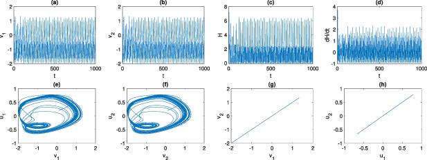
Figure 8. Dynamical evolution of the energy function and action potential under external stimulation. Subfigures (a) and (b) show the state variables v1 and v2, (c) shows the effective energy H, and (d) its time derivative $\dot{H}$. Phase-space trajectories are presented in (e)-(h). Simulations are performed for external currents $I_1 = 0.6$ and $I_2 = 0.6$, illustrating how the stimuli influence both the energy dynamics and neuronal firing behavior. |
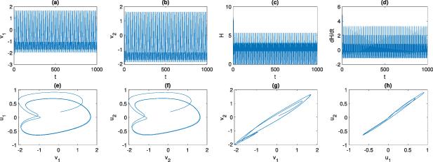
Figure 9. Dynamical evolution of the energy function and action potential under external stimulation. Subfigures (a) and (b) show the state variables v1 and v2, (c) shows the effective energy H, and (d) its time derivative $\dot{H}$. Phase-space trajectories are presented in (e)-(h). Simulations are performed for external currents $I_1 = 1.2$ and $I_2 = 0.8$, illustrating how the stimuli influence both the energy dynamics and neuronal firing behavior. |
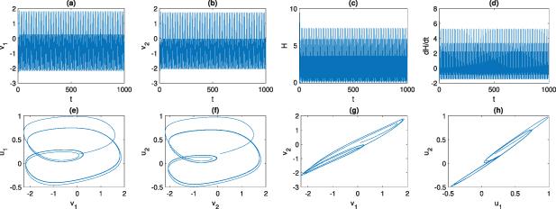
Figure 10. Dynamical evolution of the energy function and action potential under external stimulation. Subfigures (a) and (b) show the state variables v1 and v2, (c) shows the effective energy H, and (d) its time derivative $\dot{H}$. Phase-space trajectories are presented in (e)-(h). Simulations are performed for external currents $I_1 = 1.8$ and $I_2 = 1.2$, illustrating how the stimuli influence both the energy dynamics and neuronal firing behavior. |
One of the most valuable tools for demonstrating how the qualitative behavior of a nonlinear system shifts in response to changes in the value of a parameter is a bifurcation representation. The dynamical consequences of the externally delivered stimuli, which are described by the adjustable parameters identified as I1 and I2, are the primary focus of our investigation in this paper. Figure 11 shows the relevant bifurcation plot and dynamical map for model (2 ) when I1 and I2 systematically change from 0 to 4 and 0 to 2, respectively. We investigate how variations in these inputs shape the system's overall behavior. The bifurcation diagram is constructed by systematically examining the sequence of local maxima of the state variable $v_j, (j = 1,2)$. For the fixed excitation frequency $\omega$ = 0.15, chaotic dynamics are confined to a narrow interval of the amplitude parameters I1 and I2. With a further increase in these amplitudes, the chaotic regime ceases to persist, and the system transitions toward more regular and stable dynamical behaviors. With respect to the external drives, the applied current I1 was restricted to $1.2 \unicode{x2A7D} I_{1} \unicode{x2A7D} 3.0$, ensuring a sufficiently high excitation threshold capable of initiating complex firing sequences, whereas the second external input, I2, varied within $0.3 \unicode{x2A7D} I_{2} \unicode{x2A7D} 0.8$, which fine-tunes the oscillatory response and reinforces the transition into chaotic states. Collectively, these parameter intervals delineate the multidimensional domain in which chaotic firing modes persist, underscoring the delicate interplay between synaptic coupling and external forcing in shaping the nonlinear excitability of neuronal networks.
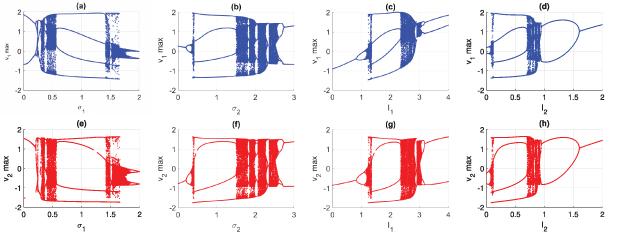
Figure 11. Bifurcation diagrams showing the maximum values of v1 and v2 for different system parameters. Subfigures (a)-(d) illustrate $v_1 \max$ versus $\sigma$1, $\sigma$2, I1, and I2, while subfigures (e)-(h) show $v_2 \max$ for the same parameters. These results demonstrate how changes in coupling strengths and external inputs influence the firing activity of the system. |
Furthermore, we display the coupling factor $\sigma$1 in order to demonstrate the many dynamical changes that occur in the coupled system when the coupling coefficient changes. In figure 11, we give the plots that depict the local maxima of the membrane potentials v1 and v2, which were obtained under the condition of a constant driving frequency of $\omega$ = 0.15. Within the coupling range of $ 0.5\unicode{x2A7D}\sigma_1\unicode{x2A7D}1.3$, we are capable of detecting coexisting chaotic attractors in both neurons. The secondary coupling strength, $\sigma$2, assumed values in the broader interval $0.4 \unicode{x2A7D} \sigma_{2} \unicode{x2A7D} 1.4$, thereby providing an additional modulatory influence contributing to the irregularity of spiking dynamics.
In this study, we performed numerical simulations of 201 independent realizations of neuronal action potentials to investigate the dynamical variability of the system, as shown in figure 12. The simulations were carried out by systematically varying the control parameter k0 within the interval $0 \unicode{x2A7D} k_{0} \unicode{x2A7D} 2$. To ensure statistical robustness, a Monte Carlo simulation framework was employed, where each realization represents a stochastic trial that captures potential variability in neuronal dynamics. This approach enables a comprehensive assessment of the influence of k0 on the generation and stability of action potentials, thereby providing deeper insights into the neuronal model's parameter-dependent excitability and firing patterns. The control parameter k0 was randomly sampled from a uniform distribution on the interval [0, 2], ensuring that each admissible value of k0 had equal probability of being selected. This stochastic sampling scheme, embedded within a Monte Carlo simulation, guarantees that the ensemble of realizations provides an unbiased statistical representation of the underlying neuronal dynamics. For each realization, the corresponding neuronal action potentials were recorded. Specifically, when the modulation frequency was fixed at $\omega$ = 0.005, we observed that the ensemble mean of the action potentials across all realizations attained statistically stable values for k0 lying within the interval $0.2 \unicode{x2A7D} k_{0} \unicode{x2A7D} 0.28$. This finding highlights that only a restricted subset of the parameter space yields consistent mean responses, underscoring the sensitivity of neuronal excitability to variations in k0. Similarly, when the modulation frequency was increased to $\omega$ = 0.015, the ensemble mean of the action potentials exhibited stable behavior only for k0 values within the interval $0.44 \unicode{x2A7D} k_{0} \unicode{x2A7D} 0.53$. This shift in the admissible parameter window concerning $\omega$ indicates a frequency-dependent modulation of the neuronal excitability, suggesting that higher driving frequencies require comparatively larger k0 values to sustain coherent action potential dynamics. Increasing the frequency to $\omega$ = 0.05 yielded a slightly narrower range of $0.41 \unicode{x2A7D} k_{0} \unicode{x2A7D} 0.50$, while for the higher frequency $\omega$ = 0.15, the admissible interval reverted to $0.23 \unicode{x2A7D} k_{0} \unicode{x2A7D} 0.28$. These observations indicate that the interaction between $\omega$ and k0 is non-monotonic, highlighting distinct frequency-dependent parameter windows in which neuronal excitability and coherent action potential generation are maintained.
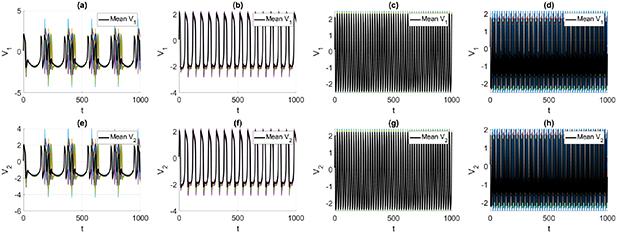
Figure 12. Firing patterns from 201 random simulations of parameter k0 are shown in subfigures (a)-(h), corresponding to eight different conditions. In each subfigure, the colored traces represent the individual Monte Carlo realizations, while the solid black line highlights the mean firing response across all simulations. |
3.2.2. Influence of external magnetic noise on the coupling system.
In realistic electromagnetic settings, magnetic fields are naturally affected by random fluctuations caused by environmental disturbances and inherent electromagnetic noise. Because neuronal interactions in the present model occur through a magnetic-flux-dependent coupling variable, these fluctuations mainly influence the coupling pathway rather than the neurons' intrinsic dynamics. To account for this effect, external magnetic noise is explicitly introduced into the coupling system by modifying the magnetic coupling equation as
$\begin{align} \dot{\phi} = k_1\left(v_1-v_2\right) -k_2\phi + \sigma_m \zeta\left(t\right),\end{align}$
where $\zeta(t)$ represents Gaussian white noise with zero mean and unit variance, and $\sigma$m controls the noise intensity. It is important to note that the neuronal state equations and the external excitation are kept unchanged. This formulation isolates the effect of external magnetic field fluctuations on the coupling mechanism, allowing a systematic and physically meaningful assessment of the robustness of the coupled system under noisy electromagnetic conditions.To provide additional insight into the influence of external magnetic noise on the coupling system, we investigate its interplay with the frequency of the external periodic excitation. Figure 13 depicts the synchronization error for four representative values of the driving frequency $\omega$, with each panel comparing different magnetic noise intensities. The results reveal that the effect of magnetic noise is strongly dependent on the excitation frequency. At low excitation frequencies, the coupling mechanism is able to suppress noise-induced disturbances, leading to stable and reliable synchronization. As the frequency increases, however, magnetic noise produces stronger fluctuations and slows down the synchronization process, indicating that the coupling becomes more sensitive. These results show that the effect of external magnetic noise depends strongly on the excitation frequency and has an important influence on the coupling dynamics under periodic stimulation.

Figure 13. Influence of external magnetic noise on the coupling system for different excitation frequencies show the time evolution of the synchronization error $\mid v_1 - v_2 \mid$: (a) $\omega$ = 0.005, (b) $\omega$ = 0.015, (c) $\omega$ = 0.05, and (d) $\omega$ = 0.15. Each subplot illustrates the $\mid v_1 - v_2 \mid$ dynamics corresponding to a specific external stimulation frequency, demonstrating the transition across distinct firing regimes, when $I_1 = 1.8 ~\&~ I_2 = 1.2$. In each panel, curves correspond to three magnetic noise intensities σm, illustrating the frequency-dependent sensitivity of the coupling system to external magnetic noise. |
3.2.3. Synchronous stability of the coupling system.
The synchronous state of the coupling system corresponds to identical neuronal dynamics, characterized by $v_1(t) = v_2(t)$ and $u_1(t) = u_2(t)$. In this state, both neurons evolve on the same trajectory, and the system dynamics are confined to the synchronous manifold. Synchronous stability refers to the system's ability to maintain its synchronous state when subjected to small perturbations. In other words, once synchronization is achieved, the synchronous manifold is considered stable if minor deviations decay over time and the system returns to synchronized motion.
To analyze the stability of the synchronous state, synchronization error variables are introduced as
$\begin{align} e_v = v_1 -v_2, ~~~~e_u = u_1 - u_2,\end{align}$
which quantify deviations from the synchronous manifold in the voltage and recovery variables, respectively.In addition, the synchronization function is defined as
$\begin{align} e\left(t\right) = \sqrt{e_v^2 + e_u^2},\end{align}$
which represents the total deviation from synchrony. The decay of e(t) toward zero indicates asymptotic stability of the synchronous state.Numerical simulations are performed by introducing small perturbations in the initial conditions of the coupled neurons while keeping all system parameters identical. The subsequent evolution of the error variables and the synchronization function is monitored to assess the stability of the synchronous manifold. Figures 14(a)-(d) illustrates the dynamical evolution of synchronous stability through the time series of the synchronization error e(t) as a control parameter is varied. In figure 14(a), the error remains bounded with intermittent peaks, indicating a stable but imperfect synchronous state in which the system trajectories stay close to the synchronous manifold except during brief spiking events. The presence of these sporadic peaks signifies that while there is some degree of stability, the impact of transient disturbances cannot be overlooked, as they interrupt the otherwise harmonious synchrony among the system's components. As the parameter increases (figure 14(b)), the error exhibits regular and periodic bursts while maintaining a low baseline, signifying stable phase synchronization where the neurons remain phase-locked despite amplitude mismatch. This phenomenon highlights the resilience of the system, showcasing how the impact of consistent periodicity allows the neurons to achieve a synchronized state, even in the presence of differentiation in signal amplitudes. The steady low baseline of the synchronization error during this phase emphasizes the robust nature of the synchronized dynamics under specific conditions. With further parameter variation (figure 14(c)), the error becomes dense and rapidly fluctuating, characterizing a transition regime associated with weakened synchronous stability and the breakdown of phase locking. This depicts a significant impact on the overall coherence of the system, as fluctuations begin to dominate, leading to a loss of the stability once observed. Such instability is indicative of a critical threshold being crossed, suggesting that the system is moving towards a more chaotic and unpredictable state. Finally, in figure 14(d), the error displays persistent high-amplitude irregular oscillations without approaching zero, demonstrating a complete loss of synchronous stability and the emergence of fully desynchronized dynamics. The impact of this complete desynchronization reveals a profound shift from order to chaos, effectively illustrating how slight variations in control parameters can precipitate dramatic changes in system behavior. Overall, these results reveal a clear dynamical transition from stable synchronous behavior to instability mediated by intermittent and phase-synchronized regimes, marking an essential understanding of synchronization processes and their delicate balance within complex systems. Notably, when the control parameters satisfy $I_1 = I_2$, the synchronization error converges to zero, confirming the existence of complete synchronization.
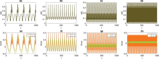


Figure 14. Time series demonstrating synchronous stability for different values of the control parameter. Panels (a)-(d) show the synchronization error e(t), while panels (e)-(h) display the corresponding state differences $v_1-v_2$ and $u_1-u_2$ for the same parameter values. The figure illustrates the transition from stable synchronization to complete desynchronization. |
4. Conclusion
In the study, a chaotic non-autonomous network system was developed. The network could display periodic, chaotic spiking-bursting firings, according to numerical simulations. The energy variety in a homogeneous two-neuron network and the energy variations of neurons during periodic, chaotic spiking-bursting firings could be shown using the FHN model's effective energy function, which was obtained using Helmholtz's theorem. It was shown that when the membrane potentials of the two neurons change, the memristor synapse activates and functions as a coupling channel to transfer energy, hence enhancing energy variety and resulting in the emergence of complex dynamical behaviors. The starting state and coupling strength could be used to change the energy communicated by the memristor synapse, allowing the two neurons to achieve perfect synchronization and energy balance. These findings have biophysical significance because they show that neurons from various functional regions rarely aim to fire at the same speed. Instead, they are controlled to maintain a high degree of energy balance, allowing different functional neurons to choose the best firing modes for the nervous system. For the future use of intelligent sensors and precise signal recognition in noisy environments, these findings provide helpful direction. In conclusion, the present study systematically demonstrates that synchronous stability is strongly governed by control-parameter matching, with complete synchronization emerging when $I_1 = I_2$, whereas increasing mismatch drives a clear dynamical transition toward desynchronized states.