Welcome to visit Communications in Theoretical Physics,
Mathematical Physics

Traveling waves, modulational instability and routes to chaos in a stochastic non-Boussinesq wavepacket model

  • Ahmed H Arnous 1, 2 ,
  • Muhammad Naveed Rafiq 3 ,
  • Muhammad Hamza Rafiq , 4, 5, *
Expand
  • 1Department of Mathematical Sciences, Saveetha School of Engineering, SIMATS, Chennai 602105, Tamilnadu, India
  • 2Research Center of Applied Mathematics, Khazar University, Baku AZ-1096, Azerbaijan
  • 3School of Mathematics and Statistics, Central South University, Changsha 410083, China
  • 4Department of Physics, Zhejiang Normal University, Jinhua 321004, China
  • 5Center for Theoretical Physics, Khazar University, 41 Mehseti Str., Baku AZ1096, Azerbaijan

*Author to whom any correspondence should be addressed.

Received date: 2025-11-10

  Revised date: 2026-05-08

  Accepted date: 2026-05-08

  Online published: 2026-06-16

Copyright

© 2026 Institute of Theoretical Physics CAS, Chinese Physical Society and IOP Publishing. All rights, including for text and data mining, AI training, and similar technologies, are reserved.
This article is available under the terms of the IOP-Standard License.

Abstract

This paper develops a stochastic variant of the non-Boussinesq wavepacket model, an nonlinear Schrödinger (NLS) type envelope description for internal wave packets in strongly stratified media. Multiplicative Stratonovich noise is introduced in the carrier phase to represent environmental fluctuations. A gauge transformation with a traveling wave reduction yields a deterministic Hamiltonian envelope system that admits periodic wavetrains, localized pulse profiles, and kink type fronts across relevant parameter regimes. A modulational instability analysis identifies the sideband growth condition and shows how higher order dispersion shifts the unstable band, while phase noise does not change the leading growth rate. To probe complexity under weak periodic forcing, a Melnikov analysis predicts transverse manifold intersections and the onset of chaotic dynamics, supported by numerical sections, bifurcation diagrams, and Lyapunov exponents. The framework links stochastic modeling and nonlinear wave dynamics and provides practical diagnostics for stability, coherence, and complexity in non Boussinesq media and in related NLS type systems.

Cite this article

Ahmed H Arnous , Muhammad Naveed Rafiq , Muhammad Hamza Rafiq . Traveling waves, modulational instability and routes to chaos in a stochastic non-Boussinesq wavepacket model[J]. Communications in Theoretical Physics, 2026 , 78(8) : 085004 . DOI: 10.1088/1572-9494/ae6a7a

1. Introduction

The non-Boussinesq wavepacket (NBWP) model is a higher-order nonlinear Schrödinger (NLS)-type envelope equation tailored for internal wave packets in strongly stratified media, precisely where the classical Boussinesq approximation breaks down [1-3]. In stratified fluids, the Boussinesq approximation assumes density variations are negligible except in the buoyancy term; this is accurate only when the relative density variation is small. In strongly stratified environments, relaxing this assumption leads to several physically observable non-Boussinesq signatures. The effective inertia and buoyancy restoring forces become depth- and amplitude-dependent, which modifies the dispersion relation and the phase and group velocities of internal waves. Waveform asymmetry can increase, with sharper crests or fronts and altered polarization relations compared with Boussinesq predictions. Energy flux and momentum transport are modified because density variations enter the kinetic energy and pressure work budgets, influencing the conditions for wave steepening, breaking, and mixing. These effects motivate the use of non-Boussinesq envelope descriptions for internal wave packets in the ocean and atmosphere, where accurate prediction of transport and onset of breaking requires going beyond classical Boussinesq reductions [1, 2, 4, 5]. It belongs to the NLS-type family of models but incorporates non-Boussinesq effects, making it more accurate for situations with strong density variations, such as atmospheric and oceanic dynamics [4, 5]. Viewed through the lens of dynamical systems and bifurcation theory, the model supports families of exact traveling waves-solitary pulses, periodic wavetrains, and kink-type fronts-that organize the qualitative pathways of nonlinear wave propagation and energy transport [6-8].
This model is significant because it connects mathematical theory with physical applications. It has strong links to the NLS equation, which is widely applied in nonlinear optics, plasma physics, photonics, Bose-Einstein condensates, and condensed matter physics [9-13]. In geophysical fluid dynamics, the non-Boussinesq form is essential for predicting the behavior of internal ocean and atmospheric waves, where it helps explain energy transport, wave breaking, and mixing [14, 15]. Accordingly, the NBWP framework offers a unifying envelope description across disparate physical settings while retaining the additional dispersion and derivative nonlinearities needed for fidelity in strongly stratified flows. Its study not only advances theoretical understanding but also provides practical tools for analyzing complex nonlinear systems across physics and engineering [16, 17].
Moreover, introducing stochastic perturbations in the Stratonovich sense provides both motivation and novelty. In realistic physical environments, wave dynamics are influenced by random fluctuations such as turbulence, background noise, or external forcing. The Stratonovich framework is natural in this context because it preserves standard calculus rules and corresponds to the physics of continuously varying noisy inputs [7, 18]. In particular, multiplicative phase noise represents broadband environmental variability acting on the carrier, and, importantly for analysis, it admits a gauge transformation that eliminates the noise from the amplitude dynamics. This observation clarifies which stability and coherence properties remain robust under noise and which are modified by higher-order dispersive effects. Extending the deterministic NBWP model to its stochastic counterpart makes it possible to examine how noise influences the stability, persistence, and bifurcation of solitary, periodic, and kink solutions. This positions our study at the intersection of stochastic analysis and nonlinear wave dynamics, with implications for climate and ocean applications as well as for NLS-type systems in optics and condensed matter.
Internal wave packets propagate through environments that are not perfectly stationary. Background turbulence, intermittent shear, mesoscale variability, slowly varying stratification, and topographic interactions can introduce random fluctuations in the carrier phase and coherence of the packet. At the envelope level, such unresolved variability can be represented by stochastic perturbations that capture random phase wandering and loss of phase coherence, variability in interference and cross correlation phase lags used in observations, and run to run variability in modulation timing. We adopt multiplicative Stratonovich phase noise because it is consistent with continuously varying physical perturbations and preserves the standard chain rule, allowing an exact random gauge transformation. This enables separation of deterministic amplitude dynamics that govern modulation instability, coherent structure regimes, and forced transitions from stochastic phase variability, which clarifies which diagnostics are robust to phase noise and which become realization dependent [7, 18].
Existing envelope models for internal waves often rely on Boussinesq-based reductions or lower-order NLS-type approximations, which can under-represent higher-order dispersive and derivative nonlinear effects that are relevant in strongly stratified regimes. On the other hand, stochastic extensions frequently treat noise in a generic way, without isolating which stability predictions are fundamentally altered by randomness and which remain controlled by the deterministic dispersion and nonlinearity balance. The objective of this work is to address both points within a single NBWP framework. We retain the higher-order dispersive structure needed for non-Boussinesq fidelity, and we introduce a physically interpretable Stratonovich phase-noise term that is exactly reducible by a random gauge. This yields a tractable route to Hamiltonian traveling-wave classification, explicit MI growth-rate predictions showing how higher-order dispersion shifts the unstable band, and threshold-type criteria for the onset of irregular modulation under weak deterministic forcing, thereby linking model structure to observable coherence, instability, and complexity in stratified environments.
Beyond their foundational role in nonlinear wave theory, soliton-like structures and coherent localized waveforms are increasingly linked to concrete applications in fluids and photonics. In fluid mechanics, controlled cavitation-bubble collapse can generate strongly localized impulsive dynamics that has been exploited for micro-scale launching and actuation [19]. In photonics, soliton formation in engineered lattices such as photonic moiré structures provides robust localization and rich propagation dynamics that can be tuned by the underlying lattice modulation [20]. Moreover, fractional generalizations and higher-order NLS systems support unconventional soliton families and reveal how nonlocality and higher-order dispersion reshape waveform morphology and stability characteristics [21]. These recent developments motivate envelope models that retain higher-order dispersive physics and incorporate environmental variability, since both ingredients can be decisive in realistic propagation environments and in predicting transitions from coherent wavepackets to complex modulation.
We therefore consider the following stochastic higher-order NLS-type model [3], obtained by incorporating a Stratonovich multiplicative noise term into the carrier phase:
$\begin{align} &\mathrm{i}\,\mathrm{d}u+\left\{u_{xx}-2\delta\beta|u|^{2}u - \mathrm{i}\,u_x + \mathrm{i}\,\alpha\,u_{xxx}- \mathrm{i}\,\left(|u|^{2}\right)_x\,u\right\}\nonumber\\ &\quad \times \mathrm{d}t = \sigma\,u\circ \mathrm{d}W\left(t\right).\end{align}$
In equation (1) we introduce stochasticity through a multiplicative phase term in the Stratonovich sense. This choice is deliberate. It provides a minimal representation of fast environmental variability that predominantly randomizes the packet phase while preserving a random gauge structure that allows an exact reduction to a deterministic envelope equation for the gauged field. This, in turn, enables a systematic phase plane classification, modulational instability (MI) analysis, and forced chaos diagnostics within a single analytical framework.
The stochastic NBWP equation (1) provides a physically consistent envelope model for internal wave packets in strongly stratified non-Boussinesq environments, where classical Boussinesq reductions are inadequate. Including multiplicative Stratonovich phase noise captures broadband environmental variability while preserving the standard calculus structure of the underlying physics. From an applications viewpoint, the model supports predictive analysis of coherence and localization of internal wave packets, which are relevant to energy transport, mixing, and wave breaking in geophysical flows, and stability to complexity transitions under weak external forcing. From a broader perspective, because the NBWP model is a higher-order NLS type envelope, the analytical and dynamical systems diagnostics developed here, including traveling wave classification, MI criteria, and chaos predictors, are transferable to related NLS type settings in nonlinear optics and condensed matter contexts.
In equation (1), $u = u(x,t)$ is the complex wave envelope, ux and uxx denote first- and second-order spatial derivatives, and uxxx represents the third-order dispersion term. The parameters δ and β characterize the strength of cubic nonlinear interactions, while a accounts for higher-order dispersion effects. The stochastic term $\sigma\,u\circ \mathrm{d}W(t)$ introduces multiplicative noise in the Stratonovich sense, where σ > 0 measures the noise intensity and W(t) is a standard Wiener process modeling random fluctuations. The linear convective term $-\mathrm{i}\,u_x$ and the self-steepening contribution $-\mathrm{i}\,(|u|^{2})_x u$ capture, respectively, group-velocity advection and nonlinear wavefront sharpening. Altogether, this formulation generalizes the deterministic model to capture both nonlinear wave dynamics and stochastic influences. By means of a gauge transformation combined with a traveling-wave reduction, we obtain a deterministic Hamiltonian envelope system admitting periodic wavetrains, localized pulses, and kink-type fronts. A MI analysis reveals the sideband growth condition in terms of effective group-velocity dispersion (GVD) and cubic nonlinearity and shows that higher-order dispersion shifts the unstable band, while phase noise leaves the leading growth rate unchanged. Finally, under weak periodic forcing we establish, via Melnikov theory [22, 23] and numerical diagnostics (Poincaré sections, bifurcation diagrams, Lyapunov exponents), routes to chaos in the reduced dynamics [24, 25].
On the deterministic side, the NBWP framework extends earlier non-Boussinesq internal-wavepacket models and validations in strongly stratified media by retaining higher-order dispersive and derivative nonlinear effects that are needed for accurate envelope dynamics beyond classical Boussinesq reductions [1, 2]. Quantitatively, our MI analysis provides explicit sideband growth rates and shows how the third-order dispersion parameter shifts the unstable band, giving a concrete dispersion-controlled correction to the instability window.
On the stochastic side, recent studies of stochastic NLS-type equations typically investigate how random perturbations modify solution statistics, stability diagnostics, and bifurcation scenarios [7, 8]. In contrast, the present model introduces Stratonovich multiplicative phase noise for which a random gauge transformation removes the explicit noise from the amplitude equation; therefore, the leading MI growth rate coincides with that of the reduced deterministic envelope, while the physical field retains realization-dependent phase modulation. This clarifies, in a quantitative way, which spectral-stability predictions are governed by deterministic dispersion/nonlinearity balance and which features (phase coherence, ensemble variability) are influenced by the stochastic phase factor.
Recent studies have explored bifurcations, chaotic dynamics, and sensitivity diagnostics together with novel soliton constructions in a variety of nonlinear wave models, including fractional solitary-wave systems with bifurcation and chaos analysis [26], fractional and higher-dimensional transmission-line models with nonlocal derivatives [27], shallow-water equations involving multi-soliton solutions, chaos, and sensitivity analysis [28], extended KP-type equations and KP hierarchy generalizations, including lumps, breathers, and rogue waves [29, 31], stochastic symmetry reductions in nonlinear metamaterial models [30], and comparative investigations of solitary waves, bifurcation structure, and chaos within stochastic dynamical systems [32]. While these works provide valuable benchmarks for dynamical-systems diagnostics and exact-wave construction in optics-inspired or KP-type frameworks, the present manuscript differs in modeling target and mechanism. We study a stochastic NBWP envelope relevant to strongly stratified media, where the stochasticity enters as Stratonovich multiplicative phase noise that is exactly removable by a random gauge. Accordingly, we classify coherent structures via the reduced Hamiltonian traveling-wave system, derive explicit MI growth rates governed by the effective dispersion and nonlinearity of the NBWP envelope, and quantify transitions to irregular modulation under weak forcing through a Melnikov threshold and numerical chaos diagnostics. This provides a unified stability-to-complexity comparison framework tailored to NBWP dynamics, complementing the optical, KP, and fractional settings emphasized in [26-32].

2. Analytical derivation

It is important to distinguish between the dynamics of the transformed variable and the dynamics of the physical field. Because the noise enters equation (1) as a Stratonovich multiplicative phase term, the gauge change of variables
$equation*$
(with the appropriate coefficient and sign as in equation (1)) is legitimate under the ordinary (Stratonovich) chain rule and converts the SPDE into a deterministic PDE for $\tilde u(x,t)$. Nevertheless, the physical field $u(x,t)$ remains a stochastic process, since it is obtained by the inverse map involving the Wiener path Wt. Thus, the reduced equation for $\tilde u$ is deterministic, but the physical solution family $\{u(\cdot,\cdot;\omega)\}$ is random through the multiplicative factor $\exp(\mathrm{i}\sigma W_t(\omega))$. In particular, phase-sensitive observables exhibit realization-to-realization variability, while modulus-based quantities may remain unchanged (or change only through parameter or initial-data randomness if introduced). Accordingly, our reduction should be interpreted as an exact random gauge equivalence: the SPDE is not replaced by a different stochastic model, but rewritten in a form where the stochasticity is carried explicitly by the gauge factor and the remaining evolution is deterministic.
To eliminate the Stratonovich multiplicative noise from the phase, we apply a gauge-type transformation. Substituting the traveling-wave ansatz
$u(x, t)=\Omega(\eta) \mathrm{e}^{\mathrm{i}(-\kappa x+\omega t-\sigma W(t))}, \quad \eta=x-v t$
and separating real and imaginary parts yields
$\begin{align} \text{Re:}\quad &-\left(\kappa+\kappa^2+\alpha\kappa^3+\omega\right)\,\Omega\left(\eta\right)\;-\;2\beta\delta\,\Omega\left(\eta\right)^3 \;\nonumber\\ &\quad +\;\left(1+3\alpha\kappa\right)\,\Omega^{^{\prime\prime}}\left(\eta\right) = 0,\end{align}$
$\begin{align} \text{Im:}\quad &-\left(1+v+2\kappa+3\alpha\kappa^2\right)\,\Omega^{^{\prime}}\left(\eta\right)\;-\;2\,\Omega\left(\eta\right)^2\,\Omega^{^{\prime}}\left(\eta\right) \;\nonumber\\ &\quad+\;\alpha\,\Omega^{\left(3\right)}\left(\eta\right) = 0.\end{align}$
Integrating (4) once with respect to η, and setting the integration constant to zero (consistent with localized or decaying envelopes), yields
$\begin{align} \left(-1-v-2\kappa-3\alpha\kappa^2\right)\,\Omega\left(\eta\right)\;-\;\frac{2}{3}\,\Omega\left(\eta\right)^3 \;+\;\alpha\,\Omega^{^{\prime\prime}}\left(\eta\right) = 0.\end{align}$
Matching the structures of (3) and (5) enforces the following consistency relations:
$\begin{align} \frac{\kappa+\kappa^2+\alpha\kappa^3+\omega}{\,1+v+2\kappa+3\alpha\kappa^2\,} \; = \;3\beta\delta \; = \;\frac{1+3\alpha\kappa}{\alpha}.\end{align}$
The relations in (6) are consistency conditions ensuring that the real part (3) and the integrated imaginary part (5) reduce to the same stationary envelope ODE. Thus, (6) does not restrict the full PDE dynamics; it selects a coherent traveling-wave branch for which the reduction to (7) is exact.
Moreover, (6) can be used constructively: from
$3 \beta \delta=\frac{1+3 \alpha \kappa}{\alpha}=\frac{1}{\alpha}+3 \kappa$
we obtain the explicit relation
$\kappa=\beta \delta-\frac{1}{3 \alpha}, \quad(\alpha \neq 0)$
Then, choosing any admissible wave speed v (avoiding degeneracy) determines the frequency $\omega$ from the remaining equality in (6) as
$\begin{align*} \omega = 3\beta\delta\left(1+v+2\kappa+3\alpha\kappa^{2}\right)-\left(\kappa+\kappa^{2}+\alpha\kappa^{3}\right),\end{align*}$
provided the denominators in (6) are nonzero:
$1+3 \alpha \kappa \neq 0, \quad 1+\nu+2 \kappa+3 \alpha \kappa^{2} \neq 0 .$
Hence, (6) leaves a nontrivial admissible set and provides a transparent parameter-selection rule.
Under (6), the envelope $\Omega(\eta)$ satisfies the single second-order nonlinear ODE
$\chi_{1} \Omega(\eta)+\chi_{2} \Omega(\eta)^{3}+\Omega^{\prime \prime}(\eta)=0,$
where
$\begin{align} \begin{cases} \chi_1 = -\dfrac{\kappa+\kappa^2+\alpha\kappa^3+\omega}{1+3\alpha\kappa}, \\[6pt] \chi_2 = -\dfrac{2\beta\delta}{1+3\alpha\kappa}. \end{cases}\end{align}$
Equation (7) represents the standard stationary envelope equation, from which localized traveling-wave solutions (e.g. bright or dark) can be constructed, depending on the signs of χ1 and χ2.
The reduction above provides a deterministic envelope equation and establishes the sign conventions for $(\alpha,\beta,\delta)$. We now employ the same gauge and co-moving frame to investigate the MI of the associated uniform wavetrain.

2.1. Modulational instability (MI)

We examine the modulational (Benjamin-Feir) stability [33] of a uniform wavetrain in the stochastic higher-order NLS-type model. The Stratonovich multiplicative noise can be gauged out of the phase by the transformation
$u(x, t)=v(x, t) \mathrm{e}^{-\mathrm{i} \sigma W(t)} .$
By Stratonovich calculus, this removes the explicit noise from the amplitude dynamics. Hence modulational growth rates are computed from the deterministic equation satisfied by v:
$\mathrm{i} v_{t}+v_{x x}-2 \delta \beta|v|^{2} v+\mathrm{i} \alpha v_{x x x}-\mathrm{i}\left(|v|^{2}\right)_{x} v-\mathrm{i} v_{x}=0$
Working in the co-moving frame $\xi = x+t$ (which removes the linear convective term $ -\mathrm{i} v_x$), we set $v(\xi,t)\to V(\xi,t)$ and for simplicity, relabel $V (\xi, t)$ as $v(\xi, t)$. Thus the reduced deterministic envelope equation used for the MI calculation is
$\mathrm{i} v_{t}+v_{\xi \xi}-2 \delta \beta|v|^{2} v+\mathrm{i} \alpha v_{\xi \xi \xi}-\mathrm{i}\left(|v|^{2}\right)_{\xi} v=0 .$
We then consider the uniform wavetrain
$v_{0}(\xi, t)=A \mathrm{e}^{\mathrm{i}(Q \xi-\Omega t)}, \quad A>0, Q \in \mathbb{R} .$
Substitution of (11) into (9) gives the carrier frequency
$\Omega=Q^{2}-\alpha Q^{3}+2 \delta \beta A^{2}$
To probe sideband stability, perturb the carrier by a pair of symmetric Fourier sidebands:
$v(\xi, t)=\left[A+\varepsilon\left(a \mathrm{e}^{\mathrm{i}(k \xi-\lambda t)}+b \mathrm{e}^{-\mathrm{i}(k \xi-\lambda t)}\right)\right] \mathrm{e}^{\mathrm{i}(Q \xi-\Omega t)}+O\left(\varepsilon^{2}\right)$
with $0 \lt |k|\ll 1$. Linearizing (9) yields a $2\times2$ spectral problem for (a, b) whose dispersion relation can be written in a compact long-wave (Whitham) form:
$\lambda^{2}=2 P_{\mathrm{eff}}(Q) Q_{\mathrm{eff}} A^{2} k^{2}-P_{\mathrm{eff}}(Q)^{2} k^{4}+O\left(k^{3}\right) .$
Here,
$\begin{align} P_{\mathrm{eff}}\left(Q\right) = \tfrac12\,\omega^{^{\prime\prime}}_{\mathrm{lin}}\left(Q\right) = 1-3\alpha Q, \qquad \omega_{\mathrm{lin}}\left(q\right) = q^2-\alpha q^3,\end{align}$
is the effective GVD at the carrier, and
$Q_{\mathrm{eff}}=-2 \delta \beta,$
is the effective cubic nonlinearity (with the sign convention of (9)). The derivative nonlinearity $ -i(|v|^2)_x v $ and third-order dispersion $ \alpha v_{xxx} $ generate higher-order (odd in k) skew terms that shift the spectral peak and break the $k\mapsto -k$ symmetry but do not alter the leading k2 and k4 coefficients in (13).
The dispersion relation (12) is obtained by the classical sideband linearization applied to the reduced NBWP envelope equation; in this sense, its algebraic structure is consistent with the standard MI calculation for higher-order NLS-type models. The contribution here is not the existence of a Whitham expansion by itself, but the NBWP-specific interpretation and its coupling to the stochastic modeling: because the original SPDE contains Stratonovich multiplicative phase noise that is exactly removable by a random gauge, the leading MI exponent predicted by (12) coincides with that of the deterministic reduced envelope, while the physical field retains realization-dependent phase modulation. Moreover, (12) provides an explicit parameter-resolved map of how higher-order dispersion shifts the unstable sideband interval and the maximally amplified perturbation scale, which we use to delineate coherence versus breakup regimes and to connect instability-driven modulation to the subsequent forced-dynamics (bifurcation and chaos) diagnostics.
MI criterion and gain. From (13), MI occurs when
$\begin{equation} P_{\mathrm{eff}}\left(Q\right)\,Q_{\mathrm{eff}} \; \gt \; 0 \quad\Longleftrightarrow\quad \left(1-3\alpha Q\right)\,\left(-2\delta\beta\right)\; \gt \;0.\end{equation}$
In this case the unstable band is, to leading order,
$0<k^{2}<2 \frac{Q_{\mathrm{eff}}}{P_{\mathrm{eff}}(Q)} A^{2}, \quad \frac{Q_{\mathrm{eff}}}{P_{\mathrm{eff}}(Q)}>0$
and the real growth rate is
$g(k)=\Re \lambda(k) \approx|k| \sqrt{2 P_{\mathrm{eff}}(Q) Q_{\mathrm{eff}} A^{2}-P_{\mathrm{eff}}(Q)^{2} k^{2}} .$
The most unstable wavenumber and the peak gain follow immediately:
$\begin{equation} k_*^2 = \frac{Q_{\mathrm{eff}}}{P_{\mathrm{eff}}\left(Q\right)}\,A^2, \qquad g_{\max} = |Q_{\mathrm{eff}}|\,A^2 = 2\,|\delta\beta|\,A^2,\end{equation}$
showing that (to leading order) the TOD parameter a shifts the peak location via $P_{\mathrm{eff}}(Q)$ while the peak height depends only on the cubic nonlinearity and the carrier amplitude.
The MI growth rate reported here is derived from the deterministic evolution equation satisfied by the gauged field $u(x,t)$ obtained after the Stratonovich random phase transformation. Consequently, the leading-order MI gain is controlled by the effective dispersion and nonlinearity coefficients of the reduced deterministic model and is not altered by the Stratonovich multiplicative phase noise term in equation (1).
In the original variables, the physical field is $u(x,t) = \tilde u(x,t)\exp(\mathrm{i}\sigma W_t)$, so the noise contributes a realization-dependent global random phase modulation. This affects phase-sensitive diagnostics (for example, coherence and interference-type measures) and may influence ensemble-averaged observables, but it does not change the deterministic exponential sideband-amplitude growth rate that defines the classical MI spectrum computed from $\tilde u$. Accordingly, throughout this paper the MI results should be interpreted as intrinsic spectral stability properties of the underlying NBWP envelope dynamics, with the stochasticity entering through a random phase factor rather than through a modification of the MI exponent itself.

3. Hamiltonian structure and phase-plane geometry

The study of nonlinear dynamical systems is central to contemporary applied mathematics, physics, and engineering because it reveals how simple models can generate rich behaviors such as bifurcations, quasi-periodic motion on invariant tori, and chaos [22-25]. In [3], Wang et al systematically analyzed the nonlinear dynamics of dynamical systems via bifurcation theory, demonstrating how qualitative behavior varies with system parameters. In line with this literature, we begin with the unforced, undamped cubic oscillator and its Hamiltonian (conservative) dynamics. The effects of weak periodic forcing and damping (which are responsible for transitions from periodic motion to quasi-periodic tori and, ultimately, chaos as the forcing amplitude increases) will be addressed in a later section [34]. The two-dimensional Hamiltonian system associated with the cubic nonlinear oscillator (cf (7)) is
$\begin{equation} \begin{cases} \dfrac{\mathrm{d}\Omega}{\mathrm{d}\eta} = \phi,\\[6pt] \dfrac{\mathrm{d}\phi}{\mathrm{d}\eta} = -\,\chi_1\Omega-\chi_2\Omega^3. \end{cases}\end{equation}$
Equivalently, this is a canonical Hamiltonian system with $\dfrac{\mathrm{d} \Omega}{\mathrm{d}\eta} = \dfrac{\partial \mathscr{H}}{\partial \phi}$ and $\dfrac{\mathrm{d}\phi}{\mathrm{d}\eta} = -\dfrac{\partial \mathscr{H}}{\partial \Omega}$, confirming its conservative structure. Multiplying the second-order equation by $\Omega^{^{\prime}}(\eta)$ and integrating once yields the conserved energy (Hamiltonian)
$\mathscr{H}(\Omega, \phi)=\frac{1}{2} \phi^{2}+\frac{\chi_{1}}{2} \Omega^{2}+\frac{\chi_{2}}{4} \Omega^{4}=H$
where H is the constant total energy determined by the initial conditions and $\dfrac{\mathrm{d}\mathscr{H}}{\mathrm{d}\eta} = 0$ along trajectories. The function
$V(\Omega)=\frac{\chi_{1}}{2} \Omega^{2}+\frac{\chi_{2}}{4} \Omega^{4},$
acts as an effective potential, while $\tfrac{1}{2}\phi^2$ is the kinetic energy. Because $\nabla_{(\Omega,\phi)}\!\cdot(\phi,\,-\chi_1\Omega-\chi_2\Omega^3) = \dfrac{\partial \phi}{\partial \Omega}+\dfrac{\partial (-\chi_1\Omega-\chi_2\Omega^3)}{\partial \phi} = 0$, the flow is area-preserving, and trajectories are confined to the level sets of $\mathscr{H}$: no attractors or limit cycles occur in this conservative setting (Poincaré-Bendixson arguments). Depending on the shape of V, phase portraits display closed periodic orbits around centers, separatrices forming homoclinic loops, or heteroclinic connections between distinct saddles [35].
We note that the reduced traveling-wave dynamics takes the form of a quartic (Duffing-type) oscillator, whose generic phase-portrait geometry and equilibrium classification are well documented in the dynamical-systems literature. The role of the present reduction is therefore not to re-establish the abstract Duffing taxonomy, but to provide an explicit NBWP-to-Duffing parameter map: the coefficients of the quartic potential and the associated Hamiltonian level sets are expressed in closed form in terms of the NBWP physical parameters (wave speed, higher-order dispersion, and nonlinear coefficients) subject to the matching conditions. This mapping yields model-specific existence criteria for homoclinic and heteroclinic connections (localized pulses and kink or front profiles) and identifies admissible parameter regimes in which such coherent structures can occur in the NBWP setting.

3.1. Equilibria, linearization, and local orbit classification

Equilibria satisfy $\phi^* = 0$ and $-\chi_1\Omega^*-\chi_2(\Omega^*)^3 = 0$, i.e.
$\begin{equation*} \left(\Omega^*,\phi^*\right) = \left(0,0\right), \quad \left(\Omega^*,\phi^*\right) = \left(\pm\sqrt{\tfrac{-\chi_1}{\chi_2}},\,0\right) \quad\text{(when}~\chi_1\chi_2 \lt 0\text{)}.\end{equation*}$
The Jacobian reads
$\begin{align*} & J\left(\Omega,\phi\right) = \begin{bmatrix} 0 & 1\\[4pt] -\chi_1-3\chi_2\Omega^2 & 0 \end{bmatrix},\nonumber\\ & \quad \text{so the eigenvalues at}~\left(\Omega^*,0\right)~\text{satisfy} \quad \lambda^2 = -\,\chi_1-3\chi_2\left(\Omega^*\right)^2.\end{align*}$
Classification follows:

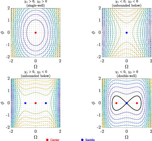
($\text { ● }$)At (0, 0): $\lambda^2 = -\chi_1$. Thus (0, 0) is a center if $\chi_1 \gt 0$ (single-well near the origin), and a saddle if $\chi_1 \lt 0$ (double-well with a local maximum at 0).

($\text { ● }$)At $\big(\pm\sqrt{\tfrac{-\chi_1}{\chi_2}},\,0\big)$ (when they exist): $\lambda^2 = 2\chi_1$. Hence these are centers if $\chi_1 \lt 0$ (minima of the double-well) and saddles if $\chi_1 \gt 0$.

Equivalently, $V^{^{\prime\prime}}(\Omega^*) = \chi_1+3\chi_2(\Omega^*)^2$: local minima of V correspond to centers and local maxima to saddles. The small-oscillation frequency satisfies $\omega_0 = \sqrt{V^{^{\prime\prime}}(\Omega^*)}$: in particular, $\omega_0 = \sqrt{\chi_1}$ at the origin when $\chi_1 \gt 0$, and $\omega_0 = \sqrt{-2\chi_1}$ about the off-origin centers when $\chi_1 \lt 0$ and $\chi_2 \gt 0$.

3.2. Energy landscape and phase-plane geometry

The quartic potential $V(\Omega)$ organizes the global geometry:

($\text { ● }$)Single-well ($\chi_1 \gt 0,\ \chi_2 \gt 0$): V has a unique minimum at $\Omega = 0$; level sets $\,\mathscr{H} = H \gt V(0)$ are closed, yielding families of periodic orbits surrounding the center (0, 0).

($\text { ● }$)Double-well ($\chi_1 \lt 0,\ \chi_2 \gt 0$): V has two minima at $\Omega = \pm\sqrt{\tfrac{-\chi_1}{\chi_2}}$ and a local maximum at $\Omega = 0$. The separatrix at the saddle energy $H = V(0)$ consists of a symmetric figure-eight made of two homoclinic orbits to the saddle (0, 0), enclosing periodic orbits around each minimum.

($\text { ● }$)Unbounded below ($\chi_2 \lt 0$): $V(\Omega)\to-\infty$ as $|\Omega|\to\infty$; accordingly, large-energy level sets are noncompact and trajectories can run away to infinity in finite evolution time η (since $\int^{\infty}\! \mathrm{d}\Omega/\sqrt{-\chi_2 \Omega^4}$ converges).

The period of finite-amplitude oscillations is amplitude-dependent and can be expressed via elliptic integrals by integrating $\Omega^{^{\prime}\,2} = 2\big(H-V(\Omega)\big)$; for $\chi_2 \gt 0$ (hardening) the frequency increases with amplitude (the period decreases), whereas for $\chi_2 \lt 0$ (softening) the opposite trend holds.
In the presence of weak damping and periodic forcing, the conserved energy picture breaks down and the phase portrait thickens into invariant tori, resonant islands, and chaotic layers. As the forcing amplitude or detuning increases, the system can undergo transitions from periodic to quasi-periodic and chaotic motions [8, 34]. For sufficiently small perturbations, most invariant tori persist by KAM theory; near low-order resonances, islands and separatrix layers appear. A Melnikov analysis (or numerical Poincaré sections) can diagnose transverse separatrix intersections, a classical route to Smale-horseshoe chaos in forced Duffing-type oscillators [36, 37].
In the phase portrait, closed orbits correspond to periodic wavetrains (recurrent envelope modulation), whereas homoclinic and heteroclinic connections represent localized pulses and kink or front transitions, respectively. The separatrix delineates bounded coherent packet dynamics from trajectories associated with large-amplitude excursions, which physically indicates a transition from sustained envelope coherence to strong modulation where the envelope approximation may approach its validity limits. The location of fixed points identifies equilibrium packet states, and their type (center or saddle) governs whether small perturbations lead to persistent oscillations or growth away from the coherent state.

4. Stochastic soliton solutions

System (20) is Hamiltonian. Multiplying the second equation in (20) by $\phi = \Omega^{^{\prime}}$ and integrating once gives the first integral
$\frac{1}{2} \phi^{2}+\frac{1}{2} \chi_{1} \Omega^{2}+\frac{1}{4} \chi_{2} \Omega^{4}=H$
where $H\in\mathbb{R}$ is the conserved energy. Eliminating $\phi$ yields the separable equation
$\left(\frac{\mathrm{d} \Omega}{\mathrm{~d} \eta}\right)^{2}=2 H-\chi_{1} \Omega^{2}-\frac{\chi_{2}}{2} \Omega^{4} .$
Hence,
$\pm\left(\eta-\eta_{0}\right)=\int \frac{\mathrm{d} \Omega}{\sqrt{2 H-\chi_{1} \Omega^{2}-\frac{\chi_{2}}{2} \Omega^{4}}}$
with a shift $\eta_{0}\in\mathbb{R}$. Because the radicand is quartic in Ω, explicit profiles are naturally expressed by Jacobi elliptic functions; solitary limits appear when a pair of turning points coalesce.
Introduce
$\Delta=\sqrt{\chi_{1}^{2}+4 \chi_{2} H}$
so that factorization of the quartic in (23) gives four (squared) turning levels
$\left\{\begin{array}{ll} \Omega_{r_{1}}^{2}=\frac{-\chi_{1}+\Delta}{\chi_{2}}, & \Omega_{r_{2}}^{2}=\frac{\chi_{1}+\Delta}{\chi_{2}} \\ \Omega_{r_{3}}^{2}=\frac{-\chi_{1}-\Delta}{\chi_{2}}, & \Omega_{r_{4}}^{2}=\frac{\chi_{1}-\Delta}{\chi_{2}} . \end{array}\right.$
Two energy thresholds will be used repeatedly:
$\begin{align*} H_{0} = 0, \qquad H_{1} = -\frac{\chi_{1}^{2}}{4\chi_{2}}.\end{align*}$
They separate homoclinic/heteroclinic dynamics from periodic (librational/rotational) motions in the $(\Omega,\phi)$ phase plane.
Case-1: $\chi_{1} \gt 0,\ \chi_{2} \gt 0$ ($H \gt H_{0},\ 0 \lt \Omega \lt \Omega_{r_1}$)
The effective potential has a single well at $\Omega = 0$ and energies H > 0 produce bounded oscillations. The envelope is
$\begin{align} \Omega\left(\eta\right)& = \pm \Omega_{r_1}\, \operatorname{cn}\!\left(\sqrt{\tfrac{\chi_{2}}{2}\,\left(\Omega_{r_1}^{2}+\Omega_{r_2}^{2}\right)}\,\left(\eta-\eta_{0}\right)\ \Big|\ m_{1}\right), \nonumber\\ m_{1} & = \frac{\Omega_{r_1}^{2}}{\Omega_{r_1}^{2}+\Omega_{r_2}^{2}}.\end{align}$
The associated stochastic solution is
$\begin{align} u\left(x,t\right) & = \pm \Omega_{r_1}\, \operatorname{cn}\!\left(\sqrt{\tfrac{\chi_{2}}{2}\,\left(\Omega_{r_1}^{2}+\Omega_{r_2}^{2}\right)}\,\left(x-vt-\eta_{0}\right)\ \Big|\ m_{1}\right)\,\nonumber\\ &\quad \times \mathrm{e}^{\,\mathrm{i}\left(-\kappa x+\omega t-\sigma W\left(t\right)\right)}.\end{align}$
In the limiting configuration $\Omega_{r_2}\to 0$ (i.e. $m_{1}\to 1^{-}$) the cn-wave degenerates to a localized pulse
$\Omega(\eta)= \pm \Omega_{r_{1}} \operatorname{sech}\left(\sqrt{\frac{\chi_{2}}{2}} \Omega_{r_{1}}\left(\eta-\eta_{0}\right)\right) .$
The corresponding stochastic solution is
$\begin{align} u\left(x,t\right) = \pm \Omega_{r_1}\,\mathrm{sech}\!\left(\sqrt{\tfrac{\chi_{2}}{2}}\,\Omega_{r_1}\left(x-vt-\eta_{0}\right)\right)\, \mathrm{e}^{\,\mathrm{i}\left(-\kappa x+\omega t-\sigma W\left(t\right)\right)}.\end{align}$
Case-2: $\chi_{1} \lt 0,\ \chi_{2} \lt 0$ ($H \lt H_{0},\ \Omega \gt \Omega_{r_1}$)
When both coefficients are negative and H < 0, the trajectories are unbounded beyond $\Omega_{r_1}$ and the profile takes the nc-form
$\begin{align} \Omega\left(\eta\right) &= \pm \Omega_{r_1}\, nc\!\left(\sqrt{-\tfrac{\chi_{2}}{2}\,\left(\Omega_{r_1}^{2}+\Omega_{r_2}^{2}\right)}\,\left(\eta-\eta_{0}\right)\ \Big|\ m_{2}\right),\nonumber\\ m_{2} & = \frac{\Omega_{r_2}^{2}}{\Omega_{r_1}^{2}+\Omega_{r_2}^{2}}.\end{align}$
The associated stochastic solution is
$\begin{align} u\left(x,t\right) & = \pm \Omega_{r_1}\, nc\!\left(\sqrt{-\tfrac{\chi_{2}}{2}\,\left(\Omega_{r_1}^{2}+\Omega_{r_2}^{2}\right)}\,\left(x-vt-\eta_{0}\right)\ \Big|\ m_{2}\right)\,\nonumber\\ &\quad \times \mathrm{e}^{\,\mathrm{i}\left(-\kappa x+\omega t-\sigma W\left(t\right)\right)}.\end{align}$
Case-3: $\chi_{1} \lt 0,\ \chi_{2} \gt 0$ (bright branch)
i

((i))$H_{1} \lt H \lt H_{0},\ \Omega_{r_2} = 0,\ \Omega_{r_1} = \sqrt{-\tfrac{2\chi_{1}}{\chi_{2}}}$.

At H = 0 one obtains the homoclinic orbit to the origin, i.e. the bright solitary wave

$\begin{align} \Omega\left(\eta\right) = \pm\sqrt{-\frac{2\chi_{1}}{\chi_{2}}}\; \mathrm{sech}\!\left(\sqrt{-\chi_{1}}\,\left(\eta-\eta_{0}\right)\right).\end{align}$
The corresponding stochastic solution is
$\begin{align} u\left(x,t\right) & = \pm\sqrt{-\frac{2\chi_{1}}{\chi_{2}}}\; \mathrm{sech}\!\left(\sqrt{-\chi_{1}}\,\left(x-vt-\eta_{0}\right)\right)\,\nonumber\\ &\quad \times \mathrm{e}^{\,\mathrm{i}\left(-\kappa x+\omega t-\sigma W\left(t\right)\right)}.\end{align}$

ii

((ii))$H_{1} \lt H \lt H_{0},\ \Omega_{r_3} \lt \Omega \lt \Omega_{r_1}$.

Away from the homoclinic level the periodic bright train is given by

$\begin{align} \Omega\left(\eta\right) &= \pm \Omega_{r_1}\, dn\!\left(\Omega_{r_1}\sqrt{\tfrac{\chi_{2}}{2}}\,\left(\eta-\eta_{0}\right)\ \Big|\ m_{3}\right),\nonumber\\ m_{3} &= \frac{\Omega_{r_1}^{2}-\Omega_{r_3}^{2}}{\Omega_{r_1}^{2}}.\end{align}$
The corresponding stochastic solution is
$\begin{align} u\left(x,t\right) &= \pm \Omega_{r_1}\, dn\!\left(\Omega_{r_1}\sqrt{\tfrac{\chi_{2}}{2}}\,\left(x-vt-\eta_{0}\right)\ \Big|\ m_{3}\right)\,\nonumber\\ &\quad \times \mathrm{e}^{\,\mathrm{i}\left(-\kappa x+\omega t-\sigma W\left(t\right)\right)}.\end{align}$

Case-4: $\chi_{1} \gt 0,\ \chi_{2} \lt 0$ (dark/kink branch)
i

((i))$H_{0} \lt H \lt H_{1},\ \Omega_{r_1} = \Omega_{r_3} = -\chi_{1}/\chi_{2}$.

At the double root the heteroclinic connection yields the dark (kink) profile

$\begin{align} \Omega\left(\eta\right) = \pm\sqrt{-\frac{\chi_{1}}{\chi_{2}}}\; \tanh\!\left(\sqrt{\tfrac{\chi_{1}}{2}}\,\left(\eta-\eta_{0}\right)\right).\end{align}$
The corresponding stochastic solution is
$\begin{align} u\left(x,t\right) & = \pm\sqrt{-\frac{\chi_{1}}{\chi_{2}}}\; \tanh\!\left(\sqrt{\tfrac{\chi_{1}}{2}}\,\left(x-vt-\eta_{0}\right)\right)\,\nonumber\\ &\quad \times \mathrm{e}^{\,\mathrm{i}\left(-\kappa x+\omega t-\sigma W\left(t\right)\right)}.\end{align}$

ii

((ii))$H_{0} \lt H \lt H_{1},\ 0 \lt \Omega \lt \Omega_{r_3} \lt \Omega_{r_1}$.

The associated periodic front-like modulation is

$\begin{align} \Omega\left(\eta\right)& = \pm \Omega_{r_3}\, cd\!\left(\sqrt{-\tfrac{\chi_{2}}{2}}\,\Omega_{r_1}\,\left(\eta-\eta_{0}\right)\ \Big|\ m_{4}\right),\nonumber\\ m_{4}& = \left(\frac{\Omega_{r_3}}{\Omega_{r_1}}\right)^{2}.\end{align}$
The corresponding stochastic solution is
$\begin{align} u\left(x,t\right)& = \pm \Omega_{r_3}\, cd\!\left(\sqrt{-\tfrac{\chi_{2}}{2}}\,\Omega_{r_1}\,\left(x-vt-\eta_{0}\right)\ \Big|\ m_{4}\right)\,\nonumber\\ &\quad \times \mathrm{e}^{\,\mathrm{i}\left(-\kappa x+\omega t-\sigma W\left(t\right)\right)}.\end{align}$

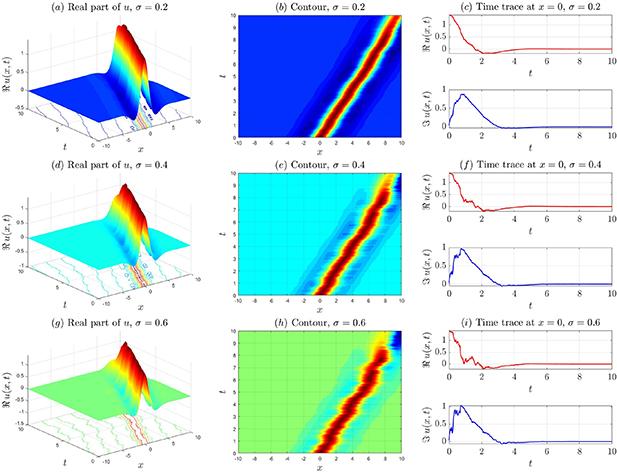
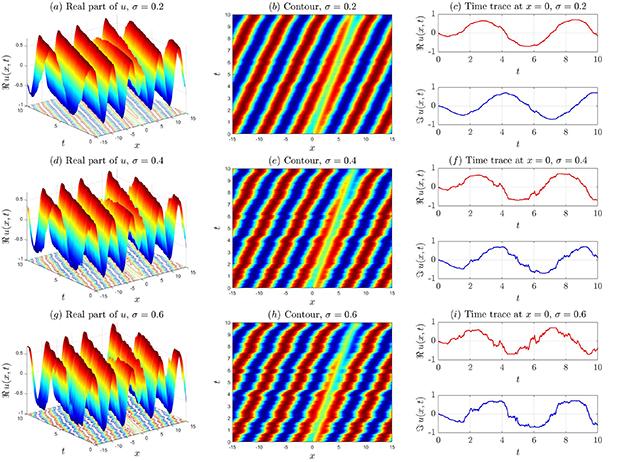
In the present model the stochasticity enters as multiplicative Stratonovich phase noise, so the random gauge representation implies that increasing σ primarily enhances phase diffusion rather than directly deforming the envelope modulus. Consequently, as σ increases, the real and imaginary parts exhibit stronger apparent fluctuations (phase wandering), while the amplitude $|q(x,t)|$ remains essentially unchanged for the same deterministic envelope parameters. To make this effect visible without entering a regime where the phase becomes fully decorrelated, we select representative weak, moderate, and strong noise levels $\sigma\in\{0.2,0.4,0.6\}$ (dimensionless), corresponding to increasing values of the effective phase-variance scale $\sigma^{2}T$ over the plotted time horizon T. This yields a clear, monotone trend in phase coherence while keeping the underlying envelope dynamics comparable across panels.
Representative profiles and noise-intensity effects for the bright and dark/kink branches are displayed in figure 1-5.
Figure 1. Phase analysis of bifurcation in dynamical system (20).
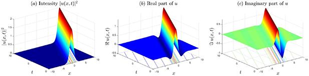
Figure 2. Representative coherent-wave solution (32) of the NBWP model for the parameter set $\chi_1 = -1$, χ2 = 1, a = 1, β = 0.6, δ = 0, κ = 1, v = 1, $\omega$ = 1. Panels show (a) amplitude $|u(x,t)|$, (b) $\Re(u(x,t))$, and (c) $\Im(u(x,t))$ at t = 1. For this parameter regime the solution corresponds to a bright solitary wave.
Figure 3. Effect of phase-noise intensity on the solution (32), using identical deterministic envelope parameters and varying $\sigma\in\{0.2,0.4,0.6\}$. As σ increases, phase diffusion becomes stronger, producing increased fluctuations in $\Re(u)$ and $\Im(u)$ (apparent profile wandering), while the modulus $|u|$ remains essentially unchanged because the noise acts through a multiplicative random phase factor in the Stratonovich sense.
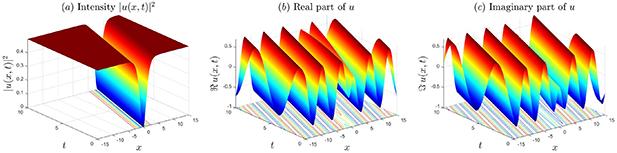
Figure 4. Second representative solution branch (35) for the parameter set χ1 = 1, $\chi_2 = -2$, a = 1, β = 0.6, δ = 0, κ = 1, v = 0.8, $\omega$ = 1. Panels show (a) amplitude $|u(x,t)|$, (b) $\Re(u(x,t))$, and (c) $\Im(u(x,t))$ at t = 1.0. This parameter regime corresponds to a dark/kink-type wave.
Figure 5. Noise-intensity comparison for the solution (35) with $\sigma\in\{0.2,0.4,0.6\}$. Increasing σ primarily enhances phase wandering, which is reflected in the oscillatory structure of $\Re(u)$ and $\Im(u)$, while the envelope modulus $|u|$ remains essentially unchanged for fixed deterministic parameters.
Remarks. (i) The solitary limits (32) and (36) arise as the elliptic modulus tends to 1, recovering the homoclinic (bright) and heteroclinic (dark) phase-plane orbits. (ii) The sign pairs $(\chi_{1},\chi_{2})$ listed above are the only ones that produce finite-energy localized waves; the remaining sign combinations generate either small-amplitude linear oscillations about the origin or unbounded trajectories.

5. Quasi-periodic to chaotic dynamics

To study the chaotic analysis within the above system, we will introduce an external force in the form of a periodic force to perturb the system. It yields the following autonomous dynamical system:
$\begin{equation} \begin{cases} \frac{\mathrm{d} \Omega}{\mathrm{d}\eta} = \phi,\\ \frac{\mathrm{d} \phi}{\mathrm{d} \eta} = -\chi_1\Omega-\chi_2\Omega^3+q_0 \mathcal{F}\left(\eta\right), \end{cases}\end{equation}$
where $\mathcal{F}(\eta)$ is the external applied force to cause some disturbance in the periodic motion of the dynamical system (20) represents the strength and frequency of the external force. In this work, we introduce three types of applied force such as: trigonometric function, hyperbolic, and Gaussian functions. This system captures the underlying dynamics and acts as a strong candidate for exploring chaotic behavior.

5.1. Melnikov method for chaos

We now justify the onset of chaotic dynamics under weak time-periodic forcing using the Melnikov approach [22, 23].
For $\chi_1 \lt 0$, $\chi_2 \gt 0$ there exists a homoclinic (bright) orbit connecting the saddle at the origin:
$\begin{align} \Omega_h\left(\eta\right)& = \pm A_h\,\mathrm{sech}\left(\kappa\left(\eta-\eta_0\right)\right),\nonumber\\ \phi_h\left(\eta\right) &= \Omega_h^{^{\prime}}\left(\eta\right) = \mp A_h\,\kappa\,\mathrm{sech}\left(\kappa\left(\eta-\eta_0\right)\right)\tanh\left(\kappa\left(\eta-\eta_0\right)\right),\end{align}$
with $A_h = \sqrt{-\,2\chi_1/\chi_2}$ and $\kappa = \sqrt{-\,\chi_1}$.
Introduce a small time-dependent perturbation (forcing in (40)):
$\begin{align} \frac{\mathrm{d}\Omega}{\mathrm{d}\eta} &= \phi,\quad \frac{\mathrm{d}\phi}{\mathrm{d}\eta} = -\chi_1\Omega-\chi_2\Omega^3 \;+\; \varepsilon\,q_0\,\mathcal{F}\left(\eta\right),\nonumber\\ &\quad 0 \lt \varepsilon\ll1 ,\end{align}$
so that the invariant manifolds of the saddle may split. The Melnikov function,
$\begin{align} M\left(\eta_0\right) &= \int_{-\infty}^{\infty}\nabla \mathscr{H}\left(\Omega_h,\phi_h\right)\cdot \begin{bmatrix}0\\ q_0\,\mathcal{F}\left(\eta+\eta_0\right)\end{bmatrix}\,\mathrm{d}\eta\nonumber\\ & = \;q_0\int_{-\infty}^{\infty}\phi_h\left(\eta\right)\,\mathcal{F}\left(\eta+\eta_0\right)\,\mathrm{d}\eta ,\end{align}$
measures the signed distance between the stable and unstable manifolds on a Poincaré section. Simple zeros of $M(\eta_0)$ imply a transverse homoclinic intersection and the presence of a Smale horseshoe (hence chaotic dynamics).
The Melnikov calculation carried out below is formulated for a deterministically and periodically forced Hamiltonian traveling-wave system. This is intentional: in our stochastic NBWP model the Stratonovich multiplicative phase noise is removed from the amplitude equation by a random gauge transformation, so the reduced oscillator governing the traveling-wave envelope modulus is deterministic. The periodic forcing term represents an external deterministic perturbation (for example, idealized tidal or topographic modulation, or parametric excitation) acting on the reduced dynamics. Therefore, the Melnikov function provides a parameter-dependent criterion for transverse intersection of the stable and unstable manifolds of the unperturbed homoclinic orbit and hence a threshold for the onset of chaotic modulation in the forced deterministic reduced system.
(i) Trigonometric forcing $\mathcal{F}(\eta) = \cos(\omega\eta)$. Using that $\phi$h is odd and integrating by parts (with $\text{sech}^{^{\prime}} = -\,\text{sech}\tanh$), one obtains a closed form:
$\begin{align} M\left(\eta_0\right) & = q_0\int_{-\infty}^{\infty}\phi_h\left(\eta\right)\cos\left(\omega\left(\eta+\eta_0\right)\right)\,\mathrm{d}\eta = -\,\varepsilon\,q_0\,\mathcal{A}\left(\omega\right)\,\sin\left(\omega \eta_0\right),\end{align}$
$\begin{align} \mathcal{A}\left(\omega\right) & = A_h\frac{\omega}{\kappa}\,\pi\ \text{sech}\!\left(\frac{\pi\omega}{2\kappa}\right),\quad A_h = \sqrt{-\frac{2\chi_1}{\chi_2}},\ \ \kappa = \sqrt{-\chi_1}.\end{align}$
Thus M has simple zeros at $\eta_0 = \tfrac{n\pi}{\omega}$ ($n\in\mathbb{Z}$) whenever $\omega$ ≠ 0 and $q_0\neq0$, guaranteeing a transverse manifold intersection. The amplitude $\mathcal{A}(\omega)$ controls the splitting size; it decays monotonically for large $\omega$ and is maximal at $\omega\approx0^+$.
(ii) Localized (Gaussian) forcing $\mathcal{F}(\eta) = \exp$$\big(-\tfrac{1}{2}(\omega\eta)^2\big)$. In this case
$\begin{align} M\left(\eta_0\right) & = q_0\int_{-\infty}^{\infty}\phi_h\left(\eta\right)\, \exp\!\left(-\frac{\omega^2}{2}\left(\eta+\eta_0\right)^2\right)\,\mathrm{d}\eta \nonumber\\ & = \;q_0\,\left(\phi_h * G_\omega\right)\left(-\,\eta_0\right),\end{align}$
with $G_\omega(\eta) = \mathrm{e}^{-(\omega\eta)^2/2}$ even and $*$ denoting convolution. Since $\phi$h is odd, $M(\eta_0)$ is an odd function with $M(0) = 0$. Moreover,
$equation*$
so the zero at η0 = 0 is simple for every $\omega$ > 0 and $q_0\neq0$. Hence the stable/unstable manifolds intersect transversely and chaotic dynamics ensue.
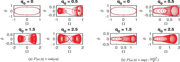
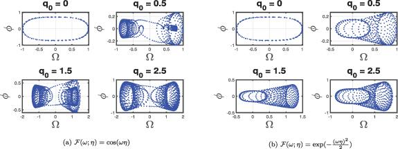
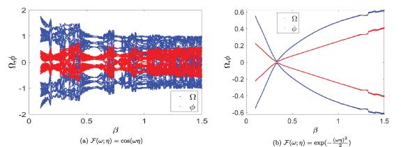
Consequences. For either forcing, the existence of simple zeros of M implies a horseshoe dynamics near the former homoclinic loop, consistent with the numerics: scattered Poincaré sections, positive Lyapunov exponents, and cascades in the bifurcation diagrams (cf figures 6-10). The Melnikov amplitude $\mathcal{A}(\omega)$ explains the observed dependence on the forcing frequency: low frequencies yield wider manifold splitting and more prominent chaotic layers; high frequencies suppress the splitting exponentially through the $\text{sech}(\cdot)$ factor in (45).
Figure 6. The equilibrium point labeled C denotes a center (linearly neutrally stable equilibrium) associated with small-amplitude periodic wavetrains, while S denotes a saddle equilibrium whose stable/unstable manifolds organize separatrices. Homoclinic orbits to S correspond to localized solitary pulses, and heteroclinic connections (when present) correspond to kink/front-type transitions. Phase portrait illustration of system (40) using parameters $ \chi_1 = 0.1,\chi_2 = 0.8,q_0 = 0.03 $ and initial conditions $ \Omega(0) $ = 1, $ \phi(0) = 0 $ with two perturbations $\mathcal{F} (\omega;\eta):\,$(a) $~~\cos(\omega\eta)$ and (b) $~~ \exp(- \frac{(\omega \eta)^2}{2})$.
Figure 7. Poincare illustration of system (40) using parameters $ \chi_1 = 0.1,\chi_2 = 0.8,q_0 = 0.03 $ and initial conditions $ \Omega(0) $ = 1, $ \phi(0) = 0 $ with two perturbations $\mathcal{F} (\omega;\eta):\,$(a) $\cos(\omega\eta)$ and (b) $\exp(- \frac{(\omega \eta)^2}{2})$.
Figure 8. The abscissa is the control parameter (e.g. forcing amplitude ϵ, forcing frequency Ω, detuning parameter, or wave speed v), and the ordinate is the sampled envelope observable (e.g. peak amplitude $\max_\xi g(\xi)$ or Poincaré-section value of g). Single branches indicate periodic responses; branch splitting and dense point sets indicate quasi-periodic or chaotic modulation. Bifurcation diagram illustration of system (40) using parameters $ \chi_1 = 0.15,q_0 = 0.5, \omega = 0.1$ and initial conditions $ \Omega(0) $ = 1, $ \phi(0) = 0 $ with two perturbations $\mathcal{F} (\omega;\eta):\,$(a) $~~\cos(\omega\eta)$ and (b) $\exp(- \frac{(\omega \eta)^2}{2})$.
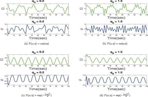
Figure 9. Time series of $\langle\mathcal{O}(t)\rangle$ versus time t for the forced reduced dynamics, where $\mathcal{O}(t) = \langle\cdot\rangle$ is the plotted observable (e.g. $|u|$, or peak amplitude). The ordinate is reported in $\langle\text{dimensionless units/physical units}\rangle$ consistent with the non-dimensionalization used in equation (1). Time series illustration of system (40) using parameters $ \chi_1 = 0.1,\chi_2 = 0.8,q_0 = 0.3 $ and initial conditions $ \Omega(0) $ = 1, $ \phi(0) = 0 $ with two perturbations $\mathcal{F} (\omega;\eta):\,$(a), (b) $\cos(\omega\eta)$ and (c), (d) $\exp(- \frac{(\omega \eta)^2}{2})$.
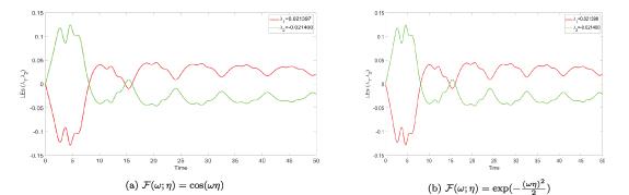
Figure 10. Lyapunov exponent illustration of system (40) using parameters $ \chi_1 = 0.1,\chi_2 = 0.5,q_0 = 0.2, \omega = 0.3 $ and initial conditions $ \Omega(0) $ = $ \phi(0) = 0 $ with two perturbations $\mathcal{F} (\omega;\eta):$ (a) $\cos(\omega\eta)$ and (b) $\exp(- \frac{(\omega \eta)^2}{2})$.
Remark. The analysis above uses the bright homoclinic orbit (41) (case $\chi_1 \lt 0,\ \chi_2 \gt 0$). An analogous construction applies when the reduced phase portrait admits a heteroclinic (dark/kink) connection (case $\chi_1 \gt 0,\ \chi_2 \lt 0$); the Melnikov integral keeps the form (43) with $(\Omega_h,\phi_h)$ replaced by the corresponding kink profile.
The (maximal) Lyapunov exponent $\lambda_{\max}$ measures the mean exponential rate at which two nearby trajectories in the phase space separate, i.e. $\|\delta \mathbf{X}(t)\|\sim \|\delta \mathbf{X}(0)\|\mathrm{e}^{\lambda_{\max} t}$. Hence, $\lambda_{\max} \gt 0$ is the standard quantitative signature of chaos and implies strong sensitivity to initial conditions (practical loss of predictability of the envelope dynamics), whereas $\lambda_{\max} = 0$ typically corresponds to quasi-periodic motion and $\lambda_{\max} \lt 0$ indicates convergence to a stable periodic orbit or equilibrium. In the present context, a positive $\lambda_{\max}$ means that small uncertainties in the initial wavepacket or weak environmental variability can rapidly amplify, leading to irregular modulation and run-to-run variability in packet amplitude and localization.
We emphasize that a stochastic Melnikov theory would be required if amplitude or mixed noise terms were introduced into the reduced dynamics; such genuinely stochastic perturbations are beyond the scope of the present work and are left for future investigation.
We emphasize that equation (1) accounts only for Stratonovich multiplicative phase noise; stochastic forcing in the amplitude or coupled amplitude and phase channels (which may arise from unresolved turbulence, variable dissipation, or random stratification and topography) is not considered here. Such extensions can be modeled, for example, by adding terms of the form $\sigma_a u\circ \mathrm{d}W_t$ (amplitude noise) or more general state-dependent diffusion coefficients $\Sigma(u)\circ \mathrm{d}W_t$. In these cases the exact random gauge elimination generally breaks down, and the spectral stability and long-time dynamics become genuinely stochastic (requiring, for example, moment equations, stochastic averaging, or sample-path numerics). Investigating how amplitude and mixed noise modifies MI thresholds and the onset of irregular modulation is an important direction for future work.

6. Conclusion

This work developed a stochastic extension of the non Boussinesq wavepacket model as an NLS type envelope description for internal waves in strongly stratified media. Multiplicative Stratonovich noise was introduced in the phase to represent realistic environmental fluctuations. A gauge based reduction produced a deterministic Hamiltonian envelope system that preserves the essential balance between dispersion and nonlinearity and organizes periodic states localized envelopes and front like transitions.
The main contributions of this work can be summarized as follows. We formulate a stochastic NBWP model by incorporating Stratonovich multiplicative phase noise, and we show that this choice admits a gauge transformation that removes the explicit noise from the envelope dynamics, yielding a tractable deterministic reduction. Using a traveling-wave reduction, we derive a deterministic Hamiltonian envelope system and classify its coherent structures (periodic wavetrains, localized pulses, and kink and front profiles) within a single phase-plane framework. We provide an explicit MI characterization in terms of effective dispersion and cubic nonlinearity, and we clarify the distinct roles of higher-order dispersion, which produces band shifting, versus phase noise, which does not change the leading MI gain. Finally, we connect the reduced Hamiltonian dynamics to routes to chaos under weak periodic forcing by combining a Melnikov criterion with numerical diagnostics (Poincaré sections, bifurcation diagrams, and Lyapunov exponents), thereby offering a unified stability to complexity pipeline for NBWP type systems.
The present results have direct relevance to internal-wave dynamics in strongly stratified environments. First, the traveling-wave phase-plane classification identifies parameter regimes supporting localized pulses and kink/front profiles, which can be interpreted as robust packet-like transport events or sharp transition layers in stratified channels and pycnoclines. Second, the MI conditions provide an operational criterion for the onset of sideband growth, offering a mechanism-based indicator of when an initially coherent wavepacket may evolve toward envelope breakup, enhanced shear, and elevated mixing potential. Third, the forced-dynamics analysis (Melnikov threshold together with Poincaré sections and Lyapunov exponents) supplies a quantitative predictor for transitions from regular packet evolution to irregular (chaotic) modulation under weak external perturbations, a scenario consistent with tidal forcing, topographic interactions, or slowly varying background stratification. Collectively, these diagnostics link model parameters to observable outcomes (coherence persistence, instability-driven breakup, and loss of predictability), which is useful for interpreting laboratory and field measurements within the validity range of the envelope approximation.
Finally, although the Stratonovich phase noise can be removed from the evolution equation by a random gauge, the physical field remains stochastic through the inverse transformation, so the model retains a clear interpretation in terms of realization-dependent wavepacket phases.
The MI analysis identified the conditions that govern sideband amplification and clarified how higher order dispersion shifts the unstable band while phase noise does not alter the leading growth rate. Under weak periodic forcing the system exhibits a transition from regular oscillations to chaotic motion. Melnikov arguments and numerical diagnostics including sections bifurcation diagrams and Lyapunov exponents confirmed transverse manifold intersections and the emergence of complex dynamics.
Together these results offer a unified analytical and computational framework for stability coherence and transition to chaos in non Boussinesq media. The approach can be adapted to spatially varying parameters broadband fluctuations and higher dimensional settings to support predictive studies of internal wave packets in geophysical applications.
Finally, while the Stratonovich phase noise does not alter the closed-form envelope modulus of the Jacobi elliptic and solitary profiles, it produces realization-dependent phase modulation that is relevant to phase-sensitive observables and provides a clean separation between deterministic amplitude dynamics and stochastic coherence effects.
1
DosserH V, SutherlandB R2011Weakly nonlinear non-Boussinesq internal gravity wavepacketsPhysica d240 346356

DOI

2
ClarkH A, SutherlandB R2009Schlieren measurements of internal waves in non-Boussinesq fluidsExp. Fluids47 183193

DOI

3
WangH, ChenL, LiuH2015Nonlinear dynamics and exact travelling wave solutions in the non-Boussinesq wavepacket model2015 12th Int. Conf. on Fuzzy Systems and Knowledge Discovery (FSKD) IEEE 25392543

DOI

4
CraikA D1988Wave Interactions and Fluid Flows Cambridge University Press

5
Van den BremerT S, SutherlandB R2014The mean flow and long waves induced by two-dimensional internal gravity wavepacketsPhys. Fluids26 106601

DOI

6
RafiqM H, RafiqM N, AlsaudH2025Chaotic dynamics and exact solutions for $(3+1)$-dimensional KdV-Calogero-Bogoyavlenskii-Schiff modelPhys. Lett. A20 130751

DOI

7
ArnousA H2025Lie symmetries, stability and chaotic dynamics of solitons in nematic liquid crystals with stochastic perturbationChaos Solitons Fractals199 116730

DOI

8
RafiqM N, RafiqM H, AlsaudH2025New insights into the diversity of stochastic solutions and dynamical analysis for the complex cubic NLSE with δ-potential through Brownian processCommun. Theor. Phys.77 075001

DOI

9
De SzoekeR A, SamelsonR M2002The duality between the Boussinesq and non-Boussinesq hydrostatic equations of motionJ. Phys. Oceanogr.32 21942303

DOI

10
AiJ, LawA W, YuS2006On Boussinesq and non-Boussinesq starting forced plumesJ. Fluid Mech.558 357386

DOI

11
SongY T, HouT Y2006Parametric vertical coordinate formulation for multiscale, Boussinesq and non-Boussinesq ocean modelingOcean Modelling11 298332

DOI

12
BoisP A2007Joseph Boussinesq (1842-1929): a pioneer of mechanical modelling at the end of the 19th centuryC. R. Mec.335 479495

DOI

13
SzewcK, PozorskiJ, TaniereA2011Modeling of natural convection with smoothed particle hydrodynamics: non-Boussinesq formulationInt. J. Heat Mass Transfer54 48074816

DOI

14
GreatbatchR J, LuY, CaiY2001Relaxing the Boussinesq approximation in ocean circulation modelsJ. Atmos. Ocean. Technol.18 19111923

DOI

15
BordenZ, KoblitzT, MeiburgE2012Turbulent mixing and wave radiation in non-Boussinesq internal boresPhys. Fluids24 082106

DOI

16
ZhangY, CaoY2018A numerical study on the non-Boussinesq effect in the natural convection in horizontal annulusPhys. Fluids30 040902

DOI

17
AgrawalR, BoseS, MoinP2022Wall modeled LES of the Boeing speed bump using a non-Boussinesq modeling frameworkCenter for Turbulence Research Annual Research Briefs 2022pp 4358 https://web.stanford.edu/group/ctr/ResBriefs/2022/06_Agrawal.pdf

18
ArnousA H2025Chaotic dynamics and bifurcation analysis of optical solitons in birefringent fibers governed by the Sasa-Satsuma equation with stochastic perturbationNonlinear Dyn.113 1846918484

DOI

19
WangDet al2025Launching by cavitationScience389 9351009

DOI

20
MouD S, SiZ Z, QiuW X, DaiC Q2025Optical soliton formation and dynamic characteristics in photonic Moiré latticesOpt. Laser Technol.181 111774

DOI

21
XuT Z, LiuJ H, DaiC Q, WangX Y2025Multipole solitons of fractional second-third order nonlinear Schrödinger system with PT symmetric potentialNonlinear Dyn.113 3271332722

DOI

22
ZhouY, ZhaoP, GuoY2025Melnikov analysis of chaotic dynamics in an impact oscillator systemInt. J. Non-Linear Mech.171 105027

DOI

23
NiuJ, LiuR, ShenY, YangS2019Chaos detection of Duffing system with fractional-order derivative by Melnikov methodChaos29 123106

DOI

24
RazaN, GandariasM L, RafiqM H, RanaZ, MuhammadT2025A deep analytical investigation of solitons and nonlinear dynamics in the (3+1)-dimensional hirota-type equationNonlinear Dyn.113 2802328037

DOI

25
TélT, GruizM2006Chaotic Dynamics: An Introduction Based on Classical Mechanics Cambridge University Press

26
YounasU, HussainE, MuhammadJ, GarayevM, El-MeligyM2025Bifurcation analysis, chaotic behavior, sensitivity demonstration and dynamics of fractional solitary waves to nonlinear dynamical systemAin Shams Eng. J.16 103242

DOI

27
AkramS, ur RahmanM, AL-EssaL A2025A comprehensive dynamical analysis of $(2+ 1)$-dimensional nonlinear electrical transmission line model with Atangana-Baleanu derivativePhys. Lett. A555 130762

DOI

28
KazmiS S, JhangeerA, RiazB M2026Data-driven approach to shallow water equation in ocean engineering: Multi-soliton solutions, chaos, and sensitivity analysisMath. Comput. Simul.241 573595

DOI

29
MadadiM, HosseiniK, AhmadS2026Oblique line rogue wave solutions of the generalized extended KP equation: from bilinear forms to KP hierarchyEur. Phys. J. Plus141 276

DOI

30
AfridiI M2025Stochastic dynamics of symmetry reductions to the parabolic nonlinear model in metamaterialsResults Eng.26 105630

DOI

31
WangH, TianS F, ChenY2019Characteristics of the breather waves, rogue waves and solitary waves in an extended $(3+1)$-dimensional Kadomtsev-Petviashvili equationInt. J. Numer. Methods Heat Fluid Flow29 29642976

DOI

32
AlazmanI, MishraM N, AlkahtaniB S, ur RahmanM2025Comparative study of novel solitary wave solutions with unveiling bifurcation and chaotic structure modelled by stochastic dynamical systemZ. Naturforsch. A80 285311

DOI

33
BiondiniG, FagerstromE2015The integrable nature of modulational instabilitySIAM J. Appl. Math.75 136163

DOI

34
özerA, AkinE2005Tools for detecting chaosSakarya Univ. J. Sci.9 6066

DOI

35
BelykhV N, BykovV V1998Bifurcations for heteroclinic orbits of a periodic motion and a saddle-focus and dynamical chaosChaos Solitons Fractals9 18

DOI

36
YagasakiK1996The Melnikov theory for subharmonics and their bifurcations in forced oscillationsSIAM J. Appl. Math.56 17201765

DOI

37
GideaM, de la LlaveR2018Global Melnikov theory in Hamiltonian systems with general time-dependent perturbationsJ. Nonlinear Sci.28 16572307

DOI

Outlines

/